Elsevier Editorial System(tm) for Applied Energy Manuscript Draft
Manuscript Number:
Title: Dynamic modeling of a PV pumping system with special consideration on water demand Article Type: Special Issue: ICAE2012
Keywords: renewable energy resources, solar energy, photovoltaic system, pumping system, water demand
Corresponding Author: Mr. Pietro Elia Campana, Corresponding Author's Institution:
First Author: Pietro Elia Campana
Order of Authors: Pietro Elia Campana; Hailong Li; Jinyue Yan
Abstract: The exploitation of solar energy in remote areas through photovoltaic (PV) systems is an attractive solution for water pumping for irrigation systems. The design of a photovoltaic water pumping system (PVWPS) strictly depends on the estimation of the crop water requirements and land use since the water demand varies during the watering season and the solar irradiation changes time by time. It is of significance to conduct dynamic simulations in order to achieve the successful and optimal design. The aim of this paper is to develop a dynamic modeling tool for the design of a of photovoltaic water pumping system by combining the models of the water demand, the solar PV power and the pumping system, which can be used to validate the design procedure in terms of matching between water demand and water supply. Both alternate current (AC) and direct current (DC) pumps and both fixed and two-axis tracking PV array were analyzed. The tool has been applied in a case study. Results show that it has the ability to do rapid design and optimization of PV water pumping system by reducing the power peak and selecting the proper devices from both technical and economic
viewpoints. Among the different alternatives considered in this study, the AC fixed system represented the best cost effective solution.
Referees
1. Han Song
PhD student
School of Sustainable Development of Society and Technology, Mälardalen University, SE-72123 Västerås, Sweden
song.han@mdh.se 2. Umberto Desideri
Professor
Department of Industrial Engineering, University of Perugia,
Via G. Duranti 93 -
06125 Perugia, Italy
umberto.desideri@unipg.it
3. Takeshita Takayuki
Project Lecturer The University of Tokyo takeshita@ir3s.u-tokyo.ac.jp
umberto.desideri@unipg.it
Highlights
1. Evaluation of water demand and solar energy is essential for PV pumping system. 2. The design for a PV water pumping system has been optimized based on dynamic
simulations
3. It is important to conduct dynamic simulations to check the matching between water demand and water supply.
4. AC pump driven by the fixed PV array is the most cost-effective solution.
DYNAMIC MODELING OF A PV PUMPING SYSTEM WITH SPECIAL CONSIDERATION ON WATER DEMAND
1Pietro Elia Campana1*, Hailong Li1, Jinyue Yan1, 2* 2
1
School of Sustainable Development of Society and Technology, Mälardalen University, SE-72123 Västerås, 3
Sweden 4
2
School of Chemical Science, Royal Institute of Technology, SE-144 Stockholm, Sweden 5
6
ABSTRACT
7
The exploitation of solar energy in remote areas through photovoltaic (PV) systems is an attractive solution for 8
water pumping for irrigation systems. The design of a photovoltaic water pumping system (PVWPS) strictly 9
depends on the estimation of the crop water requirements and land use since the water demand varies during 10
the watering season and the solar irradiation changes time by time. It is of significance to conduct dynamic 11
simulations in order to achieve the successful and optimal design. The aim of this paper is to develop a dynamic 12
modeling tool for the design of a of photovoltaic water pumping system by combining the models of the water 13
demand, the solar PV power and the pumping system, which can be used to validate the design procedure in 14
terms of matching between water demand and water supply. Both alternate current (AC) and direct current (DC) 15
pumps and both fixed and two-axis tracking PV array were analyzed. The tool has been applied in a case study. 16
Results show that it has the ability to do rapid design and optimization of PV water pumping system by reducing 17
the power peak and selecting the proper devices from both technical and economic viewpoints. Among the 18
different alternatives considered in this study, the AC fixed system represented the best cost effective solution. 19
20
Keywords: renewable energy resources, solar energy, photovoltaic system, pumping system, water demand.
21 22 23 24 25 26 27 28 29 30 31 *Manuscript
NOMENCLATURE 33 Abbreviation 34 AC Alternate current 35 DC Direct current 36
ICC Initial investment cost 37
MPPT Maximum power point tracker 38
PV Photovoltaic
39
PVWPS Photovoltaic water pumping system 40
SCS Soil conservation service 41
42
Symbols 43
ea Actual vapour pressure [kPa]
44
Eh Hydraulic energy [kWh/day]
45
es Saturation vapour pressure [kPa]
46
ET0 Reference evapotranspiration [mm/day]
47
ETc Evapotranspiration in cultural conditions [mm/day]
48
EX Extraterrestrial radiation (kWh/m2) 49
g Gravity acceleration [m/s2] 50
G Soil heat flux density [MJ/m2day] 51
GH Global horizontal radiation (kWh/m2) 52
H Total dynamic head [m] 53
Ib Beam radiation [Wh/m2]
54
Id Diffuse radiation [Wh/m2]
55
Itot Global radiation on the array [Wh/m2]
56
Itot,d Daily total radiation [kWh/m2/day]
57
Kb(θ) Incidence angle modifier
58
Kc Cultural coefficient
59
Kd Incidence modifier for diffuse radiation
60
LI Longwave incoming radiation (kWh/m2) 61
LO Longwave outgoing radiation (kWh/m2) 62
NOCT Nominal operating cell temperature [°C] 63 P Precipitation (mm) 64 P(T,θ) Power output [W] 65 Q Water flow [l/s] 66 RH Relative humidity (%) 67
Rn Net radiation at crop surface [MJ/m2day] 68 T Temperature [°C] 69 Ta Ambient temperature [°C] 70 Tc Cell temperature [°C] 71 Tr Reference temperature [°C] 72
u2 Wind speed at 2 m height [m/s]
73
Wg Water gross volume [mm/day]
74
WS Wind speed (m/s)
75
Wt Watered height [mm]
76
α Power temperature coefficient [%/°C] 77
γ Psychrometric constant [kPa/°C] 78
Δ Slope vapour pressure curve [kPa/°C] 79
η0b Optical efficiency for beam radiation [%]
80
ηs System efficiency [%]
81
ηp Pump efficiency [%]
82
ηPV,T PV module thermal efficiency [%]
83
ηw Electric wires efficiency[%]
84 Θ Angle of incidence [°] 85 ρ Water density [kg/m3] 86 1. INTRODUCTION 87
The availability of electricity in remote areas is one of the main issues regarding the design and operation of 88
irrigation systems. Nevertheless, it is quite common in the developing countries that the access to the electric grid 89
is unavailable. With the development of photovoltaic (PV) technology that can convert the solar energy to 90
electricity, using PV cells has become a more attractive solution to provide the required power for the water 91
pumping system, especially in the areas that have abundant solar energy resources [1]. The high technical 92
reliability of PVWPSs for irrigation purposes, their long term economic viability and recent developments as well 93
as the weaknesses have been shown by several studies and field experiences. The knowledge and the 94
competencies achieved in this field resulted as starting point and recommendations for further and future 95
programmes worldwide [2, 3]. For example, in 2009 the Government of Bangladesh has set as target for 2014 to 96
install more than 10000 PVWPS for irrigation with a total installed capacity of 10 MWp. Only in 2010 India has
97
installed more than 50 MWp PV off-grid systems of which pumping system represent a large part [4].
98
Many studies have been carried out in the development of the PVWPS focusing on the system sizing, system 99
modeling, economic performance and environmental feasibility. Models have been presented for the estimation 100
generator, pumping system power consumption and instantaneous water flow output have been conducted [11]. 103
Based on the available models, the approaches regarding the system optimization have been developed [12]. In 104
addition, economic and environmental evaluations showed the feasibility of photovoltaic pumping system 105
compared to traditional systems driven by diesel engines [13]. 106
The main R&D gaps for the implementation of the PVWPSs exist not only in the technologies of PV and pump. 107
Problems related to the local peculiarity need to be considered [14]. The local peculiarity includes water 108
resources availability, water demand, different pumping system configurations, acceptance and management of 109
the system. These issues need to be investigated in order to achieve the success of a photovoltaic pumping 110
project. In addition, in the current state of the art the capital cost of a PVWPS is still higher than the traditional 111
system driven by diesel engine, which is considered as the major barrier for the large scale commercialization, 112
although the operation costs are much lower. Therefore, as regards the optimization, efforts are mainly focused 113
on minimizing the cost. 114
Dynamic operation is one of the most important characteristics of the PVWP systems. Due to the dynamic 115
variation of solar irradiation and the precipitation, the PV power output and the water demand of irrigation vary 116
time by time. Meanwhile, as the solar irradiation varies, the dynamic PV power output would affect the 117
performance of pump, resulting in a dynamic variation of pump efficiency and power consumption. In order to 118
achieve the successful and optimal design and minimize the costs, the system dynamic characteristic has to be 119
considered. The impacts of the dynamic variation of solar irradiation on the dynamic variation of water demand 120
and pump performance have been investigated thoroughly. The objective of this paper is to develop a dynamic 121
simulation tool and conduct dynamic simulations for a PVWP system, by integrating all of the dynamic variations 122
of water demand, solar irradiation, PV power output and pump performances. Both AC and DC pump and both 123
fixed and two-axis sun tracking systems were investigated from a technical and economic viewpoint. A dynamic 124
water demand model was developed based on the local climatic conditions, soil characteristics and type of crops. 125
With the predicted dynamic water demand the instant performances of PVWP system were studied. Such a 126
dynamic simulation can be used to evaluate the existing design, checking if there is mismatch between the 127
pumped water and the demanded water. The results would also give some guidelines or suggestion concerning 128
system optimization from the perspective of dynamic water demand. 129
2. DESCRIPTION OF THE SYSTEM
130
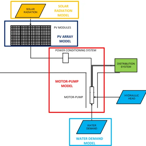
A PVWPS is basically composed of a PV array, a power controlling system and a pumping system connected to 131
the distribution system that can be a water tank or directly an irrigation system. A schematic diagram of the 132
photovoltaic water pumping system studied in this work and the related models adopted is presented in Figure 1. 133
The photovoltaic array consists of photovoltaic modules that are connected in series or in parallel depending on 134
the voltage and current output requirements. In this work both fixed and two-axis sun tracking systems were 135
investigated and compared technically and economically. The power controlling system is an interface between 136
the PV modules and the motor-pump system with the function to improve the coupling performances. The power 137
conditioning system can be a DC/DC converter or a DC/AC inverter depending on the motor-pump technology. 138
Both converter and inverter are usually equipped with a maximum power point tracker (MPPT) device in order to 139
maximize the power extraction from the solar array. In this study, both multistage centrifugal DC and AC pump 140
and the related power controllers were adopted in order to investigate and compare the performances, especially 141
in terms of power consumption, water pumped and costs. 142
143
Figure 1: Schematic diagram of a photovoltaic water pumping system. 144
3. METHODOLOGY
145
This study is divided into three parts: the estimation of the water demand for irrigation, the assessment of the 146
exploitable solar energy and related power output from the PV array, and sizing and dynamic modeling of the 147
system. The assessment of water demand depends on a lot of factors such as the type of crop, type of soil, 148
irrigated area, rainfall regime, average temperatures, wind speed and solar radiation. Here the FAO Penman-149
Monteith method was used to estimate the water demand for growing Alfalfa (Medicago Sativa) in a sandy soil 150
with some assumptions regarding the soil characteristics [5]. Based on this model both the assessment of the 151
monthly water demand that is the input data for the design procedure, and the hourly water demand used in the 152
dynamic modeling can be obtained. The assessment of the solar energy available and power output from the 153
solar array was made on the basis of data provided by a global climatic database and processed by the program 154
WINSUN considering different tilt angles and system configurations [7, 8]. The design process was carried out 155
through the estimation of the water demand and hydraulic head for growing Alfalfa in order to estimate the 156
power of the pumping system. The PV array power peak was then calculated on the basis of the daily required 157
hydraulic energy, daily collectable solar energy and system efficiency. The worst conditions in terms of available 158
solar energy and required water demand were chosen for the design procedure. The dynamic modeling of the 159
photovoltaic water pumping system was used to prove and optimize the sizing process, underlining the match 160
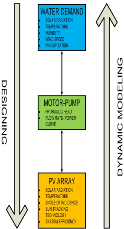
between water demand and water supply. A describing flow chart of the designing process and dynamic 161
simulations carried out in this paper and the related parameters affecting both processes are presented in Figure 162
2. 163 164
Figure 2: Designing and dynamic modeling procedure. 165
166 167
The dynamic simulations were done based on the hourly data of solar radiation, angle of incidence and 168
temperature in order to estimate the hourly power output from the PV array. The PV power output was then 169
used to estimate the hourly water output of the pumping system according to the power input-instantaneous 170
flow characteristic curve of the chosen pumps and power controller efficiency. The match between water supply 171
focused on the differences in initial capital costs between system equipped with AC and DC pump, fixed PV array 174
and sun tracking array. The economic investigation was based on the prices referring to the Chinese market and 175
taken from an on-line business-to-business trading platform [15]. 176
3.1 Climatic data
177
The site chosen for this study was in Xining, the capital city of Qinghai Province, China, located on the eastern 178
edge of the Qinghai-Tibet Plateau (Latitude: 36°37′ N; Longitude: 101°46′ E; Altitude: 2275 m a.s.l.). This location 179
is featured by a continental cold semi-arid climate with high potential in solar energy. The monthly daily average 180
temperatures range from -6.0°C in January up to 22.2°C in July. The annual precipitation is 269 mm and is mainly 181
distributed between May and September. The annual global radiation on horizontal plane is 1542 kWh/m2 with 182
2701 sunshine hours. The climatic data referring to Xining were taken from the global database provided by 183
Meteonorm including temperature, relative humidity, precipitation, wind speed, global radiation on a horizontal 184
plane, extraterrestrial radiation, incoming and outgoing longwave radiation as given in Table 1 [7]. The monthly 185
statistical data were used for the estimation of the monthly average daily water demand and the sizing of the 186
PVWPS. Whereas the hourly data elaborated by the software applying stochastic method were used for the 187
dynamic modeling of the water requirements and the photovoltaic pumping system. 188
189
Table 1: Climatic data for Xining. 190
3.2 Water demand
191
The model adopted for the estimation of the water demand was based on assumptions regarding the crop and 192
soil characteristics. In this study Alfalfa was chosen as growing crop whereas the characteristics of the ground 193
referred to a sandy soil. Both characteristic parameters of the growing crop and soil used in this model and 194
equations for the assessment of both average daily water requirements were taken from guidelines provided by 195
FAO [5]. The reference evapotranspiration was estimated through the method FAO Penman-Monteith that is a 196
procedure based on the climatic data of the site chosen for the irrigation system. 197
The daily trend of the reference evapotranspiration ET0 was calculated taking into account the monthly average
198
daily climatic data regarding solar radiation, temperature, humidity, vapor pressure and wind speed through the 199
following equation: 200
201
Where, Δ is the slope of the vapour pressure curve, Rn is the daily net radiation at the crop surface, G is the soil
202
heat flux density, γ is the psychrometric constant, es is the saturation vapor pressure,ea is the average daily actual
203
vapor pressure and u2 is the average monthly daily wind speed. The net radiation can be estimated as difference
204
between the incoming net shortwave radiation and the net outgoing longwave radiation. Based on the hourly 205
data of the involved parameters, the hourly water demand can be calculated from Equation 1 adjusted for one 206
hour time step. 207
The evapotranspiration in standard cultural conditions, ETc, was estimated from the reference value on the
208
basis of the growing crop, climatic conditions, and soil characteristic parameters and the vegetative phase. These 209
previous considerations are summed up in the cultural coefficient Kc. Then, ETc is given by:
210 211
In the specific case of Alfalfa Kc varies from 0.4 to 0.95 depending on the growing phase of the crop: Kc equal to
212
0.4 in development phase, 0.95 during the intermediate phase and 0.9 in the final phase. The development phase 213
runs from the sowing to the effective full ground cover, the intermediate stage from the effective full cover up to 214
the crop ageing and the final stage from the ageing up to the harvesting. In order to size the system, in this study 215
Kc was assumed equal to 0.95. The daily gross water volume needed by the crop Wg in mm/day can be estimated
216
taking into account evapotranspiration in the standard cultural conditions, effective rainfall, potential application 217
efficiency (PAE) and leaching requirement (LR). The gross water volume in mm/day is given by the following 218
equation: 219
220
where Pe is the effective rainfall, which was estimated from the monthly precipitation data by applying the Soil
221
Conservation Service (SCS) method developed by the United States Department of Agriculture [16]. In this 222
equation, LR implies the amount of water needed in order to remove residual salts from the root zone whereas 223
PAE refers to the efficiency of the irrigation plant. LR and PAE were set equal to 0.18 and 0.8 correspondingly, 224
when assuming to use a micro irrigation system. 225
Another important parameter for PVWPS is the irrigation turn that permits the planning of the irrigation. The 226
irrigation turn was estimated as the ratio between the amount of water released during an irrigation turn, Wt, and
227
the daily gross water volume. Wt represents the maximum water volume that the crop can absorb without water
228
losses. It depends on the water fraction absorbed by the crop, the wet surface due to the irrigation system, the 229
roots depth and the soil water content [17]. 230
The sizing of the system was based on the monthly average daily water demand, whereas the dynamic 231
modeling was based on hourly values. The estimated hourly water demand was then compared with the hourly 232
water supplied by the PV pumping system. Comparisons between water demand and water supply were made 233
also considering a time step equal to the irrigation turn and on monthly basis for the whole season. 234
3.3 Photovoltaic array
235
The power output provided by the PV array varies especially due to the different conditions of solar radiation 236
and temperature. Indeed those previous parameters affect the characteristic curve of the PV modules. The 237
dynamic modeling of the PV system considered the estimation of the hourly power output of the solar array 238
P(T,θ), depending on the hourly beam radiation Ib and diffuse radiation Id, incidence angle θ and temperature T.
239
The following equation was used to evaluate the hourly power output from 1 kWp PV array [18]:
240 241
Where η0b is the optical efficiency for the beam radiation, Kb(θ) is the incidence angle modifier, Kd is the incidence
242
modifier for diffuse radiation Tc is the cell temperature, Tr is the reference temperature (25°C) and α is the power
243
temperature coefficient. The first term of Equation 4 represents the power output from 1 kWp PV modules at the
244
reference temperature, whilst the second term accounts for the power losses due to temperature deviation from 245
the reference value. The influence of the temperature on the PV modules performance was taken into account 246
through the cell temperature Tc that is affected by the ambient temperature Ta and the global solar radiation Itot
247
trough the following equation: 248
249
Where, NOCT is the nominal operating cell temperature. Simulations of the power output from the PV array were 250
conducted with WINSUN that is software based on TRNSYS system simulation [9]. The dynamic modeling of the 251
solar array power output was estimated taking into account the hourly values of beam radiation, diffuse 252
radiation, incidence angle and ambient temperature. The calculations carried out with WINSUN considered the 253
effects of both optical efficiencies and angle modifiers, whereas the effect of the temperature was estimated 254
separately through a MATLAB script. Both fixed array and fully tracking array were investigated in this work. The 255
sizing of the PV water pumping system was carried out through a simple approach based on the daily hydraulic 256
energy Eh required to lift the water demand, the average daily radiation on the plane of the array Itot,d and the
257
overall system efficiency ηs. This approach is summed up in the following equation [19]:
258
259
The daily hydraulic energy was estimated from the daily water demand and hydraulic head with the following 260
formula: 261
Where ρ is the water density and g is the gravity acceleration. In Equation 7 Wg is expressed in m3/ha day (1
263
mm/day corresponds to 10 m3/ha day). The efficiency of the system takes into account the efficiency of the MPPT 264
system, controller or inverter, electric engine, centrifugal pump and system losses [20, 21]. 265
3.4 DC/DC converter-motor-pump
266
The model used in this work for the converter and inverter was based on the assumption that the output power 267
is equal to the input power from the photovoltaic generator less the unavoidable power losses associated. 268
Normally the efficiency varies between the 80% up to the 95 % depending on working conditions, especially 269
temperature, and power available. The power losses were taken into account on the basis of an average 270
efficiency of the power controlling system. 271
The motor-pump was sized on the basis of instantaneous water flow, estimated from daily water demand and 272
daily operating hours, and hydraulic discharge. The total dynamic head was calculated taking into account several 273
contributions such as outlet minimum pressure required by the irrigation system, height of the of the outlet pipe 274
above the ground surface, depth of the static water level, depth of the dynamic water level and friction losses due 275
to the pipeline circuit. In this study a hydraulic discharge measured in field tests was used. The sizing of the 276
centrifugal motor-pump in kW was carried out with the following equation: 277
278
Where, Q is the flow expressed in m3/s, 1000 is a conversion factor and ηp is the efficiency of the motor pump
279
system. 280
The motor-pump system was modeled on the basis of the governing equations of the electric engines, affinity 281
laws and hydraulic power. The main input data regarding the minimum and maximum head and the 282
corresponding flows and efficiencies, were taken from motor-pump datasheet provided by pumps manufacturer 283
companies [22, 23]. The dynamic modeling of the pump was carried out considering the pump characteristic 284
curve that expresses the instantaneous water flow in m3/h versus the hourly feeding power to the motor-pump 285
system. A typical expression of the relationship between water flow Q, hydraulic discharge H and power input Pin
286
is given by the following third grade polynomial: 287
288
Where, c1, c2, c3 and c4 are experimental coefficients. The previous curves, both for the DC and AC pump, were
289
obtained from PVsyst (v5.55) through the specific tool for pumping system and adjusted with the curve fitting 290
function in MATLAB. 291
4. RESULTS AND DISCUSSIONS
292
This section shows the results regarding the assessment of water demand and solar energy, sizing and modeling 293
of the system, matching between water demand and water supply and economics analysis between DC and AC 294
pump and fixed and fully tracking PV array. In this work an irrigated area of 1 ha was considered. 295
4.1 Assessment of the water demand
296
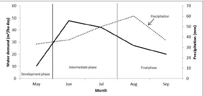
The monthly average water demand for the growing of Alfalfa on a sandy soil and the trend of the monthly 297
average precipitation are presented in Figure 3. 298
299
Figure 3: Monthly average daily water demand. 300
301
It is clear that the trend of the daily water demand for irrigation is affected mainly by the evaporation related to 302
the growing phase and rainfall. The evapotranspiration registered a peak during the sunniest months of the year 303
whereas the precipitation registered the highest values in the period May-September. The irrigation season for 304
the crop chosen is five months, this study interested then only the months from May to September. In this work it 305
was assumed that in May takes place the development phase, in June and July the intermediate phase and in 306
August and September the final phase. The Alfalfa water demand trend shows then a peak during the month of 307
June of 47 m3/ha and it decreases during the remaining months. The minimum daily water demand estimated for 308
this period corresponded to the water requirements in May which is equal to 10.4 m3/ha. The irrigation turn 309
estimated by the model was 10 days. In this work an irrigated area of 1 ha was considered. The validation of the 310
results obtained from the water demand model was carried out through personal communication with field 311
expert and with the results obtained in field studies conducted in the same region [24]. The former proved that 312
the daily maximum water requirement for irrigation is 50 m3/ha. Whereas the results obtained in previous field 313
studies showed an irrigation duty of 600 m3/ha for an irrigation turn of 14 days corresponding to 40 m3/ha day. 314
4.2 Solar energy assessment
315
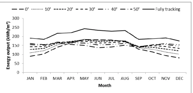
The available solar radiation and its variation with the tilt angle and system technology are shown in Figure 4. In 316
this study it was assumed to use a fixed system with an azimuth angle equal to 0° that corresponds to solar array 317
oriented towards south. The results of the simulations show that for the fixed system the best tilt angle on annual 318
basis was 30° with a corresponding collectable solar radiation of 1870 kWh/m2 year. For the simulations carried 319
out only during the irrigation season, from May to September, the best tilt angle resulted in 10° collecting 854 320
kWh/m2 season. The 10° tilted solar array was then used in our study. As regards the fully tracking system, the 321
annual collected solar radiation on the plane surface was 2490 kWh/m2 year whereas 1120 kWh/m2 during the 322
irrigation season. This corresponds to a collected solar energy 30 % higher compared to the optimal fixed system. 323
324
Figure 4: Solar energy available depending on the tilt angle and system technology. 325
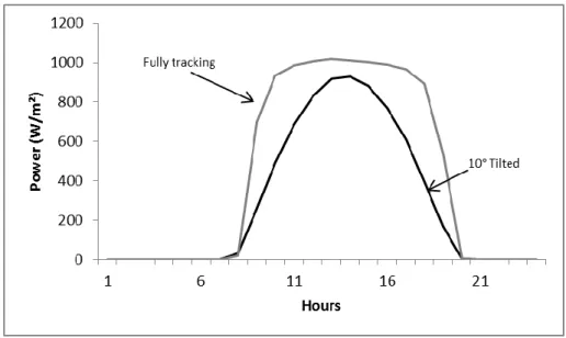
The power output from fixed and fully tracking PV system with a capacity of 1 kWp during a sunny day in June is
326
shown in Figure 5. The energy collected by the 10° tilted system was 7.0 kWh/m2 whereas the solar energy 327
collected by the fully tracking array it was equal to 10 kWh/m2 corresponding to 40% more energy than the fixed 328
system. The better performances of the sun fully tracking system are mainly due to the system, varying 329
continuously its tilt and azimuth angle in order to follow the sun, optimizes the harnessing of available solar 330
radiation guaranteeing a wider range of working hours at higher power output compared to the fixed system. 331
332
Figure 5: 1 Kwp power output during a sunny day in June. 333
334
It is clear that the solar generator power output depends on the variation of the available solar power and is 335
mainly sensitive to the variation of ambient temperatures. The typical effect of the hourly variation of ambient 336
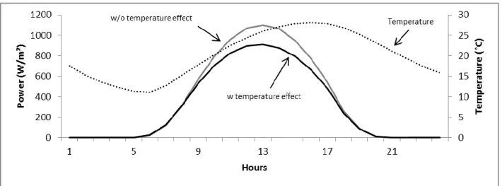
temperature on the power output of solar array is presented in Figure 6 for 1 kWp PV array.
337 338
Figure 6: Effect of the temperature on the power output of 1 kWp solar array. 339
340
The power output from the solar generator without considering the temperature effect, is the power at the 341
reference temperature of 25 °C and depends only on the available solar radiation, PV modules optical efficiency 342
and incidence angle modifiers. As it is shown, the temperature affects the power generation of the solar array 343
during the sunniest and warmest hours of the day due to the difference between cell temperature and reference 344
temperature. The maximum drop of the efficiency and the subsequent drop of power generation were registered 345
at 1 pm and it was equal to 198 W representing a loss of 17 %. The high value of power waste was due to the 346
theoretical approach used in this study to perform the effect of temperature on the PV modules efficiency. The 347
previous approach tends to overestimate the power losses due to temperature, usually in the range of 10 %, on 348
behalf of guaranteeing more accurate water supply forecasts. 349
4.3 Pump modeling
350
The sized PV systems were used in dynamic simulations in order to estimate the hourly power output and hourly 351
water pumped. The dynamic modeling of the photovoltaic pumping system could further verify if the sized system 352
could fulfill the dynamic water requirements. The water pumped under different PV power output was estimated 353
on the basis of the pump characteristic curve flow rate against power input. Obviously, the instantaneous 354
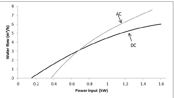
pumped water flow is mainly affected by the variation of the power coming from the solar array. Figure 7 shows 355
the instantaneous water flow at different motor power input. 356
357
Figure 7: Instantaneous water flow compared to the power input to the motor. 358
In the case of the AC technology the engine starts to drive the pump when is reached a minimum feeding power 360
of 0.37 kW. The instantaneous flow increases with the input power until reaching 1.5 kW. The motor-pump speed 361
is governed in the above mentioned power range following the pattern outlined. For input power greater than 1.5 362
kW the speed and then the water output was kept constant and equal to the maximum due to the power 363
conditioning system interface in order to avoid damages to the electric engine. In the case of the DC motor the 364
power working range varies from 0.15 kW and 1.6 kW. 365
4.4 Sizing of the system
366
The sizing of PV array and pump was then made on the basis of the water demand, total dynamic head, solar 367
energy available and efficiencies of the system. The system was sized on the basis of the worst month marked out 368
by the lowest ratio between monthly daily average solar radiation and monthly daily average water demand, as 369
shown in Table 2. 370
371
Table 2: Solar energy and water demand ratio. 372
373
June presented the lowest ratio between daily solar radiation and water demand especially due to the highest 374
water requirements registered during the irrigation period. June was then chosen as designing month. According 375
to the estimation of water demand, 47.1 m3 of water is needed every day during the irrigation turn. The PV array 376
peak power was estimated on the basis of the daily hydraulic energy required to achieve a hydraulic head of 40 m 377
and the monthly average daily solar radiation. The resulting required hydraulic energy was 5 kWh/day whereas 378
the resulting monthly average daily solar radiations were 6.0 kWh/m2 and 7.8 kWh/m2 for fixed system and fully 379
tracking system respectively. The sizing procedure for the PV array peak power is also affected by the efficiencies 380
of controller or inverter, electric engine, pump and other unavoidable system losses due mainly to power losses 381
of PV modules affected by temperature variation and electric losses in the wires. All these contribution are 382
summarized in the overall system efficiency ηs given by the following:
383 384
Where ηpc is the efficiency of the power conditioning system, ηp is the efficiency of the pumping system and ηPV,T
385
and ηw consider the losses power losses in the PV modules and wires. These efficiencies vary with device models
386
and working conditions. For example, the efficiency of the power conditioning system is affected mainly by the 387
power input and ambient temperature varying between 80 % and 95 %, the motor pump efficiency varies from 40 388
% up to 60 % depending on power input, water flow and pressure. In this study, in order to take into account the 389
effect of components efficiency on the system performances, three values of the system efficiency were tested in 390
the design and subsequently proved through dynamic simulations: 30%, 35% and 40% respectively. This resulted 391
in three different PV array sizes for both fixed and fully tracking installation. The resulting PV array power were 392
2.8 kWp, 2.4 kWp and 2.1 kWp for the fixed system and 2.1 kWp, 1.8 kWp and 1.6 kWp for the two-axes tracking
system respectively. On the basis of the power peak obtained, the corresponding PV area was estimated 394
assuming an energy conversion efficiency of the PV panels equal to 14.3 % [25]. The pump capacity was estimated 395
according to the hydraulic head and the instantaneous water flow. The instantaneous water flow was estimated 396
from the daily water demand assuming 8.5 operating hours. The required pump power resulted in 1.5 kW. 397
According to the pumps available on the market, the following pumps were adopted: 1.6 kW DC centrifugal 398
multistage and 1.5 kW AC single phase centrifugal multistage. The main input data and results of the designing 399
phase are summarized in Table 3. 400
401
Table 3: Summary of the main system parameters and sizing results. 402
403
4.5 Design proving
404
Concerning the worst situation in June, the simulated pumped water was compared with the estimated daily 405
water demand in order to identify the mismatches. The simulation step was set equal to the irrigation turn, 10 406
days, period marked out by a water demand of 470 m3. 407
As the motor-pump system was driven by a 2.8, 2.4 and 2.1 kWp fixed PV arrays, the pumped water during the
408
first irrigation turn in June amounted to 515, 470 and 426 m3 respectively when using the DC pump; while 599, 409
531 and 470 m3 respectively when using the AC pump. Therefore, the system of AC pump can always satisfy the
410
water demand. However, for the system of DC pump centrifugal pump, it has to be driven by a PV array larger 411
than 2.4 kWp in order to achieve the pumped water could match the water demand. For the case of DC
412
centrifugal pump driven by 2.1 kWp PV array the mismatch was 44 m3. The achieved results through dynamic
413
simulations for the fixed PV systems are presented in Figure 8. 414
415
Figure 8: Pumped water flow during an irrigation turn in June with fixed PV array. 416
417
As the solar arrays mounted on the two-axis tracking system, the amounts of pumped water in June were 418
calculated as 546, 492 and 448 m3 for the 2.1, 1.8 and 1.6 kWp respectively when using DC pump; while 634, 553
419
and 486 m3 respectively when using AC pump. It is similar the situation of fixed PV system that the system of AC 420
pump can always satisfy the water demand. For the system of DC pump, the PV array has to be larger than 1.8 421
kWp. The better performances of the AC pump compared with the DC were mainly due to the specific
422
characteristic curve power input against instantaneous water flow. Although the DC pump is marked out by a less 423
required power input to start running the pump and a higher rated power compared to the AC pump, the latter is 424
featured by a higher water flow output for input power greater than 0.7 kW resulting in greater volume of water 425
pumped. The dynamic simulations results for the sun tracking PV systems are presented in Figure 9. 426
429
It is clear that the overall efficiency used in the sizing phase affected the amount of pumped water. The 430
achieved results show that a suitable design of the DC pumping system driven by the fixed PV array is based an 431
overall efficiency of both 30% and 35%. These efficiencies permitted during the dynamic simulation to achieve the 432
amount of water needed for the irrigation purposes. Efficiency equal to 35 % permitted to both fulfill the water 433
requirements and minimize the PV modules area optimizing the system. Even in the case of DC pumping system 434
driven by the fully tracking PV array, both 30% and 35% were suitable efficiencies for the designing of the system. 435
In the case of the AC pump powered by the fixed solar array, the optimization of the system was achieved by an 436
efficiency of 40 % considered during the design process both for the fixed and fully tracking PV array. It has to be 437
pointed out that it doesn’t imply that the high system efficiency is not desirable. The reason that the high 438
efficiency system (40%) has a worse performance is mainly due to that the efficiency considered in the design 439
stage is a based on steady performance. However, in order to represent the dynamic characters of both the 440
climatic conditions and the system components, dynamic efficiencies may be required. Therefore, it is of great 441
importance to conduct the dynamic simulation to prove the design and find the optimal value. Meanwhile, the 442
overall system that accounts for the components dynamic efficiencies and, as the achieved results show, the 443
optimal value can be set only through dynamic simulations need to be included in the future study to have a more 444
accurate simulation. 445
The water output simulations were extended to the whole irrigation season as well, from May to September, 446
comparing the crop variable water demand depending on the growing phase with the variable water supply due 447
to the variation of available solar energy. Both DC and AC pump technology and optimal fixed and sun tracking 448
array were used in these simulations. The monthly results about water demand and water supply are shown in 449
Figure 10. Since that the water pumping system was sized for the worst month, there was then a surplus of 450
pumped water during the months featured by a higher solar energy and water demand ratio than the 451
corresponding designing month. Indeed, the water demand for Alfalfa varies during the irrigation season 452
depending on the crop growing period. Simultaneously the available solar radiation varies during the irrigation 453
season affecting the power output and then the pumped water. 454
455
Figure 10: Monthly water demand and supply estimated through dynamic simulations. 456
457
Moreover, when extending the simulations to one month instead of within one irrigation turn (ten days), some 458
critical situations occur. It is clear from Figure 10 that both DC and AC driven by tracking PV array could fulfill the 459
water requirements in June. However, when fixed PV array is used, some mismatching between water supply and 460
water demand were identified: 13 m3 for the DC pump system driven by 2.4 kWp PV array and 24 m3 for the AC
461
pump system driven by the 2.1 kWp PV array. The mismatching identified in the monthly simulation was the result
462
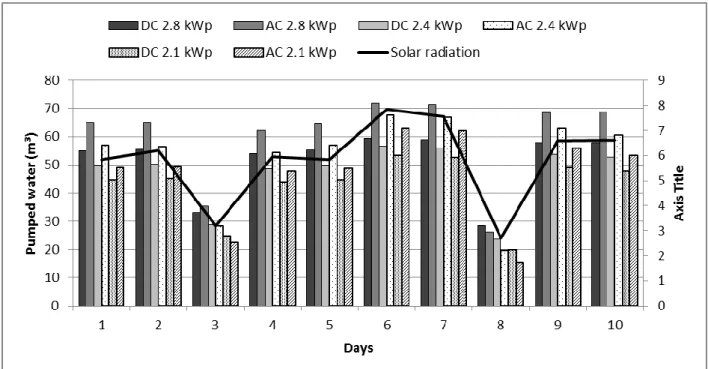
of the dynamic variability of solar radiation affecting the water output from the pumping systems. As shown in 463
Figure 11, days marked out by poor solar energy conditions can considerably affect the amount of pumped water 464
but without substantially affecting the water demand since the latter depends on more climatic parameters, such 465
as humidity, wind and rainfall. Moreover, in periods or months marked out by lower solar energy, such as 466
September, systems using DC pump technology offered better performances in terms of water supply due to the 467
lower power input requirements. 468
The surplus of pumped water recorded during the irrigation season could be used in order to extend the 469
irrigated area or for other purposes in order to use the system more effectively. For example, if the surplus of 470
water is used for irrigation, for the AC pump system driven by the 1.6 kWp PV tracking array, the irrigated area can
471
be extended up to 4.9 ha when it is in May and 1.7 ha in August and September; while for the DC pump system 472
driven by 1.8 kWp PV tracking array, the irrigated area can be extended to 4.7 ha in May and 1.7 and 1.8 in August
473
and September respectively. 474
475
Figure 11: Hourly dynamic simulations of water demand and water supply from AC pump powered by 2.1 kWp solar 476 array. 477 478 4.6 Economic analysis 479
An economic analysis based on the investment costs was carried out in order to investigate the most cost 480
effective solution among the alternatives presented in this study especially between system equipped with fixed 481
and sun tracker array and AC and DC pump technology. This analysis was performed in order to combine both 482
economic aspects and performances in terms of water pumped according to the crop water requirements 483
previously discussed. 484
The prices of the PV modules are highly variable depending on the market and the manufacturer company. 485
Nevertheless it represents one of the major costs for a photovoltaic pumping system, accounting for more than 486
the 30 % of the overall costs (considering in the economic analysis the cost of well digging). Using the sun tracking 487
system permits a smaller area of PV modules which resulted in a deducted capital cost of PV cells and power 488
conditioning system. But at the same time the tracker can highly contribute on the overall cost of the system 489
mainly due to its high accuracy technology. Moreover, DC pump are more expensive compared to AC pump but 490
on the contrary the controller used as interface between the PV modules and the DC electric engine is more 491
affordable then DC/AC inverter. Comparing the 1.8 kWp two-axis tracking system with the 2.4 kWp fixed solar
492
array powering the DC pumping system, although the tracking system has a power peak about 30% less than the 493
fixed system, the former offers better performances than the latter due to the daily higher exploitability of solar 494
energy. The AC pump driven by the fixed 2.1 kWp PV array fulfilled the water requirements as the DC pump
495
powered by the fixed 2.4 kWp solar generator saving 0.3 kWp of solar cells. Even the AC pumping system powered
installation of 0.8 kWp of solar cells compared to the DC 2.4 kWp fixed system and 0.5 kWp of PV modules
498
compared to the AC 2.1 kWp fixed system.
499
The PVWPS systems compared in terms of initial investment costs (IIC) in this economic analysis were the same 500
systems compared in terms of water pumped in the previous section of this paper. The possibility to install 501
tracking system instead of fixed system and DC instead of AC pump was estimated. All the prices used in the 502
investigation, summarized in Table 4, were taken from a business-to-business online platform and refer to the 503
Chinese market [16]. 504
505
Table 4: PV water pumping system components unit costs. 506
507 508
The results of the economic analysis are presented in Figure 12, outlining the total initial capital cost together 509
with the costs contributions. 510
511
Figure 12: Total initial investment costs for the PVWPS proposed. 512
513
On the basis of the economic investigation carried out, the most cost effective solution was the AC 2.1 kWp
514
fixed system with an overall initial capital cost of 2450 $ followed by the DC 2.4 kWp system marked out by an
515
initial capital cost of 2950 $. The reason that the DC fixed system has a higher investment compared with the 516
corresponding AC fixed system was mainly due to the cost difference of DC and AC pump, 640 $ against 150 $, 517
rather than the cost difference of PV modules, 1440 $ against 1260 $. Despite of the reduction in cost due to the 518
installation of DC/DC converter on behalf of the installation of DC/AC inverter, the AC fixed system was the most 519
cost-effective solution. Comparing the fixed system with the corresponding systems equipped with the sun 520
tracker device, the formers presented lower investment cost than the latter especially because of the high 521
investment cost due to the tracking system. The tracked DC 1.8 kWp system had an investment cost of 4350 $ of
522
which 1620 $ were due to the sun tracking device accounting for 37 % of the overall cost. The cost reduction due 523
to the lower investment in PV modules and power conditioning system using sun tracking technology had no 524
positive effects. A possible application of PVWPS equipped with solar tracker could be economically supported in 525
the case the system is used for multipurpose applications during the months where the irrigation is not needed. 526
5. CONCLUSIONS
527
In this study a dynamic simulation tool combining the models of the water demand, the solar PV power and 528
pumping system was developed in order to be used for quick design and design validation. According to the 529
achieved results the following conclusion can be pointed out: 530
The sizing of photovoltaic water pumping systems for irrigation is extremely affected by the dynamic 531
character of the water demand and collectable solar energy. In order to define the worst condition on 532
the basis of which the system is sized, the lowest ratio between required hydraulic energy and available 533
solar radiation has to be considered. 534
The assessment of the overall system efficiency ηs is relevant to optimally size the PV array power peak
535
avoiding both system failure and economic losses. ηs summarizes in a steady value the dynamic
536
efficiency of the system components and the optimal value can only be set through system dynamic 537
simulations verifying the match between pumped water and water demand. 538
Preliminary economic analysis based on the initial investment costs showed that AC pump powered by 539
fixed PV array represent the most cost-effective solution for water pumping. 540
ACKNOWLEDGEMENTS
541
The authors are grateful to the Swedish International Development Cooperation Agency (Project No.: AKT-2010-542
040) for the financial support. 543
REFERENCES
544
[1] Argaw N, Foster R, Ellis A. Renewable Energy for Water Pumping applications in rural villages. NREL. 2001. 545
[2] IEA, Policy recommendations to improve the sustainability of rural water supply systems. Report IEA-PVPS T9-546
1:2011. 547
[3] IEA, 16 Case studies on the deployment of photovoltaic technologies in developing countries. Report IEA-PVPS 548
T9-07:2003. 549
[4] IEA,Trends in photovoltaic applications survey report of selected IEA countries between 1992 and 2010, 550
Report IEA-PVPS T1-20:2011. 551
[5] Allen RG, Pereira LS. Raes D, Smith M. Crop evapotranspiration. Guidelines for computing crop water 552
requirements. FAO. 1998. 553
[6] Bouzidi B, Haddadi M, Belmokhtar O. Assessment of a photovoltaic pumping system in the areas of the 554
Algerian Sahara. Renewable & Sustainable Energy Reviews 2008. 13: 879-886. 555
[7] Meteonorm, http://meteonorm.com/, 2012-01-30. 556
[8] Perers B, Karlsson B. Energy and building design. Lund University, Faculty of Engineering (LTH); 2007. WINSUN 557
Based on TRNSYS/TRNSED/PRESIM 14.2. 558
[9] Castaner L, Silvestre S. Modelling photovoltaic systems using PSpice®. 1st ed. UK: Wiley. 2002. 559
[10] Hsiao YR. Direct coupling of photovoltaic power source to water pumping system. Solar Energy 1983. 32(4): 560
489-498. 561
[11] Hamidat A, Benyoucef B. Systematic procedures for sizing photovoltaic pumping system using water tank 562
storage. Energy Policy 2009. 37: 1489-1501. 563
[12] Bakelli Y, Arab AH, Azoui B. Optimal sizing of photovoltaic pumping system with water tank storage using 564
[13] Ould-Amrouche S, Rekioua D, Hamidat A. Modelling photovoltaic water pumping system and evaluation of 566
their CO2 emissions mitigation potential. Applied Energy 2010. 87: 3451-3459.
567
[14] Fedrizzi MC, Ribeiro FS, Zilles R. Lessons from field experiences with photovoltaic pumping systems in 568
traditional communities. Energy for Sustainable Development 2009. 13: 64-70. 569
[15] Alibaba, http://www.alibaba.com/, 2012-08-30 570
[16] United States Department of Agriculture, Natural Resources Conservation Service, 571
http://www.nrcs.usda.gov/wps/portal/nrcs/main/national/home, 2012-02-01. 572
[17] A. Capra, B. Scicolone, “Project and management of irrigation plant-Criteria for the use and exploitation of 573
water for irrigation purpose”. 2007. 1st ed. Edagricole. (In Italian) 574
[18] J. A. Duffie, W.A. Beckman. Solar Engineering of Thermal Processes. 3rd ed. 2006. Wiley. 575
[19] S. R. Wenham, M. A. Green, M. E. Watt, R. Corkish, “Applied photovoltaics”, Second Edition, Earthscan 576
[20] Khatib T. Design of photovoltaic water pumping system at minimum cost for Palestine: a review. Journal of 577
applied sciencies 2010. 10 (22): 2773-2784. 578
[21] Lynn PA. Electricity from sunlight. 1st ed. UK: Wiley. 2010. 579
[22] Lorentz, http://www.lorentz.de/, 2012-01-30. 580
[23] Matra, http://www.matra.it/, 2012-01-30. 581
[24] Final report. ADB RSC-C91300 (PRC). Qinghai Pasture Conservation Using Solar Photovoltaic (PV)-Driven 582
Irrigation. 2010. 583
[25] Schott, www.schottsolar.com/ global/ products/ photovoltaics/ schott-poly-245/, 2012-02-14 584 585 586 587 588 589 590 591 592 593 594 595 596 597 598 599 600
Figure captions
601
Figure 1: Schematic diagram of a photovoltaic water pumping system. 602
Figure 2: Designing and dynamic modeling procedure. 603
Figure 3: Monthly daily estimated water demand. 604
Figure 4: Solar energy available depending on the tilt angle and system technology. 605
Figure 5: 1 Kwp power output during a sunny day in June.
606
Figure 6: Effect of the temperature on the power output of 1 kWp solar array.
607
Figure 7: Instantaneous water flow compared to the power input to the motor. 608
Figure 8: Pumped water flow during an irrigation turn in June with fixed PV array. 609
Figure 9: Pumped water flow during an irrigation turn in June with tracking PV array. 610
Figure 10: Monthly water demand and supply estimated through dynamic simulations. 611
Figure 11: Hourly dynamic simulations of water demand and water supply from AC pump powered by 2.1 kWp
612
solar array. 613
Figure 12: Total initial investment costs for the PVWPS proposed. 614 615 616 617 618 619 620 621 622 623 624 625 626 627 628 629 630 631 632 633
SOLAR RADIATION HYDRAULIC HEAD WATER DEMAND DISTRIBUTION SYSTEM PV MODULES
POWER CONDITIONING SYSTEM
MOTOR-PUMP MOTOR-PUMP MODEL PV ARRAY MODEL WATER DEMAND MODEL SOLAR RADIATION MODEL 636
Figure 1: Schematic diagram of a photovoltaic water pumping system. 637 638 639 640 641 642 643 644 645 646 647 648 649 650 651 652 653 654 655
WATER DEMAND SOLAR RADIATION TEMPERATURE HUMIDITY WIND SPEED PRECIPITATION D E S I G N I N G D Y N A M I C M O D E L I N G MOTOR-PUMP HYDRAULIC HEAD
FLOW RATE- POWER CURVE PV ARRAY SOLAR RADIATION TEMPERATURE ANGLE OF INCIDENCE SUN TRACKING TECHNOLOGY SYSTEM EFFICIENCY 656 657
Figure 2: Designing and dynamic modeling procedure. 658 659 660 661 662 663 664 665 666 667 668 669 670 671 672 673 674 675 676
679
Figure 3: Monthly average daily water demand. 680 681 682 683 684 685 686 687 688 689 690 691 692 693 694 695 696 697 698 699 700 701 702 703 704 705
706
Figure 4: Solar energy available depending on the tilt angle and system technology. 707 708 709 710 711 712 713 714 715 716 717 718 719 720 721 722 723 724 725 726 727 728 729 730 731
734
Figure 5: 1 Kwp power output during a sunny day in June. 735 736 737 738 739 740 741 742 743 744 745 746 747 748 749 750 751 752 753 754 755 756 757 758 759 760 761
762
763
Figure 6: Effect of the temperature on the power output of 1 kWp solar array. 764 765 766 767 768 769 770 771 772 773 774 775 776 777 778 779 780 781 782 783 784 785 786 787 788
792
793
Figure 7: Instantaneous water flow compared to the power input to the motor. 794 795 796 797 798 799 800 801 802 803 804 805 806 807 808 809 810 811 812 813 814 815 816 817 818
819
820
Figure 8: Pumped water flow during an irrigation turn in June with fixed PV array. 821 822 823 824 825 826 827 828 829 830 831 832 833 834 835 836 837 838 839 840 841
845
846
Figure 9: Pumped water flow during an irrigation turn in June with tracking PV array. 847 848 849 850 851 852 853 854 855 856 857 858 859 860 861 862 863 864 865 866 867 868 869 870
871
Figure 10: Monthly water demand and supply estimated through dynamic simulations. 872 873 874 875 876 877 878 879 880 881 882 883 884 885 886 887 888 889 890 891 892 893 894 895
898
Figure 11: Hourly dynamic simulations of water demand and water supply from AC pump powered by 2.1 kWp solar 899 array. 900 901 902 903 904 905 906 907 908 909 910 911 912 913 914 915 916 917 918 919 920 921 922 923
924
Figure 12: Total initial investment costs for the PVWPS proposed. 925 926 927 928 929 930 931 932 933 934 935 936 937 938 939 940 941 942 943
Table captions
946
Table 1: Climatic data for Xining. 947
Table 2: Solar energy and water demand ratio. 948
Table 3: Summary of the main system parameters and sizing results. 949
Table 4: PV water pumping system components unit costs. 950 951 952 953 954 955 956 957 958 959 960 961 962 963 964 965 966 967 968 969 970 971 972 973 974 975 976 977
Table 1: Climatic data for Xining. 978
Jan Feb Mar Apr May Jun Jul Aug Sep Oct Nov Dec
T (°C) -6.0 -2.0 5.0 11.6 16.8 19.8 22.2 21.1 15.5 9.7 1.9 -4.8 RH (%) 65.6 65.0 60.5 57.6 56.5 60.6 65.5 67.4 66.9 63.6 65.3 70.2 P (mm) 0.7 3 8.3 16 33.3 37.3 50 60.2 36.6 18.7 4.5 0 WS (m/s) 2.8 3.0 3.6 3.7 3.7 3.2 3.0 2.9 2.8 2.9 3.1 2.9 GH (kWh/m2) 75.6 96.6 144.3 168.5 182.2 187.2 184.5 157.7 127.5 89.3 76.1 53.5 EX (kWh/m2) 149.8 176.3 253.0 297.8 344.6 346.7 349.7 319.4 262.8 212.8 156.9 136.8 LI (kWh/m2) 160.9 156.4 195.4 210.8 239.0 247.2 269.0 267.1 235.9 219.5 184.0 170.6 LO (kWh/m2) 209.3 204.3 254.6 272.5 303.3 306.6 326.0 319.6 285.5 269.4 232.2 212.9 979 980 981 982 983 984 985 986 987 988 989 990 991 992 993 994 995 996 997 998 999 1000
Table 2: Solar energy and water demand ratio. 1003
May June July Aug Sept
Itot (kWh/m2day) 5.9 6.0 5.8 5.7 4.6 Wg (m3/ha day) 10.4 47.1 42.0 27.0 20.1 Ratio (%) 56.7 12.9 14.4 21.1 22.8 1004 1005 1006 1007 1008 1009 1010 1011 1012 1013 1014 1015 1016 1017 1018 1019 1020 1021 1022 1023 1024 1025 1026 1027 1028 1029 1030 1031
Table 3: Summary of the main system parameters and sizing results. 1032
Water demand (m3/ha/day) 47.1
Irrigated area (ha) 1
Daily operating hours 8.5
Total dynamic head (m) 40
Pump power (kW) 1.5
Average monthly daily solar radiation on fixed system (kWh/m2) 6.0 Average monthly daily solar radiation on tracking system (kWh/m2) 7.8
PV module efficiency in STC (%) 14.3
NOCT (°C) 47.2
Power temperature coefficient (%/°C) -0.45
Efficiency of the system (%) 30 35 40
Fixed system power peak (kWp) 2.8 2.4 2.1
Fixed system array area (m2) 20 17 15
Tracking system power peak (kWp) 2.1 1.8 1.6
Tracking system array area (m2) 15 13 11
1033 1034 1035 1036 1037 1038 1039 1040 1041 1042 1043 1044 1045 1046 1047 1048
Table 4: PV water pumping system components unit costs. 1051
Component Unit cost
PV modules 0.6 $/Wp Structure 0.1 $/Wp PV tracking system 0.9 $/Wp DC/AC Inverter 0.2 $/Wp DC/DC Converter 0.06 $/Wp AC pump 0.1 $/W DC pump 0.4 $/W
Engineering and installation 20 % (IC) 1052