Towards a New Classification of Rivers based on Generic Gage Height –
Discharge Rating Curves for Low-Cost Estimation of Stream Discharge
Jeremiah B. Rundall, Benjamin E. ParsonsDepartment of Physics, Utah Valley University, Orem, Utah Steven H. Emerman1
Department of Earth Science, Utah Valley University, Orem, Utah Michael R. Jorgensen
Department of Physics, Utah Valley University, Orem, Utah
Abstract. The objective of this research is to classify rivers based upon generic gage height-discharge rating curves so as to reduce the number of measurements required for rating curve development. The first step has been classification according to the uniqueness of the gage height-discharge relationship. The USGS National Water Information System database of 3.68 million pairs of gage height vs. discharge measurements at 61,240 gaging stations was imported into a Python-driven data manipulation script, resulting in 15,153 gaging stations after removal of incomplete and inconsistent data. At each gaging station, the linear relationship ZlnGH = mZlnQ + b
was determined, where ZlnGH and ZlnQ are the Z-scores of the logarithms of gage height and
discharge, respectively. Each linear relationship was converted into a normal distribution with mean and standard deviation equal to m and its standard error, respectively. Summation of the normal distributions showed a single peak at m = 0.991, where m = 1 indicates a unique gage height-discharge relationship. There are no gaging stations with m > 1, equivalent to no gaging stations with variation in discharge without variation in gage height. Over 30% of gaging stations had m < 0.9, indicating significant variation in gage height without variation in discharge. Based on 209 gaging stations in Utah, extreme independence of gage height from discharge (m < 0.6) can be avoiding by not locating gaging stations close to either the upstream or downstream confluence (within 10% of the reach), which precludes the effects of flood waves and reverse flow.
1. Introduction
A rating curve is an empirical relationship between gage height and stream discharge that is used to derive a hydrograph from a record of gage height. The development of a rating curve requires multiple simultaneous field measurements of gage height and discharge over a wide range of discharge values, so that rating curve development is a major manpower expense for state and federal agencies that monitor stream discharge. The objective of this research is to explore the possibility of a new classification of rivers based upon generic gage height-discharge rating curves with a small number of adjustable
parameters, so as to reduce the number of field measurements required to establish or maintain a gaging station.
An earlier study asked whether a generic rating curve could be assigned to a
sufficiently restricted class of rivers, such as bedrock step-pool rivers (Stuart and Emerman
1 Department of Earth Science
Utah Valley University Orem, Utah 84058 Tel: (801) 863-6864 e-mail: StevenE@uvu.edu
2012). However, the generic rating curve developed for 71 gaging stations on bedrock step-pool rivers was not a significantly better predictor for discharge from gage height than the generic rating curve developed for 71 randomly chosen rivers of all types (Stuart and Emerman 2012). That result raised the possibility that, at the present time, it is not known what observable aspects of rivers are critical for the choice of a rating curve in the absence of the conventional multiple measurements of gage height and discharge. Therefore, this study takes a “reverse engineering” approach of first asking what are the categories of existing rating curves and then asking what are the observable characteristics of the rivers that belong to those categories of rating curves.
Most recent work on rating curves has involved the development of rating curves based on channel geometry without any gage height vs. discharge measurements (Bailey 1966; Drus 1982; Davidian 1984; Jarrett and Malde 1987; Di Giammarco et al. 1998; Wilson et al. 2002; Gergov and Karagiozova 2003; Kean and Smith 2005, 2010; Szilagyi et al. 2005; Perumal et al. 2007, 2010; Smith et al. 2010), the use of parameters in addition to gage height to predict discharge (Sahoo and Ray 2006; Sha 2007; Weijs et al. 2013), the
methodology and accuracy of developing rating curves based on gage height vs. discharge measurements (Dymond and Christian 1982; DeGagne et al. 1996; Clarke 1999; Peterson-Overleir 2004; Peterson-Peterson-Overleir and Reitan 2005; Jalbert et al. 2011; Birgand et al. 2013; Pickus et al. 2014; Shao et al. 2014; Singh et al. 2014) and the use of remote discharge measurements to develop rating curves (Birkhead and James 1998). We are not aware of any other previous work besides Stuart and Emerman (2012) on reducing the number of gage height vs. discharge measurements required to develop a rating curve based on the statistics of the existing gage height vs. discharge database.
2. Methods
The USGS National Water Information System (NWIS) database of 3.68 million pairs of simultaneous measurements of gage height and discharge at 61,240 active and historic gaging stations (USGS 2015a) was imported into a custom Python-driven data
manipulation script. The NWIS database assigns a rating number to each pair of gage height and discharge measurements. A rating number is the set of measurements used to develop a rating curve. The USGS practice is that, when a measured discharge differs from the discharge predicted by the rating curve by more than 10%, a new set of measurements is begun to develop a new rating curve. Data pairs that are not assigned a rating number were never used by the USGS to develop a rating curve. The data manipulation script discarded all data pairs that did not meet all of the following criteria:
1) Both gage height and discharge were recorded. 2) Discharge was greater than zero.
3) The data pairs were assigned a rating number. 4) The rating number included at least five data pairs.
After discarding the incomplete and inconsistent data, 3.34 million data pairs (90.8% of the total) remained. However, only 15,344 gaging stations (25.1% of the total) had any useable data. Although only 9.2% of the database was discarded, the percentage of discarded data pairs ranged widely by state or district from 0.7% (District of Columbia) to 30.4%
Figure 1. Out of 3.68 million pairs of simultaneous measurements of gage height and discharge in the USGS National Water Information System database, 9.2% were discarded for incomplete or inconsistent data. The percentage of discarded data pairs ranged by state or district from 0.7% (District of Columbia) to 30.4% (Hawaii).
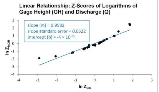
Numerous studies (e.g. Stuart and Emerman 2012) have shown that both gage height and discharge data are a better fit to a lognormal than a normal distribution. Therefore, the simplest rating curve is a linear relationship between the logarithm of gage height and the logarithm of discharge (see Fig. 2a). For each rating number at each gaging station, the gage height and discharge data were normalized by computing the Z-scores
Z!" !" =ln 𝐺𝐻 − ln 𝐺𝐻
Z!" ! =ln 𝑄 − ln 𝑄
𝜎!" ! (2)
where GH is gage height, Q is discharge, σ is standard deviation and an overbar indicates the mean. For rating numbers with negative gage heights (simply meaning lower than a fixed datum), a constant was added to all gage heights so that the smallest gage height became 0.001 feet. For each rating number, the normalized rating curve was then computed as the best-fit linear relationship
𝑍!" !" = 𝑚𝑍!" !+ 𝑏 (3)
where m and b are dimensionless slope and intercept, respectively (see Fig. 2b).
Figure 2a. The simplest rating curve is a linear relationship between the logarithms of gage height (GH) and discharge (Q). An example of a strong linear relationship (R2 = 0.92) is Rating No. 25 of the gaging station
on the Provo River at Provo, Utah (Site No. 10163000, USGS 2015a).
The next step was to determine whether there were clusters of dimensionless slopes (m) that would correspond to particular categories of rivers. Each linear relationship for a rating number was converted into a corresponding normal distribution with mean and standard deviation equal to the slope (m) and standard error of the slope (m), respectively (see Fig. 2c). The composite normal distribution for each gaging station had mean and standard deviation equal to the weighted mean of the slopes (m) of the rating numbers and the weighted mean of the standard errors of the slopes (m) of the rating numbers,
respectively. The weight for each rating number was based upon the number of data pairs in the rating number. The 191 gaging stations for which the weighted mean of the slopes was negative (m < 0) were discarded, now leaving 15,153 gaging stations. The composite normal distributions were then summed and divided by the remaining number of gaging stations to create a probability density function for dimensionless slopes (m) (see Fig. 3). The purpose of setting the width of the normal distribution of each rating number equal to
the uncertainty in slope was to keep poorly determined slopes from biasing the determination of peaks in the probability density function. The equivalent probability density function for intercepts (b) did not yield useful information, as the intercepts were negligible (see Fig. 2b), as would be expected for relationships between Z-scores.
Figure 2b. Rating curves were normalized by converting them into relationships between Z-scores. The example shown is Rating No. 25 of the Provo River at Provo, Utah (Site No. 10163000, USGS 2015a) (see Fig. 2a). The intercept of the linear relationship is negligible, as would be expected for relationships between Z-scores.
3. Results
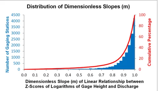
The normalized probability density function summed over for all gaging stations had only a single peak at m = 0.991 (see Fig. 3). Although the probability density function extended into the region m > 1, this was an artifact of the uncertainties in the slopes. There were no gaging stations with slope in the region m > 1, the largest slope being m =
0.999996 (see Fig. 4). The majority of gaging stations had slope close to but not exceeding
m = 1. The frequency of occurrence of slopes decreased dramatically with distance from m
= 1, but 30.1% of gaging stations were in the range 0 < m < 0.9 (see Fig. 4).
4. Discussion
The significance of the parameter m can now be understood by combining Eqs. (1)-(3) and setting b = 0 to yield
ln 𝐺𝐻 − ln 𝐺𝐻 = 𝑚𝜎!" !"
𝜎!" ! ln 𝑄 − ln 𝑄 . (4)
The slope of the ln GH vs. ln Q relationship is ∆ ln 𝐺𝐻
∆ ln 𝑄 = 𝑚 𝜎!" !"
Figure 2c. The linear relationships between the Z-scores of the logarithms of gage height and discharge were converted into normal distributions. The mean and standard deviation of the normal distribution is equal to the slope of the linear relationship and its standard error, respectively. The example shown is Rating No. 25 of the gaging station on the Provo River at Provo, Utah (Site No. 10163000, USGS 2015a) (see Figs. 2a-b). For gaging stations with multiple rating numbers, such as the example, the composite normal distribution has mean and standard deviation equal to the weighted mean slope and weighted mean standard error of all of the rating numbers, where the weighting is based upon the number of field measurements represented by each rating number.
Figure 3. The composite normal distributions for 15,153 gaging stations were summed and divided by the number of gaging stations. The normalized summation of the probability density functions had a single peak at m = 0.991, where m is the dimensionless slope of the linear relationship between Z-scores of logarithms of gage height and discharge (see Fig. 2b).
in which slope is now understood in terms of measured quantities, as opposed to the dimensionless slope (m) of the relationship between Z-scores. Now suppose that ln GH is
increased from its mean value to the limit of its range (e.g., three standard deviations) so that
∆ ln 𝐺𝐻 = 3𝜎!" !" (6)
If m = 1, then ln Q also increases to the limit of its range. In other words, there is a unique relationship between gage height and discharge, or gage height and discharge are
correlated. The majority of gaged rivers are close to this relationship between gage height and discharge (see Figs. 3-4).
Figure 4. Although the largest measured dimensionless slope (m) was m = 0.999996, there was no gaging station for which m ≥ 1. Over 30% of gaging stations had m < 0.9. The dimensionless slope (m) of the linear relationship between Z-scores of logarithms of gage height and discharge (see Fig. 2b) is a measure of the uniqueness of the gage height–discharge relationship. The case m > 1 indicates that discharge can vary without a variation in gage height. The case m = 1 indicates a unique relationship between gage height and discharge. The case m < 1 indicates that gage height can vary without a variation in discharge.
On the other hand, suppose that m > 1 and again that ln GH is increased from its mean value to the limit of its range. In that case, according to Eq. (5), ln Q cannot increase to the limit of its range. In other words, in this region, there can be variation in discharge that is not accompanied by variation in gage height. It is possible to imagine such a river that could, for example, accommodate a variation in discharge by digging out or filling in its channel without changing gage height. However, the results of this study have shown that such a gaged river does not exist (see Fig. 4). This observation does not appear to have been previously noted in the hydrologic literature, but justifies the conventional practice of plotting discharge as the independent variable (see Fig. 2a, USGS 2015a).
By the same reasoning, in the region 0 < m < 1, a variation in gage height can occur without an accompanying variation in discharge. All gaged rivers (neglecting those with a negative gage height-discharge relationship) are somewhere in this region (see Fig. 4), but for most rivers, the independence of gage height from discharge is small. However, for the over 30% of gaging stations in the region m < 0.9 (see Fig. 4), it could be argued that a rating curve is not an appropriate means of estimating discharge, as gage height can vary
independently from discharge. In summary, the parameter m is a measure of the
uniqueness of the gage height-discharge relationship, in which m = 1 indicates complete uniqueness or perfect correlation. The standard error of m (see Fig. 2b) is then a measure of confidence in the degree of uniqueness or correlation that is implied by the calculated value of m.
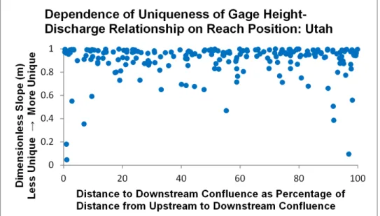
Based upon the objective of this research program, the next step was to ask what easily measurable characteristics are shared by rivers with low values of dimensionless slope (m). The question was focused on the 209 gaging stations in Utah with a useable history of simultaneous measurements of gage height and discharge, according to the criteria listed previously. Gaging stations with extreme variation in gage height without accompanying variation in discharge (m < 0.6) were found to occur close to either the nearest upstream confluence or downstream confluence (defined as 10% of the distance along the stream between the upstream and downstream confluences) (see Figs. 5a-b), where stream lengths and confluence positions were determined using the USGS National Hydrography Dataset (USGS 2015b). The primary sources of non-unique relationships between gage height and discharge are unstable channels, reverse flow from downstream tributaries, and unsteady flow, which could result either from tides or flood waves (Carter and Davidian 1968; Kennedy 1984; Kim et al. 2012). Avoiding sites close to either the upstream or downstream confluence (within 10% of the reach) precludes the effects of both flood waves from an upstream tributary and reverse flow from a downstream tributary. Although the importance of a station control, a natural or artificial feature that isolates a gaging station from downstream conditions, is emphasized in USGS manuals (Carter and
Davidian, 1968; Kennedy, 1984), we are not aware of previous quantitative guidelines for choice of sites for gaging stations.
Figure 5a. Based on the 209 gaging stations in Utah with a useable history of simultaneous measurements of gage height and discharge, gaging stations with extreme variation in gage height without accompanying variation in discharge (m < 0.6) occur close to either the nearest upstream confluence or downstream confluence. Distances were calculated from the National Hydrography Dataset (USGS 2015b).
Figure 5b. Based on the 209 gaging stations in Utah with a useable history of simultaneous measurements of gage height and discharge, extreme variation in gage height without accompanying variation in discharge (m < 0.6) can be avoided by not locating gaging stations close to either the nearest upstream or downstream confluence (defined as 10% of the distance along the stream between the nearest upstream and downstream confluences). Distances were calculated from the National Hydrography Dataset (USGS 2015b).
5. Conclusions
The first step in classifying rivers according to generic gage height-discharge rating curves has been to use only linear relationships, which classifies river sites into those with nearly unique gage height-discharge relationships and those for which rating curves are inappropriate because gage height can vary without a variation in discharge. An extension of the first step will be to consider a more exhaustive set of quantitative guidelines for choosing gaging station sites, such as the elevation differences between a gaging site and its upstream and downstream confluences, and the discharge at a gaging site as compared to the discharges of the upstream and downstream tributaries. Further steps will then involve considering increasingly more complex functional fits with the possibility of showing multiple peaks in the probability density function.
Acknowledgements. This research was a project of ENVT 4890 Surface Water Hydrology at Utah Valley University.
References
Bailey, J. F., 1966: Definition of stage-discharge relation in natural channels by step-backwater analysis.
U.S. Geological Survey Water-Supply Paper 1369-A, 24 p.
Birgand, F., G. Lellouche, and T. W. Appelboom, 2013: Measuring flow in non-ideal conditions for short term projects; uncertainties associated with the use of stage-discharge rating curves. Journal of
Hydrology, 503, 186-195.
Birkhead, A. L., and C. S. James, 1998: Synthesis of rating curves from local stage and remote discharge monitoring using nonlinear Muskingum routing. Journal of Hydrology, 205, 52-65.
Carter, R. W. and J. Davidian, 1968: General procedure for gaging streams. U.S. Geological Survey
Techniques of Water-Resources Investigations, Book 3, Chap. A6, 13 p.
Clarke, R. T., 1999: Uncertainty in the estimation of mean annual flood due to rating-curve indefinition.
Davidian, J., 1984: Computation of water-surface profiles in open channels. U.S. Geological Survey
Techniques of Water-Resources Investigations, Book 3, Chap. A15, 48 p.
DeGagne, M. P. J., C. G. Douglas, H. R. Hudson, and S. P. Simonovic, 1996: A decision support system for the analysis and use of stage-discharge rating curves. Journal of Hydrology, 184, 225-241.
Di Giammarco, P., M. Franchini, and P. Lamberti, 1998: The construction of the rating curve in river cross sections by using level data and a parametrized formulation of the Saint Venant equations. In 23rd
General Assembly of the European Geophysical Society: Hydrology, Oceans & Atmosphere.
Gauthier-Villars, p. 497.
Drus, S. A., 1982: Verification of step-backwater computations on ephemeral streams in northeastern Wyoming. U.S. Geological Survey Water-Supply Paper 2199, 12 p.
Dymond, J. R., and R. Christian, 1982: Accuracy of discharge determined from a rating curve. Hydrological
Sciences Journal, 27, 493-504.
Gergov, G., and T. Karagiozova, 2003: Unique discharge rating curve based on the morphology parameter Z. In Hydrology of Mediterranean and Semiarid Regions, E. Servat, W. Najem, C. Leduc, and A. Shakeel (eds.). IAHS-AISH Publication, 278, 3-8.
Jalbert, J., T. Mathevet, and A.-C. Favre, 2011: Temporal uncertainty estimation of discharges from rating curves using a variographic analysis. Journal of Hydrology, 397, 83-92.
Jarrett, R. D., and H. E. Malde, 1987: Paleodischarge of the late Pleistocene Bonneville Flood, Snake River, Idaho, computed from new evidence. Geological Society of America Bulletin, 99, 127-134.
Kean, J. W., 2004: Calculation of stage-discharge relations for gravel bedded channels. Journal of
Geophysical Research, 115, doi:10.1029/2009JF001398.
Kean, J. W., and J. D. Smith, 2005: Generation and verification of theoretical rating curves in the Whitewater River basin, Kansas. Journal of Geophysical Research, 110, doi:10.1029/2004JF000250. Kennedy, E. J, 1984: Discharge ratings at gaging stations. U.S. Geological Survey Techniques of
Water-Resources Investigations, Book 3, Chap. A10, 59 p.
Kim, D., S-K. Yang, and K. Yu, 2012. Analysis of loop-rating curve in a gravel and rock-bed mountain stream. Han’gug Sujaweon Haghoe Nonmunjib = Journal of Korea Water Resources Association, 45, 853-860.
Perumal, M., T. Moramarco, B. Sahoo, and S. Barbetta, 2007: A methodology for discharge estimation and rating curve development at ungauged river sites. Water Resources Research, 43,
doi:10.1029/2005WR004609.
Perumal, M., T. Moramarco, B. Sahoo, and S. Barbetta, 2010: On the practical applicability of the VPMS routing method for rating curve development at ungauged river sites. Water Resources Research, 46, doi:10.1029/2009WR008103.
Peterson-Overleir, A., 2004: Accounting for heteroscedasticity in rating curve estimates. Journal of
Hydrology, 292, 173-181.
Peterson-Overleir, A., 2005: Objective segmentation in compound rating curves. Journal of Hydrology, 311, 188-201.
Pickus, B., J. S. Herman, and A. L. Mills, 2014: Building rating curves for low-order streams draining small watersheds of the Atlantic Coastal Plain. Abstracts with Programs, Geological Society of America,
Southeastern Section, 46, 18.
Sahoo, G. B., and C. Ray, 2006: Flow forecasting for a Hawaii stream using rating curves and neural networks. Journal of Hydrology, 317, 63-80.
Sha, W., 2007: Flow forecasting for a Hawaii stream using rating curves and neural networks; discussion.
Journal of Hydrology, 340, 119-121.
Shao, Q., J. Lerat, G. Podger, and D. Dutta, 2014: Uncertainty estimation with bias correction for flow series based on rating curve. Journal of Hydrology, 510, 137-152.
Singh, V. J., H. Cui, and A. R. Byrd, 2014: Derivation of rating curve by the Tsallis entropy. Journal of
Hydrology, 513, 342-352.
Smith, C. F., J. T. Cordova, and S. M. Wiele, 2010: The continuous slope-area method for computing event hydrographs. Scientific Investigations Report, 2010, U. S. Geological Survey, 37 p.
Stuart, K. L., and S. H. Emerman, 2012: Developing rating curves for bedrock step-pool rivers using sparse data. In Proceedings of American Geophysical Union Hydrology Days 2012, J. Ramirez (ed.), 143-152. Available online at http://hydrologydays.colostate.edu/
Szilagyi, J., G. Balint, B. Gauzer, and P. Bartha, 2005: Flow routing with unknown rating curves using a state-space reservoir-cascade-type formulation. Journal of Hydrology, 311, 219-229.
USGS, 2015a: National Water Information System: Web Interface. Available online at
http://waterdata.usgs.gov/nwis
USGS, 2015b: Hydrography, National Hydrography Dataset, Watershed Boundary Dataset. Available online at http://nhd.usgs.gov/index.html
Weijs, S. V., R. Mutzner, and M. B. Parlange, 2013: Could electrical conductivity replace water level in rating curves for alpine streams? Water Resources Research, 49, 343-351.
Wilson, C. A. M. E., P. D. Bates, and J. M. Hervouet, 2002: Comparison of turbulence models for stage-discharge rating curve prediction in reach-scale compound channel flows using two-dimensional finite element methods. Journal of Hydrology, 257, 42-58.