Design and Construction of a Small Ammonia Heat Pump

Master of Science Thesis

KTH School of Industrial Engineering and Management Energy Technology EGI-2010-104

Division of Applied Thermodynamics and Refrigeration SE-100 44 STOCKHOLM

Design and Construction of a Small

Ammonia Heat Pump

Behzad Abolhassani Monfared

-2-

Master of Science Thesis EGI 2010:104

Design and Construction of a Small Ammonia Heat Pump

Behzad Abolhassani Monfared

Approved 2010-12-20 Examiner Björn Palm Supervisor Björn Palm

Commissioner Contact person

Abstract

In view of the fact that most of the synthetic refrigerants, in case of leakage or release, are harmful to the environment by contributing in global warming or depleting stratospheric ozone layer, many research works have been done recently to find alternative refrigerants posing no or negligible threat to the environment. Among alternative refrigerants, ammonia, a natural refrigerant with zero Global Warming Potential (GWP) and Ozone Depletion Potential (ODP), can be a sensible choice.

Although ammonia has been used for many years in large industrial systems, its application in small units is rare. In this project a small heat pump with about 7 kW heating capacity at -5 °C and +40 °C evaporation and condensation temperatures is designed and built to work with ammonia as refrigerant. The heat pump is expected to produce enough heat to keep a single-family house warm in Sweden and to provide tap hot water for the house. After successful completion of this project, it is planned to install the heat pump in a house to test it throughout a heating season to study its performance in real working conditions.

Since ammonia is flammable and toxic in high concentrations, the refrigerant charge is tried to be kept low in the heat pump to reduce the risk of fire or poisoning in case of unwanted release of refrigerant to the surroundings. The compact design of the heat pump helps reducing the refrigerant charge. Besides, considering the limited space normally reserved for installation of a heat pump in a house, the compact design of the heat pump is necessary.

-3-

Table of Contents

1.1.1 Environmental concerns in selection of refrigerant ... 7

1.1.2 Non-environmental criteria for selection of refrigerant ... 9

2 Objectives ...10

3 Method of attack ...11

4 Description of the test facility ...11

4.1 Main components of the heat pump...12

4.2 Main components of the heat source ...14

4.3 Main components of the heat sink ...15

4.4 Main electrical parts ...15

4.5 Measuring devices ...18

4.6 Control devices ...21

4.7 Data acquisition and processing ...22

5 Expected performance of the heat pump ...23

6 3-D drawing of the heat pump, heat source, and heat sink ...24

7 Construction of the test facility ...25

8 Heat pump performance calculations ...28

8.1 Evaporator ...28

8.2 Desuperheater and condenser ...29

8.3 Heating capacity, compressor work, and coefficient of performance ...32

9 Testing the heat pump ...33

10 Conclusions and suggestions ...35

Bibliography ...36

-4-

Table of Figures

Figure 1 Schematic drawing of the heat pump, heat sink, and heat source (tested in laboratory) ...12

Figure 2 Schematic drawing of the heat pump, heat sink, and heat source (installed in a house) ...12

Figure 3 The compressor of the heat pump, GOELDNER O 12 3 DK100...13

Figure 4 Pictures of the brass parts of the opened oil separator having been installed in an ammonia heat pump ...13

Figure 5 Coupled motor and compressor with rubber mountings ...15

Figure 6 Connection of main electrical parts ...17

Figure 7 Output signals from the energy meters (Brunata, 2006) ...19

Figure 8 Connection of the electrical resistor to take output signal and the capacitor to filter out the noise ...19

Figure 9 Schematic of measuring the power consumption of electrical heaters ...20

Figure 10 Wiring diagram for installation of power transducers ...20

Figure 11 A snap shot of the user interface of the Agilent VEE program ...23

Figure 12 a) An isometric view of the modeled geometry of the assembled components b) An isometric view of the frame on which the components are mounted...25

Figure 13 Cross section of 40mm×40mm aluminum bars used to make the frame ...26

Figure 14 (a) How the horizontal pipes are inclined upward in direction of the flow to avoid air lock (b) Air lock may occur in case of wrong inclination angel in the area indicated by a circle ...26

Figure 15 The completed test facility ...27

Figure 16 Key for the indices in Equations 8 and 9 ...28

Figure 17 Temperatures of the refrigerant and brine in the evaporator...29

Figure 18 Key for the indices in Equations 13 to 17 ...30

Figure 19 Temperatures of the refrigerant and water in the desuperheater ...31

Figure 20 Temperatures of the refrigerant and water in the condenser ...31

Figure 21 Key for the indices in Equation 27 ...32

-5-

Nomenclature

a constant in Equation 2

ATD approach temperature difference (K) b constant in Equation 2

COP1 coefficient of performance of heat pump cycle

cp heat capacity (kJ/kg-K)

Eelm electrical power consumption of the compressor’s motor (kW)

Ek compression work done on refrigerant (kW)

Epump electrical power consumption of brine pump in heat source loop (kW)

Etot sum of Eelm and Epump (kW)

hfg latent heat of vaporization (kJ/kg)

k1 constant in Equation 1

k2 constant in Equation 1

ke constant in Equation 2

ks constant in Equation 1

LMTD logarithmic mean temperature difference (K) mr mass flow rate of refrigerant (kg/s)

n rotation speed (rpm) P1 condensation pressure (bar)

P10 sensed pressure by the low-pressure side pressure transducer (bar)

P2 evaporation pressure (bar)

P35 sensed pressure by the high-pressure side pressure transducer (bar)

Pr ratio of P1 to P2

Q heat transfer rate (kW) Q1 heating capacity (kW)

Q2 cooling capacity (kW)

r ratio of Qdesup to Qcond

R2 _{coefficient of determination (of linear curve fitting)}

T temperature (°C)

t1 condensation temperature (°C)

t2 evaporation temperature (°C)

t2k intake temperature of compressor (°C)

U overall heat transfer coefficient (W/m2_-K)

UA product of overall heat transfer coefficient and effective area of heat exchanger (W/K) V volume flow rate (m3_/s)

-6- v specific volume (m3_/kg)

V10 output voltage signal from the low-pressure side pressure transducer (V)

V35 output voltage signal from the high-pressure side pressure transducer (V)

Vs swept volume (m3/s)

∆Psource pressure drop in heat source loop (bar)

∆T temperature difference (K) ∆TSC Subcooling (K)

∆TSH, ext external superheat (K)

∆TSH, int internal superheat (K)

ε effectiveness (of a heat exchanger) ηk isentropic efficiency

ηs volumetric efficiency

ηtot combined efficiency of inverter, electrical motor, and compressor

θi inlet temperature difference in heat exchanger (K)

θo outlet temperature difference in heat exchanger (K)

ρ density (kg/m3₎

Subscripts

cond condenser desup desuperheater DHW domestic hot water evap evaporator SH space heating

-7-

1

Introduction

Heat pump technology is widely used in Sweden with different applications; for example, only in district heating, approximately 9% of the supplied heat, around 4.5 TWh in 2008, was provided by heat pumps (Svensk Fjärrvärme, 2008). More than 800000 heat pumps were sold in Sweden between the years 1994 and 2008 (Forsén, 2009). This number is quite large compared to the number of heat pumps sold in other European countries, and also the share of small heat pumps installed in newly-built single-family houses is much larger than other types of heat pumps (WWF).

The heat pump designed and built in this project is also designed to be installed in a single-family house in Sweden to provide space heating and domestic hot water. Commercially-built heat pumps found in Swedish market with the same functionality usually have 5kW to 10 kW heating capacity, which typically covers about 90% of annual required heating and 60% of required heating power in the coldest days of the year. The heat is carried from 100m to 200m boreholes or ground surface soil to the evaporator of the heat pumps by the means of circulation of glycol or ethanol solutions at temperatures close to and below 0 °C. The heat is then transferred to the space heating system, having supply temperature of 35 °C to 50 °C or higher, and sanitary hot water, the temperature of which should exceed 60 °C periodically to thermally eliminate some microorganisms from water (Palm, 2008). The most common refrigerant for ground source heat pumps in Sweden is R407C. After R407C, R404A, R134a, and R290 are mostly used ones. For air-to-air heat pumps R410A is commonly used (Karlsson, et al., 2003).

In view of the fact that most of the synthetic refrigerants are harmful to the environment, many research projects have been carried out recently to use natural refrigerants such as ammonia (R717), but with reduced charge to avoid hazards in case of leakage (Granryd, et al., 2005). Besides, cost of preparation of natural refrigerants is much lower than that of HFCs (Hwang, et al., 1998).

1.1

Selection of refrigerant

Selection of a proper working fluid for the heat pump cycle, commonly referred to as refrigerant, is a decisive step in designing a heat pump. Some of the criteria for selection of the proper refrigerant are environmental concerns, performance of the heat pump in terms of capacity and efficiency, safety, price, compatibility with the materials and the compressor’s oil, and chemical stability (Kilicarslan, et al., 2005). 1.1.1 Environmental concerns in selection of refrigerant

In the early 1930s, chlorofluorocarbons (CFCs) and later on hydrochlorofluorocarbons (HCFCs) began to replace natural refrigerants such as ammonia and sulfur dioxide especially in domestic applications, due to their nonflammability and nontoxicity. However, as agreed in Montreal protocol in 1987 and Copenhagen amendments in 1992, use of CFCs and HCFCs is banned because of their high ozone depleting potential. The refrigerants used after phase out of CFCs and HCFCs are mostly chlorine-free refrigerants, such as R134a replacing R12, or mixtures of chlorine-free refrigerants, such as R407C replacing R22. Although chlorine-free molecules such as hydrofluorocarbons (HFCs) do not effectively participate in the depletion of the stratospheric ozone layer, many of them have high global warming potential (Granryd, et al., 2005); accordingly, their usage has been limited by Kyoto Protocol in 1997 along with other greenhouse gases (United Nations, 1998).

A refrigerant may participate in global warming directly, due to its molecular structure when it is released to the atmosphere, or indirectly, considering the energy needed for preparation of the refrigerant and efficiency and energy consumption of the cycle, in which the refrigerant is used. The indirect effect of a refrigerant, related to the energy consumption, has a significant share in total equivalent warming impact; it is, however, not easy to determine since it depends on many local factors such as the efficiency of the cycle, generation method of the consumed electricity, and refrigerant production processes (Calm, 2006). 1.1.1.1 Direct impact of selected refrigerant on global warming

An advantage of ammonia as an alternative for the synthetic refrigerants is that the emission of ammonia into the atmosphere, unlike almost all other refrigerants, is harmless to the environment in terms of its

-8-

global warming potential and ozone depletion potential, which are both zero. Besides, it is biodegradable with atmospheric lifetime of few days (ASHRAE, 2002).

In a comparison between 40 refrigerants to rank them based on their global warming potential (GWP, relative to CO2 based on 100-year time horizon), ozone depleting potential (ODP, relative to R11), and

atmospheric lifetime (ALT, number of years), Restrepo, et al. (2008) have found only R1270 (propene, GWPR1270=3, ODPR1270=0, ALTR1270=0.001) and R601 (n-pentane, GWPR601=0, ODPR601=0, ALTR601=

0.01) less harmful than R717 (ammonia, GWPR717=0, ODPR717=0, ALTR717=0.25) to the environment due

to their shorter atmospheric lifetime. However, Calm and Hourahan (2001) have mentioned much higher GWP values for R1270 and R601, which are about 20 and 11 respectively based on 100-year time horizon, and atmospheric lifetime of ammonia is considered only few days in a position document approved by ASHRAE in 2002 and 2006 (ASHRAE, 2002).

1.1.1.2 Indirect impact of selected refrigerant on global warming Although ammonia is considered a natural refrigerant since its molecules are found in nature, the ammonia used as refrigerant is produced through industrial processes, which may contribute to global warming (Hwang, et al., 1998). Campbell and McCulloch (1998) have estimated the equivalent amount of produced CO2, assumed to be entirely released to the environment, per kilogram of manufactured

ammonia, 2 kgCO2/kg, and have compared to that of R134a, 6 to 9 kgCO2/kg, R22, 3 kgCO2/kg, R12, 3

kgCO2/kg, Isobutane, 0.5 kgCO2/kg, and cyclopentane, 1 kgCO2/kg. However, energy consumption

and CO2 release in production process of refrigerants are insignificant compared to the consumed energy

and equivalent CO2 emissions during the lifetime of a heat pump or refrigeration cycle. (Campbell, et al.,

1998). Therefore, performance of the cycle which depends on the design of the cycle with regard to the working condition and thermodynamic and transport properties of the refrigerant, besides its GWP, is a decisive factor determining the total equivalent warming impact of a system.

Coefficient of performance of a vapor compression cycle may not vary dramatically by changing the working fluid, which meets the pressure and temperature requirements of an application, while the working conditions are kept similar. Hence, properties of the selected refrigerant cannot guarantee the efficient performance of a system (Dossat, 1991), and consequently, reduction in energy consumption and indirect participation on global warming. However, coefficient of performance of heat pump cycle (COP1)

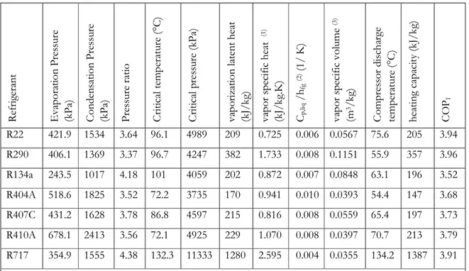
of a cycle, with different refrigerants, modeled in Engineering Equation Solver (EES) software program (Klein, 2009) with evaporation temperature of -5 °C, condensation temperature of 40 °C, superheating of 5K, subcooling of 5K, and assumed electrical motor efficiency of 80% is estimated and tabulated in Table 1. The refrigerants in this modeling are ammonia, currently used refrigerants in domestic heat pumps in Sweden, which are R407C, R404A, R134a, R290, and R410A, and, for comparison, R22. In the model no pressure drop or heat transfer with ambient is taken into account, and volumetric efficiencies and isentropic efficiencies are estimated using equations of general form of Equation 1 and Equation 2, where ηs is volumetric efficiency; ηk is isentropic efficiency; a, b, k1, k2, ks, and ke are constants; t2k (°C) is intake

temperature of compressor; P1 is condensation pressure; P2 is evaporation pressure; t1 (°C) is

condensation temperature; t2 (°C) is evaporation temperature (Granryd, et al., 2005).

η_s=k1.൬1+ks. t2k-18 100 ൰ .e k2.P_P1 2 Equation 1 η_s η_k=൬1+ke. t2k-18 100 ൰ .e (ୟ ୲భ + 273.15 ୲మାଶ଻ଷ.ଵହା ୠ) Equation 2

-9-

Table 1 Comparison between few refrigerants in a modeled cycle with evaporation temperature of -5 °C, condensation temperature of 40 °C, superheating of 5K, subcooling of 5K, and assumed electrical motor efficiency of 80%. (Pressure losses and heat transfer to ambient is neglected) (Engineering Equation Solver, Klein 2009)

R ef ri ge ra n t E va p o ra ti o n P re ss u re (k P a) C o n d en sa ti o n P re ss ur e (k P a) P re ss u re r at io C ri ti ca l te m p er at ur e (° C ) C ri ti ca l p re ss u re ( kP a) v ap o ri za ti o n la te n t h ea t (k J/ k g) v ap o r sp ec if ic h ea t (1 ) (k J/ k g. K ) Cp ,li q / hfg (2 ) (1 / K ) v ap o r sp ec if ic v o lu m e (3 ) (m 3/ kg ) C o m p re ss o r d is ch ar ge te m p er at u re ( °C ) h ea ti n g ca p ac it y (k J/ k g) C O P1 R22 421.9 1534 3.64 96.1 4989 209 0.725 0.006 0.0567 75.6 205 3.94 R290 406.1 1369 3.37 96.7 4247 382 1.733 0.008 0.1151 55.9 357 3.96 R134a 243.5 1017 4.18 101 4059 202 0.872 0.007 0.0848 63.1 196 3.52 R404A 518.6 1825 3.52 72.2 3735 170 0.941 0.010 0.0393 54.4 147 3.68 R407C 431.2 1628 3.78 86.8 4597 215 0.816 0.008 0.0559 65.4 197 3.73 R410A 678.1 2413 3.56 72.1 4925 229 1.070 0.008 0.0397 70.7 213 3.79 R717 354.9 1555 4.38 132.3 11333 1280 2.595 0.004 0.0355 134.2 1387 3.91

(1) saturated vapor at evaporation temperature

(2) ratio of specific heat of saturated liquid at condensation temperature to latent heat of vaporization at evaporation temperature

(3) superheated vapor at compressor inlet

Calculated COP1 values in Table 1 for R717 (ammonia), R290 (Propane), and R22 are almost the same

and higher than that of the rest of the refrigerants for the assumed working condition, which may be taken as an indicative of more efficient performance. However, the estimated values should be interpreted with care as some assumptions and simplifications have been made in modeling. For example, if pressure drops were introduced to the model, the COP1 of ammonia cycle might become more than the others since less

pressure losses are expected in ammonia cycle due to its low molecular weight (Lorentzen, 1988). Another point to be considered in interpreting the COP1 values in Table 1 is that the rather low

temperature of the discharged refrigerant vapor from compressor is not enough for producing sanitary hot water except for ammonia cycle. It implies that, to produce sanitary hot water, higher condensation pressure is needed for the refrigerants other than ammonia which leads to lower COP1 values for them

than the tabulated ones.

1.1.2 Non-environmental criteria for selection of refrigerant

In general, some transport and thermodynamic properties of a refrigerant are more important to have more desirable operation of a heat pump. It is desirable for a refrigerant to have evaporation pressure higher than atmospheric pressure to prevent inward air and moisture leakage. Too high condensation pressure necessitates heavy pipes and fittings which increases the costs. Large latent heat of vaporization and also low specific volume of vapor of a refrigerant result in less required mass flow rate of refrigerant, less required compressor displacement, and less power consumption. Refrigerants with high thermal conductivity need smaller heat exchangers, as they have higher heat transfer coefficient. If liquid suction heat exchanger is used, low heat capacity of liquid and high heat capacity of vapor are desirable to have enough subcooling and not excessive superheating. In addition, low heat capacity of liquid, by increasing the subcooling effect, increases the heating capacity per unit mass flow rate of heat pump (Dossat, 1991)

-10-

on the grounds that the needed amount of refrigerant vaporizing in the expansion device to cool down the liquid decreases if the heat capacity of liquid is low (Pita, 1984); that is, after expansion valve more liquid is remained, which increases the cooling capacity for a given mass flow rate of refrigerant. Small specific heat compared with latent heat of vaporization reduces the losses in the expansion process. Smaller pressure ratio results in higher volumetric efficiency of compressor; hence, it reduces the compressor work and increases the COP of the system. In addition, to have low pressure drop, low viscosity of refrigerant is desirable (Granryd, et al., 2005).

Ammonia, as a refrigerant, has favorable properties. Its low molecular weight, 17.03 kg/kmol, results in high vaporization latent heat, low pressure drop, desirable heat transfer properties, and less losses in throttling. With high vaporization latent heat of the refrigerant smaller pipes and fittings can be used (Lorentzen, 1988). Because of the high vaporization latent heat and low vapor specific volume of ammonia, the highest and the lowest in Table 1, smaller displacement of compressor and mass flow rate are needed; therefore, with smaller compressor, less energy is needed to run the cycle. Furthermore, its small specific heat compared with latent heat of vaporization, the smallest in Table 1, reduces the losses in the expansion process. Besides, it has low cost and is not sensitive to water contamination (Dincer, 2003). Ammonia, in spite of its favorable properties and advantages, has some drawbacks, limiting its application. It is flammable in the range of concentration of 16% to 25% by volume in air, but it is hard to ignite and does not sustain the flame in absence of the flame source. In addition to flammability, the products or the released heat of its reaction with acids or halogens may pose some dangers (Dincer, 2003). Ammonia is also toxic. Its odor can be smelt at 5ppm or greater concentration; it irritates eye at 100 ppm to 200 ppm; nevertheless, no permanent eye damage is caused in concentrations lower than 500 ppm. At 400 ppm it irritates throat and cause cough at 1700 ppm. More than 30 minutes exposure to ammonia with concentration of 2400 ppm or higher is lethal. The maximum concentration at which one can be exposed to ammonia for 30 minutes without health damage is 500 ppm. Contact with liquid ammonia can burn skin. The pungent odor of ammonia even in low concentrations may cause panic, which can lead to problems more serious than the ones related to flammability or health risk; the odor, however, is an effective warning to alarm the people in case of release or leakage (ASHRAE, 2002). Another drawback of ammonia is that it is corrosive to copper, zinc, and their alloys in presence of water (Lorentzen, 1988). Furthermore, most of the commonly used oils, lubricating compressor, are immiscible in ammonia; it may make the oil-return to the compressor problematic; nevertheless, since ammonia is lighter than oil, the oil can be drained and taken back to the compressor. High temperature of discharge gas after compressor may also result in decomposition of oil (Granryd, et al., 2005). However, in this project, the high discharge temperature is used as an advantage to produce hot water.

2

Objectives

In this project a small ammonia heat pump, with reduced charge to reduce the fire and poisoning risk in case of leakage, providing about 7 kW heat, sufficient for space heating and tap water heating of a small typical Swedish single-family house, is designed. The specifications of its components are determined based on the required functionality of the heat pump at its expected working conditions. The heat pump and its accompanying devices such as expansion tank and pump for heat source brine circuit, some parts of heat sink water circuit, electrical parts, measurement devices, and control units and actuators are designed to fit into a 60 by 60 square centimeters space, which is the dimension of commercially-built heat pumps for domestic applications.

The designed heat pump is intended to have satisfactory performance with ammonia as refrigerant, the amount of which is kept low due to flammability and toxicity of ammonia in high concentrations.

After doing necessary calculations and developing a geometric model of the test facility, the heat pump is built with designed components and is tested afterwards.

-11-

3

Method of attack

Using Engineering Equation Solver (EES) (Klein, 2009) software program, a simplified model of the heat pump is developed to estimate the performance of the heat pump and to predict the working parameters, used in sizing different components and pipes. Besides, older thesis reports and experiences gained in previous ammonia heat pump projects are used. In order to simulate the real working conditions of a heat pump, installed in a single-family house with bedrock as heat source, a brine circuit with electrical heaters is used as heat source, and a water circuit serves as heat sink.

A scaled three-dimensional model is drawn to design the heat pump and the other components, which are normally placed in the same package in commercially-built heat pumps, compact enough to fit into a 60 by 60 square centimeters space. Compactness of the heat pump also helps to reduce the refrigerant charge. The designed heat pump is built in Applied Thermodynamics and Refrigeration Laboratory, Department of Energy Technology, Royal Institute of Technology (KTH), Sweden. The constructed heat pump is used to perform experiments.

4

Description of the test facility

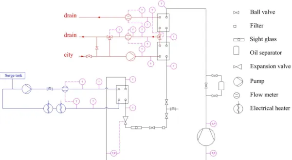
The ammonia vapor leaving the compressor is cooled in a separate heat exchanger called desuperheater in order that the heat from gas cooling is utilized for heating domestic hot water. The heat taken from condensation in the condenser is to be used in hydronic space heating system; however, in the experiments performed in laboratory the heat is transferred from the desuperheater and the condenser to a water circuit serving as heat sink. The subcooled refrigerant leaving the condenser is expanded in an electronic expansion valve keeping the superheat in desired range. The two-phase fluid coming from the expansion valve is heated in the evaporator to enter the compressor as super heated gas. The transferred heat in the evaporator comes from either electrical heaters, in laboratory experiments, or bedrock borehole. A schematic drawing of the heat pump, heat source, and heat sink can be seen in Figure 1 and Figure 2. Figure 1 shows the configuration used for laboratory experiments. The heat pump installed in a house looks schematically like Figure 2.

The water leaving the condenser is expected to be around 40°C, which is almost the design condensation temperature of the heat pump. The water temperature after the desuperheater is to be 60°C. Temperature of water after condenser and desuperheater can be regulated by setting the position of 3-way valves and the speed of pump.

In the heat source loop, the water temperature varies with the evaporation temperature, speed of the pump, and the amount of heat taken from the electrical heaters or borehole.

-12-

Figure 1 Schematic drawing of the heat pump, heat sink, and heat source (tested in laboratory)

Figure 2 Schematic drawing of the heat pump, heat sink, and heat source (installed in a house)

In the following parts main components and devices installed in the test facility are introduced. A complete list of the parts and components is available in Appendix A.

4.1

Main components of the heat pump

An open-type reciprocating HKT-GOELDNER compressor, O 12 3 DK100, is used to run the heat pump. The expected cooling capacity of the heat pump for condensation temperature of 40°C and evaporation temperature of -5 to 0°C, when the rotation speed is 1450 rpm, is about 6 kW according to the data provided by the manufacturer of the compressor, HKT Huber-Kälte-Technik GmbH (HKT-Goeldner, 2007). More detailed specification of the compressor is available in Appendix B. The oil in the

-13-

compressor is drained and is replaced by oil miscible in ammonia, FUCHS RENISO GL 68. Figure 3 is a picture of the compressor.

Figure 3 The compressor of the heat pump, GOELDNER O 12 3 DK100

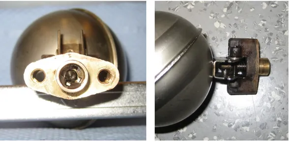
The oil separator installed in the heat pump, Danfoss OUB1, is designed for CFCs, HCFCs, and HFCs (Danfoss, 2005), and the oil return outlet at the bottom of the separator is made of brass. Nonetheless, after opening a similar oil separator which had been installed in an ammonia heat pump for about 3 years, it has been observed that the brass parts are not corroded. Figure 4 shows pictures of the brass parts of the previously used oil separator.

-14-

The desuperheater and the condenser, ALFANOVA27-10H and ALFANOVA52-20H plate heat exchangers, Alfa Laval products, are entirely made of stainless steel (Alfa Laval, 2010). Effective heat transfer surface area of the desuperheater and the condenser are 0.2 m2 _{and 0.918 m}2 _{(Alfa Laval AB,}

2009).

The expansion device used in this heat pump is a Carel electronic expansion valve, E2V09BS000. Although the chosen expansion valve is not corroded by ammonia, it has not been specifically designed for ammonia heat pumps. Nevertheless, the size of the expansion valve has been chosen by relying on the experience gained in previous projects (Sarmad, et al., 2007).

The evaporator is a minichannel aluminum heat exchanger. As reported by Sarmad, D. et al (2007), the heat exchanger is expected to reduce the refrigerant charge with still satisfactory heat transfer performance. The mean effective heat transfer surface area of the evaporator is 0.8 m2 _{(Fernando, 2007).}

All of the pipes, connections, and valves in contact with ammonia are stainless steel. In this project, the main criterion of sizing the steel pipes is the minimum flow velocity needed to return the oil to compressor. However, unnecessarily narrow pipes are avoided to prevent high pressure drop.

As a rule of thumb, the suggested flow velocity in suction and discharge line is between 5 and 10 m/s and in liquid line is 0.7 to 1.5 m/s to ensure the oil return to the compressor (Granryd, 2005). Considering the insolubility of most of the commonly used oils in ammonia, pipes are chosen conservatively. The pipes selected for different parts are listed in Table 2.

Table 2 Selected sizes of the pipes of the heat pump

Pipe size (mm) Anticipated pressure drop per unit length (kPa/m)

Discharge line 12×1 2.04

Desuperheater to condenser 10×1 4.51

Condenser to expansion valve 6×1 2.94

Expansion valve to evaporator 6×1 2.94

Suction line 12×1 5.20

A stainless steel liquid filter, a Swagelok product, is installed after the condenser to remove the impurities floating in the refrigerant. The manually operated valves in contact with ammonia are also made of stainless steel. In order to check whether any refrigerant vapor is passing through the expansion valve, a cylindrical sight glass is placed after the filter.

4.2

Main components of the heat source

A high efficiency variable speed Grundfos pump, CME3-3 A-R-A-E AVBE, is used to circulate the brine, ethanol 25% wt, through the evaporator and the electrical heaters in laboratory experiments or, alternatively, bedrock borehole, when installed in a house. The pump is sized to circulate ethanol 25% wt through a U-shaped 40×2.4 high density polyethylene borehole heat exchanger placed in a 200-meter borehole with Reynolds number of 3500, corresponding to the flow of 3.03 m3_{/hr at -5°C. The rest of}

pressure drops are assumed to be equivalent to 40 m extra length of borehole heat exchanger. Finally the pump is sized for 3.03 m3_{/hr flow and 22 m-brine pressure drop. The other criteria to choose the pump}

are the efficiency of the pump, supplied power frequency, geometrical dimensions, suitability for the application, compatibility of the shaft seal material with the brine, and the possibility of stepless speed control through external 0-10 DC Voltage. Performance curves of the pump and its electrical motor are available in Appendix D.

-15-

The electrical heaters, replacing bedrock borehole when the experiments are performed in laboratory, consist of three 1500 W heaters and three 1000 W heaters. A transformer controls one of the 1000 W heaters and the rest of the heaters are on-off controlled, so the input power to the heat source circuit can be adjusted in the range of 0 to 7500 W.

Since the heat source circuit, either with electrical heaters or bedrock borehole heat exchangers, is a closed loop, an 8-liter expansion tank, Grundfos GT-H-8 PN10 G 3/4 V, is added to provide room for expanded fluid in the heat source loop. However, the expected change in the volume of the brine is much less than 8 liters.

4.3

Main components of the heat sink

A high efficiency variable speed pump, WILO Stratos ECO 25/1-5 BMS, is used to circulate water through the desuperheater, the condenser, and the rest of the heat sink circuit. The pressure drop in desuperheater and condenser is estimated to be 0.6 m-H2O for 0.77 m3/hr flow, which is estimated based on the expected water temperature change in condenser. Nevertheless, the pump is sized for 1.2 m-H2O pressure drop to take the rest of the pressure drops into account and have a safety margin. The other criteria to choose the pump are the efficiency of the pump, supplied power frequency, geometrical dimensions, suitability for the application, and the possibility of stepless speed control through external 0-10 DC Voltage.

Two 3-way valves, SIEMENS VXG41.1401 and SIEMENS VXG41.1301, automatically-driven by SIEMENS Acvatix SKD62 actuators and Eurotherm 2408 PID controllers, are used to regulate the amount of water passing through the desuperheater and the amount of drained water. Positions of the 3-way valves are determined based on the sensed temperature of water after condenser and after desuperheater.

4.4

Main electrical parts

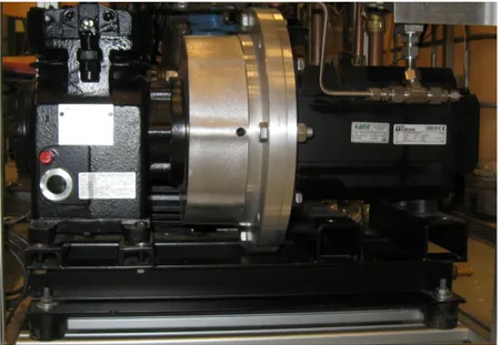
The compressor, O 12 3 DK100, is coupled with an efficient 6-pole electrical motor with permanent magnets, TG drives TGT6-2200-20-560/T1P (see Figure 5). The rotation speed of the motor is controlled by the means of a frequency inverter, OMRON V1000 45P5, used together with a 3-phase filter, Rasmi A1000-FIV 3030-RE. The output frequency of the inverter is set by 0-10 DC voltage signal; alternatively, it can be set manually through operator keypad. The electricity coming to the filter, and thereupon to the inverter and motor, can be cut off by the means of a 3-phase switch. An on-off switch is also used to operate the crankcase heater of the compressor.

-16-

For each single-phase pump, used in heat sink and heat source loops, in addition to 0-10V control signal, an on-off switch is installed.

Three 1.5kW and two of 1kW electrical heating elements, serving as heat source in laboratory, are turned on or off by switches. The input power to another 1kW electrical heating element is controlled by a variable transformer.

A transformer, TUFVASSONS PVS 120A, with 120VA output power and 24VAC output voltage, is used to supply power for the actuators of the 3-way valves and the driver of the expansion valve.

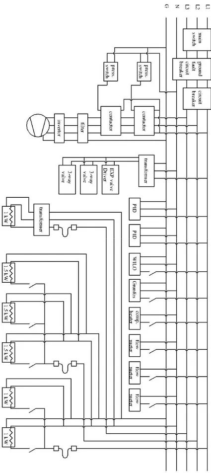
Flow meters, power meters, PID controllers, pressure controllers, data acquisition units, and a computer are connected to one of the live lines and the neutral line. It has been tried to have rather balanced load on lines of supplied three-phase power. There is also a main switch to cut off the electricity from the whole system. Figure 6 shows how the electrical parts are connected. The electrical heaters are only used in the laboratory set-up.

-17-

-18-

4.5

Measuring devices

Two energy meters, Brunata HGQ1-R0-184/1B0R24, are installed to estimate the rate of heat transfer in desuperheater and condenser. Another energy meter, Brunata HGS5-R0-184/1B0R24, is also added to the brine side to estimate the cooling capacity of the heat pump. Energy meters measure volumetric flow rate and temperatures before and after the heat exchangers and calculate the rate of heat transfer between the heat exchangers and the refrigerant, provided that the heat exchangers are insulated effectively to eliminate the effect of heat transfer from the ambient air. The energy meters have a built-in database for water by which they calculate the enthalpy change of water flow based on the volumetric flow rate and the two sensed temperatures according to Equation 3.

Q (kW)= V(m3_{/s) . ∆T(K) . (ρ . cp) (kJ/m}3_{-K) Equation 3}

Q is the amount of transferred heat to or from the fluid flow; V is volume flow rate; ∆T is the temperature change of the fluid; ρ is the density of the fluid; cp is heat capacity of the fluid.

The fluid in heat source loop is ethanol 25% wt instead of water. Although the ρ.cp value of ethanol 25%

wt is different from water, its value is close to that of water. For example, at 0°C, ρ.cp is 4146 kJ/m3-K for

ethanol 25% wt and is 4227 kJ/m3_{-K for water. Accordingly, a water energy meter is used for brine side;}

however, the read value of the cooling capacity is to be corrected for ethanol 25% wt.

The energy meters have been selected based on the anticipated flow rate going through the flow sensor of the energy meter.

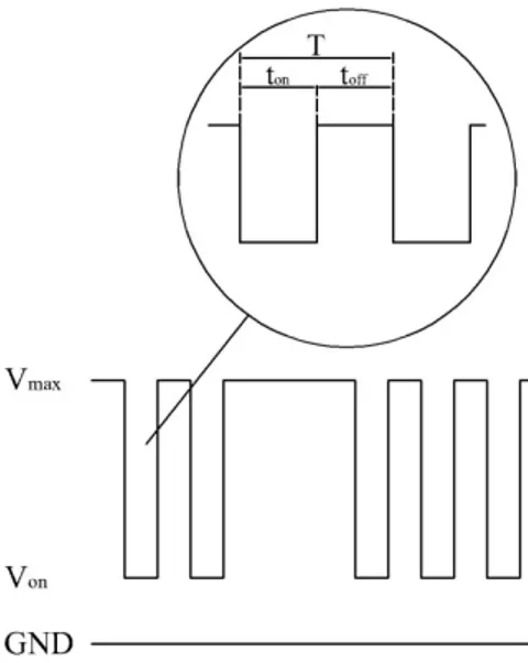
In addition to reading from the display of the energy meters, the measured flow rate or energy rate can be read by counting the output pulses of the energy meters over a time period. Each pulse is representative of an amount of liquid, depending on how the energy meters are programmed, passed through the flow meter’s sensor. The output pulse is of the form shown in Figure 7. The voltage of the sent signal, Von,

which is about 1.5 Volts, is lower than the voltage when there is no pulse. The maximum voltage varies between 5V and 28V, about 6.1V in the current set-up, depending on the electrical resistor used, the resistance of which is about 0.92 kΩ in the current set-up. Figure 8 shows how the electrical resistor is connected. The minimum possible pulse period, T= ton + toff, for which the flow meters are currently

programmed, is 40ms; however, flow meters may be programmed for larger pulse periods with increment of 40ms. The programmed pulse period is chosen with regard to the maximum flow to be measured. The pulse period and the maximum flow to be measured determine the volume per pulse value, for which the energy meter needs to be programmed (Brunata, 2006).

In the current set-up, the output pulses for volumetric flow rate are used to log the data automatically. To filter out the noises a capacitor is installed in parallel with output pulse source of each energy meter. Then Equation 3, with different ρ.cp values for water and ethanol solution, is used to calculate the cooling and

-19-

Figure 7 Output signals from the energy meters (Brunata, 2006)

Figure 8 Connection of the electrical resistor to take output signal and the capacitor to filter out the noise

To have an estimation of the amount of the heat that will be removed from bedrock boreholes and also to check the cooling capacity measured by energy meter, the electricity consumption of the electrical heaters in the laboratory set-up is measured. For measuring the power consumption of the heaters, as shown schematically in Figure 9, the voltage between the neutral line and the live line is measured, and the current is measured indirectly through measuring the voltage drop, in millivolts, along a low resistance resistor. Each 6 mV voltage difference over the resistor corresponds with the current of 1 A. The power consumption can be calculated by multiplying the directly measured voltage and the indirectly measured current.

Figure 9 Schematic of measuring the power consumption

The power consumption of compressor and the pump on the brine loop is measured by the means of two active power transducers, Eurotherm E1

phase unbalanced load of 1 to 3.125 kW

(Eurotherm, 2001). The output 4-20mA signal from the power transducers is log through a Data Acquisition/Switch Unit, Agilent 34970A.

power transducers.

a) EuroTherm E1-3W4

Figure 10 Wiring diagram for installation of power transducers

The temperature sensors of the energy meters are Pt500 resistance thermometers; the temperature probe used to control the expansion valve is

thermocouples. All of the thermocouples have reference junctions, the temperatures of which are determined by a four-wired Pt100 resistance thermometer. For pressure measurements piezoresistive pressure transducers are used.

The signals from pressure transducers, thermocouples, energy meters, and power transducers are acquired by a Data Acquisition/Switch Units, Agilent 34970A. To record the measurements and process them, the measured values are sent to an Agilent VEE program

The pressure transducers are calibrated by a MARTEL/BETA calibrator, which consists of a pneumatic pump, MECP500, and a gauge, 321A. The voltage signals from the pressure transd

-20-

Schematic of measuring the power consumption of electrical heaters

The power consumption of compressor and the pump on the brine loop is measured by the means of two herm E1-3W4 and Eurotherm E1-1W0. The former one measures 3 1 to 3.125 kW, and the latter one measures single-phase load up to 1

20mA signal from the power transducers is logged

through a Data Acquisition/Switch Unit, Agilent 34970A. Figure 10 is a diagram of the wiring of the

b) Eurotherm E1-1W0 Wiring diagram for installation of power transducers

The temperature sensors of the energy meters are Pt500 resistance thermometers; the temperature probe used to control the expansion valve is a thermistor, and the rest of temperature sensors are T type thermocouples. All of the thermocouples have reference junctions, the temperatures of which are

wired Pt100 resistance thermometer. For pressure measurements piezoresistive

The signals from pressure transducers, thermocouples, energy meters, and power transducers are acquired by a Data Acquisition/Switch Units, Agilent 34970A. To record the measurements and process them, the measured values are sent to an Agilent VEE program (Agilent Technologies, 2010) installed on a PC. The pressure transducers are calibrated by a MARTEL/BETA calibrator, which consists of a pneumatic pump, MECP500, and a gauge, 321A. The voltage signals from the pressure transducer on low

The power consumption of compressor and the pump on the brine loop is measured by the means of two 1W0. The former one measures

3-phase load up to 1953 W by a computer is a diagram of the wiring of the

The temperature sensors of the energy meters are Pt500 resistance thermometers; the temperature probe the rest of temperature sensors are T type thermocouples. All of the thermocouples have reference junctions, the temperatures of which are wired Pt100 resistance thermometer. For pressure measurements piezoresistive

The signals from pressure transducers, thermocouples, energy meters, and power transducers are acquired by a Data Acquisition/Switch Units, Agilent 34970A. To record the measurements and process them, the

installed on a PC. The pressure transducers are calibrated by a MARTEL/BETA calibrator, which consists of a pneumatic

-21-

side, ClimaCheck PA-22S/10bar/780935.13, measuring the gauge pressure between 0 and 10 bars, are read by the data acquisition unit for 2.000 bars, 3.550 bars, 5.500 bars, and 9.000 bars of absolute pressure. For each pressure level the average of several readings are calculated. Then the pressure and output voltage correlation, Equation 4, is found by using linear curve fitting. The voltage signals from the pressure transducer on high-pressure side, ClimaCheck PA-22S/35bar/780935.13, measuring the gauge pressure between 0 and 35 bars, are read by the data acquisition unit for 3.000 bars, 8.500 bars, 10.000 bars, 13.500 bars, 15.550 bars, and 19.500 bars of absolute pressure. For each pressure level the average of several readings are calculated. Then the pressure and output voltage correlation, Equation 5, is found by using linear curve fitting. The output voltage signal from both of the pressure transducers is in the 1 to 5 V range, and the atmospheric pressure at the time of calibration was 1.015 bar. The coefficient of determination, R2_{, of the fitted lines, Equation 4 and Equation 5, is 1.00.}

P10 (bar, abs)= 2.504V10 (V) – 1.524 Equation 4

P35 (bar, abs)= 8.745V35 (V) – 7.794 Equation 5

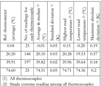
To calibrate the thermocouples, the averaged values of readings of the data acquisition unit from thermocouples in a period are compared with the average of the readings of a calibrated Pt100, Pentronic 21-4300250, class DIN 1/3 according to IEC 60 751, as reference in the same period. The measurements of the Pt100 are read by the means of a handheld instrument, Dostmann P650 with accuracy of ±0.03 °C and resolution of 0.01 K between -100 °C and 150°C (Dostmann electronic, 2005). For this purpose, the thermocouples and the reference thermometer are placed in a liquid bath at 0 °C, 20 °C, 40 °C, and 75 °C, the temperature of which is kept constant by ISOTECH HYPERION calibrating equipment. It is observed that the largest difference between the averaged values of readings of each thermocouple and the average of readings of reference thermometer in the same period is less than 0.2 K; some other statistical details are listed in Table 3.

Table 3 Details of verifying the readings of thermocouples

R ef . t h er m o m et er (a v er ag e) ( °C ) N o . o f re ad in gs f o r ea ch t h er m o co u p le A v er ag e & m ed ia n (1 ) (° C ) S ta n d ar d d ev ia ti o n (1 ) (K ) H ig h es t re ad te m p er at u re (2 ) ( °C ) L o w es t re ad te m p er at u re (2 ) ( °C ) M ax im u m a b so lu te d ev ia ti o n (2 ) ( K ) 0.04 25 -0.01 0.03 0.15 -0.20 0.19 20.20 148 20.10 0.03 20.28 19.53 0.57 39.91 197 39.82 0.02 39.96 39.64 0.18 74.60 25 74.51 0.05 74.71 74.36 0.2 (1) All thermocouples

(2) Single extreme reading among all thermocouples

The readings of thermocouples are not corrected on the grounds that larger errors, with unknown values, are introduced to the temperature measurements due to the placement and installation of thermocouples (Peter Hill, personal communication, August 27th_{, 2010).}

4.6

Control devices

To control the rotation speed of the motor driving the compressor and pumps, DC voltage signals are sent to the devices as output of the data acquisition units. The magnitude of the output DC voltage signals are determined by the user of the Agilent VEE software program.

-22-

For superheat control, the position of the expansion valve is determined by a standalone driver, EVD0000E50, which controls the superheat based on the received signals from a pressure transducer and a resistance thermometer installed before the intake of the compressor. The driver, alternatively, can work as a positioner controlled externally by an input signal.

The actuators of the 3-way valves, SIEMENS Acvatix SKD62, are controlled by two PID controller devices, Eurotherm 2408. Each PID controller measures the input signal from the thermocouple connected to it and sends 0-10 DC output voltage signal to the actuator of the 3-way valve. The valve installed between desuperheater and condenser makes more flow pass through the desuperheater when the temperature after desuperheater gets higher than 60 °C. The other 3-way valve circulates less water when the temperature after condenser is more than 40 °C.

To protect the compressor and other components from too low suction pressure or too high discharge pressure, two pressure switches, Danfoss RT 1A and RT 6AW, compatible with ammonia, has been selected with regard to the expected working pressure ranges. The low-pressure pressure switch is set on 1.4 bar (gage) to avoid evaporation temperatures below -15 °C to make sure that the brine does not freeze. The high-pressure pressure switch is set on 20 bar (gage) to protect the desuperheater and condenser from pressures higher than their maximum allowable working pressure.

4.7

Data acquisition and processing

Signals from thermocouples and pressure transducers are acquired and converted to temperature and pressure readings in Agilent 34970A, Data Acquisition/Switch Units. The signals from power transducers, pulse train from the energy meters, and voltage measurement signals are also acquired by the Data Acquisition/Switch Unit. Depending on the type of inserted plug-in modules and the way it is programmed, the data acquisition unit can read temperature, AC/DC voltage, electrical resistance, frequency, period, number of pulses, AC/DC current, and digital 8-bit or 16-bit words ; it can also send digital output 8-bit or 16-bit words and analog output DC voltage. The data acquisition unit, besides, has some options, although limited, to process the read values. Programming the data acquisition unit can be done manually through the front panel of the device or remotely through a PC. In this project, to have the readings recorded and to have more control and processing options, the data acquisition unit is set up and run by a software program written in Agilent VEE programming language.

The written Agilent VEE program assigns the channels of the acquisition unit to measure different quantities and configures the measurement parameters. Then, after asking for the interval between each set of readings and the magnitude of output DC voltages, it starts the readings with the indicated time interval in between. Based on the measurements, the Agilent VEE program calculates the cooling capacity, electricity consumption of the electrical heaters, heat for space heating, heat for domestic hot water, heat transferred in the condenser, heat transferred in the desuperheater, and COP1. The data acquired after each set of readings and calculated values are stored in an MS Excel file, a text file, and an array of records, called DataSet in Agilent VEE programming language, which is saved as a text file. Simultaneously the changes of parameters of interest with time, from the beginning of the test, are shown in graphs. While the program is running, the time interval between series of readings and the output DC voltage signals can be actively changed by the user, to control the rotational speed of electrical motors of the pumps and compressor. The recorded data in an MS Excel file or a text file is used for further processing and analysis.

-23-

Figure 11 A snap shot of the user interface of the Agilent VEE program

5

Expected performance of the heat pump

To predict the performance of the heat pump, a simple software model by the means of EES has been developed. In addition to the design values of evaporation temperature and condensation temperature, which are respectively -5°C and 40°C, both the superheating and subcooling has been assumed to be 5K. In addition, the cooling capacity of the heat pump has been assumed to be 5.41 kW based on the information given by the producer of the compressor (HKT-Goeldner, 2007). The volumetric efficiency and isentropic efficiency of the compressor can be estimated by applying Equation 6 and Equation 7, which are Equation 1 and Equation 2 with constants suggested for ammonia (Granryd, et al., 2005). However, the volumetric efficiency given by Equation 6 results in too high swept volume rate not corresponding with the data provided by the manufacturer of the compressor (see Appendix B); therefore, it is decided to use volumetric efficiency of 71.6% based on the data provided by the manufacturer of the compressor to find isentropic efficiency from Equation 7.

Equation 6 ηs is volumetric efficiency; Pr is the ratio of P1, condensation pressure,to P2, evaporation pressure; 1.02

and -0.063 are constants given by Granryd, E. et al. (2005) for ammonia.

η_ୱ

η_୩= exp ൤−1,69 ൬

tଵ+ 273,15

tଶ+ 273,15൰ + 1,97൨

Equation 7

ηs is volumetric efficiency; ηk is isentropic efficiency; -1.69 and 1.79 are constants given by Granryd, E. et

al. (2005) for ammonia.

For the given values the EES software model predicts refrigerant’s mass flow rate of mr = 0.0049 kg/s,

heating capacity of Q1= 6.92 kW, and swept volume of Vs= 0.0024 m3/s= 8.75 m3/hr. Shares of

condenser and desuperheater from the heating capacity are anticipated to be Qcond= 5.51 kW and Qdesup=

1.40 kW respectively. The compression work done on the refrigerant is estimated Ek= 1.51 kW, so the

-24-

ratio of heating capacity to compression work is calculated 4.6. The set of equations used for the EES model and the detailed calculation results are available in Appendix C.

6

3-D drawing of the heat pump, heat source, and heat

sink

To have a plan to place all of the components, except the electrical heaters, in a block with 60×60 cm2

cross section and acceptable height, which are the dimensions of a typical commercially-built domestic heat pump, and also to design the heat pump compactly to reduce the amount of charge, the geometry of the components are modeled in a scaled 3-D drawing, created in AutoCAD®. The 3-D model helps to have a general overview of the test facility before its construction, so the limited space can be used efficiently.

The drawing is made with enough details to provide an intuitive and easy to understand picture of the real heat pump. Figure 12a shows an isometric view of the drawing. 3-D drawings of the pumps are taken from the Web sites of GRUNDFOS and WILO companies (Grundfos, 2010) (WILO, 2010). The frame, on which the heavy components are mounted, is shown separately in Figure 12b.

-25-

(a) (b)

Figure 12 a) An isometric view of the modeled geometry of the assembled components b) An isometric view of the frame on which the components are mounted

7

Construction of the test facility

The frame on which the heavy components are mounted is made up of 40mm×40mm aluminum bars produced by AluFlex®. The cross section of the aluminum bars can be seen in Figure 13.

-26-

Figure 13 Cross section of 40mm×40mm aluminum bars used to make the frame

The placement of the mechanical components is based on the 3-D drawing, a view of which is shown in Figure 12a, and heavy components are fixed to the frame. As it can be seen in Figure 5, to reduce noise and vibration, rubber mountings are used for the coupled compressor and motor. The same type of mountings is also used for the brine pump installed in heat source loop.

The measuring devices except power transducers are installed on pipelines between the mechanical components according to Figure 1. The thermocouples and the thermistor connected to the expansion valve driver are placed in temperature wells, filled with thermal grease, while the Pt500 thermometers are in direct contact with liquid. It is tried to install the thermometers perpendicular to or preferably in opposite direction of flow.

On the hot water side or brine side, it has been tried to fix the horizontal pipes with slight upward inclination in the direction of the flow, as shown schematically in Figure 14a, to ensure that air lock is prevented because of wrong inclination angel of the pipes, shown in Figure 14b. In addition, bleed valves have been used in topmost part of pipelines for bleeding the pipes of the trapped air.

(a) (b)

Figure 14 (a) How the horizontal pipes are inclined upward in direction of the flow to avoid air lock (b) Air lock may occur in case of wrong inclination angel in the area indicated by a circle

After completion of piping the water side and brine side are filled with pressurized water to make sure the pipes and heat exchangers do not leak. Then the refrigerant side is pressurized with nitrogen and leaking spots is detected by soap and water solution. To decide whether the refrigerant side is leak-free, it, pressurized with nitrogen, is left for few days to see whether pressure divided by absolute temperature

-27-

remains constant. Furthermore, when the system is filled with refrigerant, wet litmus paper is used to recheck the refrigerant side for leakage.

The next step after tightening the leaking connections is insulation of the pipes, heat exchangers, oil separator, and electrical heaters. The used insulating material, ARMAFLEX, product of ArmaCell, is 1 cm or 2 cm thick, depending on the surface temperature and geometry.

For safety reasons, plastic electrical boxes are installed above the heat pump in a space separated from the water and brine circuits by a metal sheet. Figure 6, schematically, shows how the electrical parts are installed. Figure 15 is a picture of the completed test facility.

-28-

8

Heat pump performance calculations

8.1

Evaporator

The measured volumetric flow rate and temperatures of brine before and after evaporator give the cooling capacity according to Equation 8. The density and heat capacity used in Equation 8 are those of ethanol 25% wt solution at inlet temperature to the evaporator and average temperature of the brine passing through evaporator, respectively. The indices in Equation 8 are taken from Figure 16. The properties of the brine can be read from Table 4. The calculated heat is sum of the heat coming from boreholes (electrical heaters in laboratory experiments) and the pump work, if the heat transfer to the ambient is insignificant.

Figure 16 Key for the indices in Equations 8 and 9

Qevap (kW)= V8(m3/s).ρ8(kg/m3).cp(kJ/kg-K).(T8-T7)(K) Equation 8

Table 4 Density and heat capacity of ethanol 25% wt between -10 °C and +10 °C (Melinder, 2007)

Temperature (°C) Density (kg/m3) Heat capacity (kJ/kg-K)

+10 967.0 4.280

0 971.0 4.270

-10 974.5 4.260

On refrigerant side Equation 9 can be written. The measured evaporating pressure and temperature after the evaporator give the enthalpy after evaporator, h12, and enthalpy before evaporator, h6, can be taken

equal to the enthalpy after the condenser, h5 in Figure 16, assuming isenthalpic throttling process in the

expansion valve takes place. Enthalpy after condenser, h5, is determined by the measured condensing

pressure and temperature after the condenser. Mass flow rate of refrigerant, mr, can be found from

Equations 8 and 9.

Qevap (kW)= mr(kg/s).(h12 – h6)(kJ/kg) Equation 9

Figure 17 shows temperature changes of the refrigerant and the brine in evaporator. With reference to Figure 17, the Logarithmic Mean Temperature Difference (LMTD) can be calculated by using Equation 10, if the pressure drop and superheat in the evaporator is neglected. The Approach Temperature Difference (ATD) in evaporator is equal to θo in Figure 17. If Qevap and LMTDevap are calculated,

-29-

area, for evaporator (Granryd, et al., 2005). Effectiveness of the evaporator is found from Equation 12 (Incropera, et al., 2002).

Figure 17 Temperatures of the refrigerant and brine in the evaporator

LMTDevap (K)= (θi - θo)(K)/Ln(θi /θo) Equation 10

Qevap (kW)= (0.001)(kW/W).UAevap(W/K).LMTDevap(K) Equation 11

εevap= (T8 – T7)/(T8 – T6) Equation 12

8.2

Desuperheater and condenser

The flow meter installed after condenser measures the volumetric flow rate of a part of the water passing through the condenser; the rest of the water leaving the condenser goes through the desuperheater and is measured with the other flow meter. That is, the sum of measurements of the two flow meters in heat sink circuit is the total amount of water heated in the condenser. Accordingly, if the measured flow rates in the flow meters after condenser and after desuperheater are respectively named V10 and V11, heat

transfer in desuperheater, Qdesup, and heat transfer in condenser, Qcond, can be calculated by using

Equations 13 and 14. The indices are based on Figure 18.

Qdesup (kW)= V11(m3/s).ρ11(kg/m3).cp(kJ/kg-K).(T11-T10)(K) Equation 13

-30-

Figure 18 Key for the indices in Equations 13 to 17

To find mass flow rate of refrigerant, mr, Equation 15 can be used. The measured condensing pressure

and temperatures before desuperheater and after condenser give the enthalpies h3 and h5. Although

Equations 16 and 17 are also correct, they cannot directly give the mass flow rate of refrigerant, since the phase of the refrigerant and, therefore, the enthalpy between desuperheater and condenser cannot be determined by the measured condensing pressure and the temperature of the refrigerant at that point. On the other hand, if the mass flow rate of refrigerant is known from Equation 9 or Equation 15, the state of the refrigerant between the two heat exchangers can be determined by Equation 16 or 17.

(Qdesup + Qcond) (kW)= mr(kg/s).(h3 – h5)(kJ/kg) Equation 15

Qdesup (kW)= mr(kg/s).(h3 – h4)(kJ/kg) Equation 16

Qcond (kW)= mr(kg/s).(h4 – h5)(kJ/kg) Equation 17

Figure 19 shows temperature changes of the refrigerant and water in desuperheater. With reference to Figure 19, the Logarithmic Mean Temperature Difference (LMTD) can be calculated by using Equation 18. If Qdesup and LMTDdesup are calculated, Equation 19 gives UA-value, product of overall heat transfer

coefficient and effective heat transfer surface area, for desuperheater. Effectiveness of the desuperheater is found from Equation 20 (Incropera, et al., 2002).

-31-

Figure 19 Temperatures of the refrigerant and water in the desuperheater

LMTDdesup (K)= (θi - θo)(K)/Ln(θi /θo) Equation 18

Qdesup (kW)= (0.001)(kW/W).UAdesup(W/K).LMTDdesup(K) Equation 19

εdesup= (T3 – T4)/(T3 – T10) Equation 20

Figure 20 shows temperature changes of the refrigerant and water in condenser. With reference to Figure 20, the Logarithmic Mean Temperature Difference (LMTD) can be calculated by using Equation 21, if the pressure drop, desuperheating, and subcooling in the condenser is neglected. The Approach Temperature Difference (ATD) in condenser is equal to θo in Figure 20. If Qcond and LMTDcond are calculated, Equation

22 gives UA-value, product of overall heat transfer coefficient and effective heat transfer surface area, for condenser (Granryd, et al., 2005). Effectiveness of the condenser is found from Equation 23 if the desuperheating from T4 to t1, condensation temperature, is negligibly small. To be more accurate the

numerator of the left-hand side of Equation 23 should be reduced proportional to the desuperheating from T4 to t1.

Figure 20 Temperatures of the refrigerant and water in the condenser

LMTDcond (K)= (θi - θo)(K)/Ln(θi /θo) Equation 21

Qcond (kW)= (0.001)(kW/W).UAcond(W/K).LMTDcond(K) Equation 22

-32-

8.3

Heating capacity, compressor work, and coefficient of

performance

Heating capacity (Equation 24) is the sum of rate of heat transfer in desuperheater and condenser or sum of the heat used for space heating and providing domestic hot water.

Q1 (kW)= Qdesup(kW) + Qcond(kW) = QDHW(kW) + QSH(kW) Equation 24

Neglecting the consumption of the pump circulating water in heat sink circuit and that of other measurement and control devices, the total electricity consumption (Equation 25) is sum of the consumptions of the brine pump in heat source loop and that of the motor of the compressor, including losses of inverter.

Etot (kW)= Epump(kW) + Eelm(kW) Equation 25

Coefficient of performance, COP1, can be calculated by dividing heating capacity by total electrical power

consumption (Equation 26).

COP1= Q1(kW)/Etot(kW) Equation 26

Provided the mass flow rate of refrigerant, mr, is found from heat balance over heat exchangers according

to Equations 9 or 15, the compression work done by the compressor on the refrigerant is given by Equation 27. Indices 1 and 2, according to Figure 21, are for suction line and discharge line.

Figure 21 Key for the indices in Equation 27

Ek(kW)= mr(kg/s).(h2 – h1)(kJ/kg) Equation 27

If volumetric efficiency, ηs, swept volume flow, Vs, and specific volume at compressor intake, v1, are

known, Equation 28 gives the mass flow rate of refrigerant.

mr(kg/s)= ηs.Vs(m3/s)/v1(m3/kg) Equation 28

Using Equation 29, ηtot, covering losses in compressor, electric motor, and inverter which are transferred

to the ambient as heat, can be calculated.

Ek(kW)= Eelm(kW) . ηtot Equation 29

The overall energy balance of the heat pump yields Equation 30, provided that the heat transfer to the ambient is insignificant.

-33-

9

Testing the heat pump

After constructing the test facility, the heat pump has been run to detect and fix possible problems. The measurements recorded by the Agilent VEE program for a steady operation of the test facility, with compressor shaft rotation speed of 1500 rpm, is shown in Figure 22 and Table 5. The exchanged heat rates and COP1, calculated as explained in section “8 Heat pump performance calculations”, can also be

read from Figure 22 or Table 5.

Using Equation 9 and Equation 15, mass flow rate of refrigerant is calculated 0.0049 kg/s and 0.0051 kg/s, the difference of which is 4%. For evaporation and condensation temperatures of -5.4 °C and 40.0 °C the volumetric efficiency can be approximated 71.2% based on the data provided by the manufacturer of the compressor (see Appendix A). The swept volume at rotation speed of 1500 rpm is about 9.36 m3_{/hr, so the mass flow rate of refrigerant, using Equation 28, can be estimated at 0.0052 kg/s, 6% and}

2% higher than the values given by Equation 9 and Equation 15. The mass flow rate included in Table 5 is average of the values given by Equation 9 and Equation 15, because the value given by Equation 28 is based on estimation of volumetric efficiency not on measurements.

Figure 22 Steady operation of the test facility (the compressor’s motor is running at 1500 rpm, 75 Hz)

The isentropic efficiency of the compressor, ηk, is calculated 82.2%, which is 10.3% higher than the value

predicted by EES model described in section “5 Expected performance of the heat pump”, 71.9%. If the average of the mass flow rate values given by Equation 9 and Equation 15 is used, the volumetric efficiency of the compressor, from Equation 28, is found 69.3%, which is slightly less than the value estimated based on the data given by the manufacturer of the compressor, 71.2%. Considering the significance of the effect of pressure ratio on isentropic and volumetric efficiencies, it worth mentioning that the evaporation and condensation pressures, and therefore the pressure ratio Pr= 4.45, are very close

to the design conditions used in the predicting EES model and the conditions at which the compressor manufacturer has evaluated the performance of the compressor.

The compression work done on the refrigerant, the cooling capacity, and the heating capacity are calculated 1.38 kW, 5.44 kW, and 7.03 kW. By dividing compression work by the electrical power consumption of the compressor ηtot, covering the losses in the inverter, electrical motor, and compressor,

-34-

If the overall energy balance of the heat pump is investigated according to Equation 30, the right-hand side is 0.21 kW more than the left-hand side. This difference can be the result of combination of the effect of the errors in measurements and unexpected inward flow of energy to the system. The temperatures in Figure 22 suggest that heat can only be transferred from the ambient to the evaporator, the line between expansion valve and evaporator, and the line between the evaporator and the compressor because in the rest of the areas the temperatures are above the ambient temperature. However, the evaporator and the line between the expansion valve and the evaporator are insulated well. There is poor insulation only over the line going to the compressor because of the limited space; nevertheless, the heat transfer to the system through that line from the ambient, which causes external superheat of 2.3 K, is only 0.032 kW. Therefore, the error in the overall energy balance is mostly due to measurement errors.

Compared with the results of the EES model presented in section “5 Expected performance of the heat pump” the ratio of heating capacity to compression work done on the refrigerant, 5.1, is higher than the predicted value, 4.6. The reason for higher Q1/Ek can be the higher isentropic efficiency of the

compressor than expected value, which results in lower discharge temperature and enthalpy, and therefore lower compression work. However, as mentioned before, there is a 0.21 kW error in energy balance, which can be the reason of the differences between the obtained results and predicted ones.

Table 5 Steady operation of the test facility (indices for temperatures and flow rates are in accordance with Figure 22)

T1 (°C) -1.5 Pr 4.45 ηtot (%) 75.6 T2 (°C) 127.5 t1 (°C) 40.0 COP1 3.2 T3 (°C) 126.6 t2 (°C) -5.2 LMTDdesup(K) 13.7 T4 (1) (°C) 40.3 V8 (m3/hr) 1.636 LMTDcond (K) 1.95 T5 (°C) 33.5 V10 (m3/hr) 0.626 LMTDevap (K) 6.43 T6 (°C) -5.2 V11 (m3/hr) 0.054 UAdesup (W/K) 90.43 T7 (°C) -0.3 Qdesup (kW) 1.242 UAcond (W/K) 2972 T8 (°C) 2.6 Qcond (kW) 5.788 UAevap (W/K) 845.7 T9 (°C) 32.4 Q1 (kW) 7.03 U desup(3) (W/m2_-K) 452.2 T10 (°C) 39.8 Q2 (kW) 5.437 U cond (3) (W/m2_-K) 3237 T11 (°C) 59.9 Eelm (kW) 1.827 Uevap (3) (W/m2_-K) 1057

T12 (°C) -3.8 Epump (kW) 0.359 ATDcond (K) 0.17

∆TSC (K) 6.5 Ek (kW) 1.38 ATDevap (K) 5.1

∆TSH, int (K) 1.4 mr (2) (kg/s) 0.005 εdesup 0.994

∆TSH, ext (K) 2.3 Vs (m3/s) 0.0026 εcond 0.936

P1 (bar) 15.5 ηk (%) 82.2 εevap 0.375

P2 (bar) 3.5 ηs (%) 69.3 ∆Psource (bar) 1.24

(1) Corrected for enthalpy and pressure at point 4

(2) Average of the values given by Equation 9 and Equation 15 (3) Assumed to be constant all over the heat exchanger