MÄLARDALEN UNIVERSITY
SCHOOL OF INNOVATION, DESIGN AND ENGINEERING
VÄSTERÅS, SWEDEN
Thesis for the Degree of Bachelor in Computer Science 15 hp
GRAPH GENERATION ALGORITHMS
FOR THE GRADE DECISION CANVAS
William Achrenius
was15001@
student.mdh.se
Martin Bergman Törnkvist
mtt15001@
student.mdh.se
Examiner
:Federico Ciccozzi
Mälardalen University, Västerås, Sweden
Supervisor: Antonio Cicchetti
Mälardalen University, Västerås, Sweden
28 September 2018
William Achrenius Graph Generation Algorithms Martin Bergman Törnkvist for the Grade Decision Canvas
Abstract
Development in the field of software architecture, from the early days in the mid-80’s, has been significant. From purely technical descriptions to decision based architectural knowledge, software architecture has seen fundamental changes to its methodologies and techniques. Architectural knowledge is a resource that is managed and stored by companies, this resource is valuable because it can be reused and analysed to improve future development. Companies today are interested in the reasoning behind the software architecture. This reasoning is mainly formulated through the architectural decisions made during development. For architectural decisions to be easier to analyse they need to be stored in a way that enables use of common analytical tools so that comparisons between decisions are consistent and relevant. Additionally, it is also important to have enough data, which leads us to the problem that, preferably, all the individual architectural knowledge cases must be structured and stored. To do this we present a tool that uses graph generation algorithms to generate architectural knowledge as graphs based on an architectural decision canvas called GRADE. This enables multiple decision cases to be encoded through graphs that can be used to analyse relationships and balances between different architectural knowledge elements represented through nodes and edges within a graph.
William Achrenius Graph Generation Algorithms Martin Bergman Törnkvist for the Grade Decision Canvas
Table of Contents
1. Introduction
5
2. Background
6
2.1 GRADE Taxonomy 6
2.2 The Graph Data Model 7
2.3 Model and Metadata Repository 8
2.4 Motivations behind Architectural Decision Models 8
3. Related Work
10
3.1 Artificial Data Systems 10
3.2 Graph Generation 10
4. Problem Formulation
12
5. Method
13
6. Ethical and Societal Considerations
14
7. Generating Decision Cases
15
7.1 Illustrated Input and Output 15
7.2 Using Excel Files to Store the Primitive Data 15
7.3 Random Generation 16
7.4 Algorithm Process Overview 16
7.5 Pseudocode 17
8. Results
19
8.1 Number of Nodes and Relationships 19
8.1.1 Minimum and Maximum Number of Nodes and Relationships 20
8.2 Properties and Relationships 21
8.3 Decision Case from the Manually Created Data Repository 23
9. Discussion
25
10. Conclusions
26
11. Future Work
27
12. References
28
Appendices
30
Appendix A 30 Appendix B 32 3William Achrenius Graph Generation Algorithms Martin Bergman Törnkvist for the Grade Decision Canvas
List of Figures
1. Figure 1: Example of nodes and relationships in a Neo4j database. 8 2. Figure 2: Input and Output visualisation of the decision case creation process. 15 3. Figure 3: Row 1 to 6, pseudocode of the algorithm. 17 4. Figure 4: Row 7 to 18, pseudocode of the algorithm. 17 5. Figure 5: Row 19 to 31, pseudocode of the algorithm. 18 6. Figure 6: Row 32 to 38, pseudocode of the algorithm. 18 7. Figure 7: Artificially generated decision case. 21 8. Figure 8: Decision case from the manual data repository. 23 9. Figure 9: Excel file containing metadata of node categories. 30 10. Figure 10: Complete pseudocode of the algorithm. 32
List of Tables
1. Table 1: Number of nodes and relationships generated by the algorithm. 19 2. Table 2: Number of nodes and relationships found in the manual data repository. 20 3. Table 3: Minimum and maximum number of nodes and relationships possible to generate. 21 4. Table 4: Name and number of relationships generated by the algorithm for a decision case. 22 5. Table 5: Name and number of relationships from a decision case in the manual repository. 24
William Achrenius Graph Generation Algorithms Martin Bergman Törnkvist for the Grade Decision Canvas
1.
Introduction
Development in the field of software architecture, from the early days in the mid-80’s, has been significant. Early concepts and methodologies for industrial architectural development produced purely technical
architectural knowledge that described the system in terms of system structure and behaviour. As the software industry evolved the methods of describing system architecture were faced with a paradigm shift. The new methods involved stakeholders and were more interested in the how and why a certain architecture produced the documented result. This is referred to as architectural decision management and provided methods for
facilitating and organising architectural knowledge. Architectural decision management contrasted against the earlier methods were software architects would use their experience and previous knowledge to make the architectural decisions [1].
To account for the change, in the dynamics of architectural decisions, the decisions evolved into, more commonly, group decisions. The involvement of stakeholders impacted the decision-making process. To continue to make good decisions, consensus between different stakeholders and developers became an important issue. If a stakeholder’s point of view on a decision is undervalued in the architectural decision-making process, the final software product might not be accepted by that stakeholder [2]. This is the core of architectural design, where the skills and knowledge of all individuals are brought together [3]. Philippe Kruchten [4] suggests that architectural design decisions are the most important aspect of developing software-intensive systems. He continues to mention that software architecture also encompasses attributes such as usage, functionality and performance. In the process of presenting and storing the architecture, using graphics and other tools, we lose some of the architectural knowledge, the rationale behind the decisions.
Different companies store and use their architectural knowledge in different ways. As architectural
decision-making includes early interaction with stakeholders, this provides advantages in early assessment of the architectures quality attributes. Considerable progress has been made in this area. Despite this, representing, capturing and maintaining knowledge about software architectures remains a challenge due to a lack of methods and techniques. The key components of architectural knowledge contain the design decisions and their rationale. However, companies tend to use different words that have the same meaning, for example, some authors might term design decisions and mean architectural decisions [5].
GRADE [6] is an architectural decision canvas that attributes to efficient adaptation and evolution of software architectures. This enables for large-scale complex systems to have more flexible architectures for future maintenance. The canvas encompasses software’s architectural knowledge in a structured fashion and improves access to decisions made. This access opens for discussions between decision makers and supports the process of decision-making by highlighting important elements that describe the decisions.
Companies architectural decisions can often be closely related and through GRADE these decisions can be standardised and analysed on a detailed level. This allows for a deeper understanding of the relations and provides the ability to analyse through comparison of decisions made.
To analyse the properties of architectural decisions there needs to be enough data. Comparing decisions from many different companies require a common data repository, and an effective way of generating that data, that can be used to represent the GRADE canvas. The way we capture, represent and maintain can, in this way, be enhanced. Using GRADE model as a template for data repositories, all the interconnected parts of the decisions made can be analysed more effectively through a common medium. This report will present a way to
accomplish this.
William Achrenius Graph Generation Algorithms Martin Bergman Törnkvist for the Grade Decision Canvas
2.
Background
2.1 GRADE Taxonomy
GRADE is a decision canvas created to capture architectural decisions during software and systems
development [6]. The decision canvas is created to provide a way to capture architectural decisions and collect data [7], it’s also meant to provide a way to discuss around the decisions made and the data collected. The idea is to establish a method that can be used to capture architectural decisions.
The taxonomy is created to be able to support development in three main ways [7]. Firstly, by structuring decisions it helps to identify new opportunities in the development. Secondly it supports the review of alternative options within the development to help make informed decisions around all available options. Thirdly it supports the evaluation of a decision by describing the decision, what factors might influence it and what the outcome might be.
The canvas has five main categories that are used to describe decisions, each of these higher-level categories then contains several more specific topics that relates to the category [7], more information about each element and category can be found in another paper by Papatheocharous et al. [8]. The main categories, that have been identified in the GRADE taxonomy and are used to create the decision cases can be found in [7] and [8], they are the following:
Goals: Describes the main goal of the decision, valuable targets that have been identified and are important when stakeholders must make architectural decisions. The goals can be described from several different perspectives that affect the decision case in different ways. Depending on the perspective, different goals can be identified. Some examples:
● Customer: To improve the quality of the product and allow it to have extended functionality. ● Financial: Increase the company profits.
● Internal business: To extend to new markets and increase the internal competence within the company. ● External production: To save costs on the development and to reduce debt.
● Innovation and learning: To enter an ecosystem, create new partners or evolve current partnerships and increase sales.
Roles: Describes which stakeholders are involved in the decision. The roles can be anyone from the owner of
the product to the users of supporters. Anyone that can have an impact on what decisions are made can be in this category. There can be many different roles affecting a specific decision case, some roles such as Asset supplier, Asset user and System End-User might not be directly involved in the decision-making but are still important roles such that their involvement in the decision case can still affect the decision-making. Other roles such as Initiator, Supporter, Influencer and Decider can be more directly involved in the decision-making process and directly influence the outcome of the development.
Assets: Describes different alternatives or options of assets that exist. Assets have several key attributes which
help to characterize them. The origin describes where the asset comes from and are developed. Examples of origin assets are reusable source code or open source code that can be used in the development.
An asset can in addition have a Usage perspective that describes the development option for the asset, examples:
● Reuse: An asset that is reused.
● Buy: An asset that is bought and used.
● Develop: An asset that is developed by the company.
William Achrenius Graph Generation Algorithms Martin Bergman Törnkvist for the Grade Decision Canvas
The type describes what the asset type is, examples of asset types are Information Asset, Software Asset, System Asset, Hardware Asset or Service Asset. These assets could for example be a database or server.
The properties describe the assets most important properties, both functional and non-functional properties. These are some examples of topics that can be non-functional properties:
● Reliability ● Performance ● Operability ● Security ● Compatibility ● Maintainability ● Transferability ● Economy
Decision methods and criteria: Describes what methods have been used to make the decision and what set of
criteria or properties that was used. This category uses two main elements to support the decision, the criteria and the method family. The criteria element has its own categories to help determine the criteria, the categories are:
● Functionality: The capability of the product to provide the stated functions.
● Quality: States the non-functional qualities.
● Time to market: The time it will take for the product to hit the market.
● Financial: Different financial criteria that relate to the development of the product.
● Risk: Possibilities and risks of unforeseeable or important events that can cause losses to the company. In turn, the method family has its own set of categories that can be used, examples:
● Expert-based: Judgement that is provided and based on expertise in the area.
● Memory-based (Analogy): Using data from previous or similar projects as the basis for estimating costs, risks etc.
● Parametric: A technique to calculate estimates for costs, budgets, durations, etc.
● Non-parametric: A method used in statistics that analyses data with small sample sizes.
Environment: Describes the context of the decision case so it’s possible to understand it. The environment category is the most external one in comparison to the other categories, since it’s possible for it to describe circumstances that are out of control of the decision maker. Some examples of the main perspectives for the environment category are the following:
● Organization: Information about the company to put it in a context, for example information about the structure or distribution within the company.
● Product: Contextual information related to the product or service being provided.
● Stakeholder (non-decision): Stakeholders that might have influence on the decision or might be
affected by the decision but are not having any part in the decision-making process directly.
● Market and Business: Contextual information about the current market. Customers, competitors, partners, etc.
2.2 The Graph Data Model
Graph database data is modelled in graph data structures. Using graph structures bring several advantages when working with graph data. One advantage is the fact that manipulations of the structures is accomplished by using graph-oriented operations [9]. Operations such as finding shortest path or finding different subgraphs within the structure allows the user to query the database on a high abstraction level.
William Achrenius Graph Generation Algorithms Martin Bergman Törnkvist for the Grade Decision Canvas
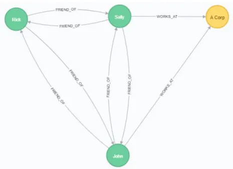
Another advantage is that the model is more visual to the user and therefore allows for a more natural handling of the data. The model can display data in similar ways that we might think about it. It can store all information about an entity in a single node and then draw the relations between different nodes to model the relationships between entities. Figure 1 displays how nodes and relationships can be visualized in a graph database. The example is created in Neo4j, the current most popular database according to DB-engines ranking [10].
Figure 1: The people and the corporation are displayed as nodes with different colours in the database. Their arrows point between the nodes to display the relationships between them.
2.3 Model and Metadata Repository
A repository is a central accessible component that stores information about artefacts [11]. The artefacts can be anything from source code or documents to special purpose models such as data models for defining
relationships. The main difference between a repository and database is that a repository is designed to store metadata about certain artefacts [11]. While a database would only store the data about the artefacts themselves. Metadata can be defined as data that describes, or has been derived from analysing, other data. Based on the example in Figure 1, metadata about the entities might be the total number of friends that each person has (i.e. two). A repository does not only store this metadata but also provides methods, often by use of some query language, for accessing this information.
A repository can in turn be called a model repository when it provides or stores information about model structures. The data can either be stored within the repository or referred to at other locations. A model repository that stores the models, data and metadata about its data or models can be referred to as a model and metadata repository.
2.4 Motivations behind Architectural Decision Models
Software architecture is a set of principal design decisions that governs a system [11]. By using an architectural decision model, the decision options and justifications can be captured. According to Mayr et al. [11] decision modelling is normally not prioritized from architects during a project and if it’s done it’s normally done in
William Achrenius Graph Generation Algorithms Martin Bergman Törnkvist for the Grade Decision Canvas
retrospect. Although there have been some techniques proposed, text templates and tool support, none have been actively used in practice.
In 2008, Zimmerman et al. [12] proposed reusable architectural decision models for enterprise application development. Their model aimed to change the perception that architectural decision capturing is a retrospective unwelcome documentation task, a thing they saw as a problem. Trying to recall design decisions in retrospect might not always capture the full context or motivation behind the decision. A way to solve this would be a proactive decision model that can be used during the development, able to capture the decision rationale as the decisions are made.
William Achrenius Graph Generation Algorithms Martin Bergman Törnkvist for the Grade Decision Canvas
3.
Related Work
Test data generation is a large field and there are many papers written about the subject. Integer-value-input generation can be seen in papers such as the one written by N. Mansour and M. Salame [13] that presents a two-search algorithm that can generate the integer input for path testing. Other papers focus on test data generations of dynamic data structures, i.e. pointers, such as the paper written by R. Zhao and Q. Li [14] and a paper written by S. Sai-ngern, C. Lursinsap and P. Sophatsathit [15], both of which also uses path wise approaches in their experiments. While these papers are within the scope of data generation their work on integer and pointer generation are dissimilar enough that they are not easily applicable to our work, instead there are other papers that are more relatable to our work and more relatable to graph generation.
3.1 Artificial Data Systems
Syahaneim et al. developed a tool that can automatically generate artificial data [16]. The tool has four main phases that it goes through to create the artificial data. In the first phase it identifies related data and information from a website. It extracts this data with an import method before saving it to a file. The tool then analyses and restructures the data from the file, characterizes it and select some of the data and attributes to use for the generation. Thereafter it applies a random permutation to the dataset to create the artificial data. After this process is done the data is available for download from their user-interface.
The method that Syahaneim et al. used to generate the artificial data is similar in some ways to the method we used for generating our artificial decision cases. Both methods are relying on an initial data repository to work on, in our case an editable excel file. The generation program is processing the initial data repository to create artificial data with help from randomisation techniques.
One of the major differences between the generation methods is that Syahaneim et al. developed their tool to be more versatile in the generation of data. Their permutation methods can be performed on multiple variations of data sets since their extraction method is more general than ours. Our algorithm is focused on the generation of a specific set of data, i.e. decision cases, while their tool can generate more generic artificial data sets that depend on what the initial data repository contained. Another difference between the data generations are the number of customisable criteria. Syahaneim et al. has several criteria that can affect what artificial data is generated. Our method does not allow for easy change of these criteria since they are currently hardcoded within the source code. Our parameters were adapted until we assessed that the generation was similar enough to a real decision case. The parameters we used can only be changed by editing the source code.
Jeske et al. presents a design and architecture for an Information Discovery and Analysis System (IDAS) Data Set Generator [17]. The IDAS requires large quantities of information that is hard to get because of privacy issues in conjunction with the time and cost required to collect and customize these data sets. A similarity of the data acquisition problem can be found here with the mention of privacy and the time and cost required to collect data. Generating decision cases might require a company to disclose information that they would consider private or too important.
All three methods, Syahaneim et al. Jeske et al. and our algorithm requires some form of input to be used by the program to generate the artificial data. The motivation behind the works are also the same, the artificial data is required for it to be possible to acquire enough data for a proper analysis on the result, acquiring real data is either too costly or simply impossible to do in a reasonable time frame.
3.2 Graph Generation
When looking at graph generation specifically there are many different examples that can be found. M. Verstraaten, A.L. Varbanescu and C. de Laat [18] developed a graph generating tool that could use user
William Achrenius Graph Generation Algorithms Martin Bergman Törnkvist for the Grade Decision Canvas
specified parameters (such as vertices, edges and degree distribution) to generate graphs that could then be used for graph exploration and analysis. Their method for generation graphs differs a lot from our method. Their work uses a more advanced system in form of an evolutionary algorithm for the graph generation. By using parent selection, crossover and mutations they can create very fine-grained graphs relative to the user parameters.
Other A.I. algorithms also appear when looking at graph generation. Not only in how they can be used to create graphs but also in how graphs creating can be used to create neural networks. For example, NeuroEvolution of Augmenting Topologies (NEAT) [19], uses a form of graph generation where subgraph-swapping is used in crossover functions to build their neural network.
There are also other examples where graph generation is important because of the lack of hard to get data, for example within the High Productivity Computing Systems (HPCS) field. D. A. Bader and K. Madduri [20] presents a synthetic benchmark with kernels that are based on graph algorithms. Since real-world input graphs are hard to get hold of in the real world it is necessary for these synthetic networks that can be used similarly to real data.
William Achrenius Graph Generation Algorithms Martin Bergman Törnkvist for the Grade Decision Canvas
4.
Problem Formulation
Artificial GRADE decision cases are currently being created manually and this process requires a considerable amount of effort and time. The process needs to be optimised and automated, which will allow GRADE to be used more effectively. The artificially generated decision cases are used for comprehensive analytic work and therefore the automated process must also be able to generate many decision cases. Using graph generation, decision cases can be generated and analysed effectively without the need of real-life decision cases and allows for analytic work to be setup more conveniently.
The problems can be summarised by our two research questions:
● How can we use graph generation algorithms to generate data repositories based on the GRADE decision canvas?
● How can close-to-reality artificial decision cases be generated?
William Achrenius Graph Generation Algorithms Martin Bergman Törnkvist for the Grade Decision Canvas
5.
Method
To answer our thesis questions, we followed an iterative action research method [21]. Through this process we contributed practical value, in the form of an algorithm, and provided knowledge about the possibility of artificially generated decision cases. The first step was to analyse the GRADE canvas decision model, to identify and determine its key aspects. These aspects were converted into data tables containing their metadata. We then created an algorithm by altering open source graph generation algorithms developed and distributed by GraphAware [22]. These algorithms were chosen because they are an extension to Neo4j and already provided some functionality, such as elementary graph generation. The algorithms were altered to fit the GRADE model using its key aspects. The graph generation algorithms were then used to generate a data repository with decision cases. The generated data repositories were analysed, and the algorithm was given a configuration, based on the analysis, that guided the randomisation process. The algorithms configuration was refined through iterations of testing and analysis.
The second step was to determine the validity of the artificially generated decision cases. This was achieved by comparing a decision case generated by our algorithm to a pre-existing decision case that was manually created independently from our work. The number of relationships between nodes and their content was the focus of the comparison, in addition the weights between different node categories were examined as well.
William Achrenius Graph Generation Algorithms Martin Bergman Törnkvist for the Grade Decision Canvas
6.
Ethical and Societal Considerations
The work done for this thesis does not directly give rise to any ethical questions. The work does affect people who would come to use the algorithms created. The algorithms are designed to emulate and represent real decision cases. This means that what is presented to the user reflects a real-life decision case. The decision cases generated using random elements and can therefore deviate in representation. These deviations have the
possibility of misrepresenting some elements within a decision case, thus affecting the user negatively. What the deviations of the randomisations are will be described and discussed in more detail in the following chapters.
William Achrenius Graph Generation Algorithms Martin Bergman Törnkvist for the Grade Decision Canvas
7.
Generating Decision Cases
The first and most integral part of the thesis work was analysing the different aspects and elements of the GRADE decision canvas model. We needed to identify what parts were needed to generate decision cases that were consistent when compared to the pre-existing, manually created, cases. As previously mentioned the main categories of the GRADE canvas can be comprised within the Goals, Roles, Assets, Decision methods and
criteria and Environment classifications. On a more detailed level the categories contain a certain number of identified primitives that each belong in a category. The primitives can be derived from [6], although the primitives are described and presented with greater detail in this [8] paper. We also provide our test data that is based on the cumulative knowledge of both papers. There are multiple primitives in each category and the table will be described in more detail there, see appendix A. The test data provides all the current identified primitives within each category.
7.1 Illustrated Input and Output
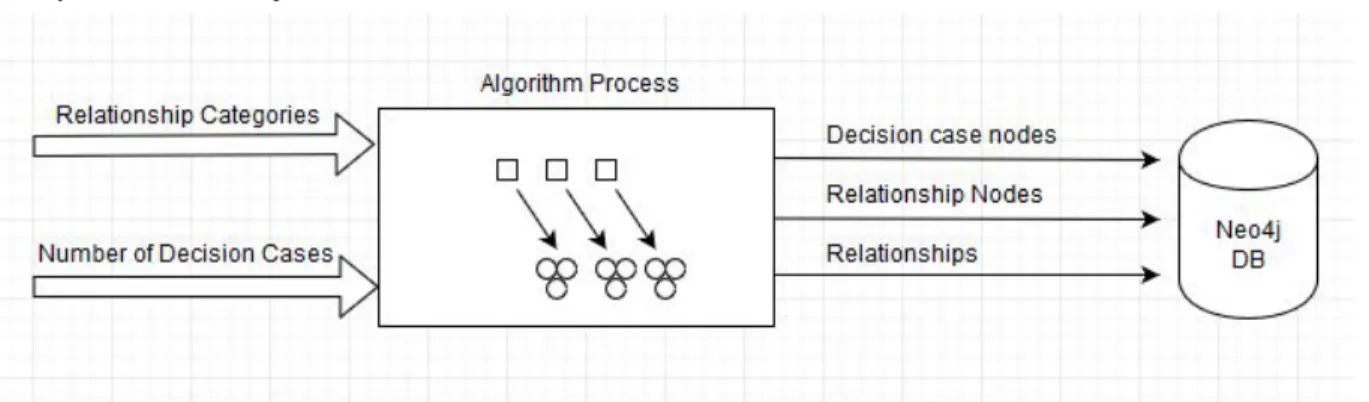
Below in Figure 6 we provide a diagram that displays the input and output from the algorithm and how it is finally sent to the Neo4j database.
Figure 2: Input and Output visualisation of the decision case creation process.
The first input is the relationship categories that are contained in our Excel file. The second input is the input argument for the algorithm which determines how many decision cases are generated. The algorithm then proceeds with the randomisation, and generation, of nodes and relationships for each decision case. The result is three datasets, which consists of the decision case nodes, the relationship nodes and the relationships. This was a brief overview of the algorithms input and output; all parts will now be explained in greater detail.
7.2 Using Excel Files to Store the Primitive Data
The algorithms needed a knowledge base that they could use to generate decision cases from. We decided to put the analysed information into excel files. The test data provided in appendix A represent the category primitives in the excel table structure.
The excel files are used as the base data template that the algorithms use for the generation. The rows and columns of these files are interpreted by the algorithms where each row represents a possible node, e.g. a primitive, that is a member of one of the five categories. These nodes describe the attributes of decision cases. For example, the Role category classifies entities that are involved in the activity that the decision case node is describing. Let us say that this case is to develop some software, then a Role node could be the initiator of that development project, e.g. CEO, specifically the decision case node would have a relationship to the Role node that has the name: Initiator. And the Role node itself would be named: CEO. All the categories work together to provide an overview of everything that has affected a certain activity, e.g. if a project has outsourced elements or if it is created completely in-house, how the product is supposed to be used and so on.
William Achrenius Graph Generation Algorithms Martin Bergman Törnkvist for the Grade Decision Canvas
7.3 Random Generation
Using excel files we created a method of reading nodes and relationships from a file. This made it possible to generate documented decision cases directly from file without using neo4js cypher language. Instead all generation is made through our modified version of the GraphAware library [22].
The excel files provided a convenient way of structuring input, although using it for generating many different decision case variants would mean that one file for each variant must be created. We concluded that generating multiple different decision cases without predetermining all the elements would need automated randomisation. The files did not only aid in structuring the input, but also in structuring the decision case metadata. Using what we had analysed from the decision canvas we created one file that would contain all the metadata for all possible nodes that a decision case could have a relationship to. We constructed the file in this way because in GRADE the decision case node is always the centre point and does not have any relationships directed towards it. This is the file that is presented in appendix A and serves as the primary metadata file for our random generation algorithm. Note that the file does not contain any metadata information on the decision cases. The reason for this is that the properties of the decision cases themselves are not as important. This will become clearer when the process of the algorithm is explained. The file contains the information needed to create a relationship and has room for additional properties, if required. The essential information is a node label, a node name and the name of the relationship itself. Other additional properties are optional. Both nodes and relationships can have several properties.
The properties such as the name of the node is interpreted by our algorithm using certain tools of randomisation. The name property of the relationship nodes, which is displayed within the node in Neo4j’s graphical view, is sent to a randomiser, which is called a faker, that determines what type of random value is appropriate for that name. Our faker works with seeds based on third party libraries. For example, if the name is “Decision stakeholder” the faker could replace it with the name “CEO”. This faker service already existed in the GraphAware algorithms. The faker has been edited to fit the GRADE metadata.
7.4 Algorithm Process Overview
We created several algorithms for generating decision cases, we will describe the one that we used for our comparison, which is a random generation algorithm that is based on the previously mentioned metadata file. This algorithm accepts one argument, an integer. The integer indicates how many decision cases that will be created by the algorithm. The algorithm operates in three stages. Firstly, we create several decision cases based on the argument given. Secondly, we read the metadata file and create relationship nodes, randomising the properties of the nodes using our faker service. Lastly, we start generating the relationships between the decision case nodes and the relationship nodes.
The generating of the relationships is where we have experimented with different values because it contains several random elements. For each of the decision case files we want to go through all the possible relationship nodes and create some number of relationships. Our initial premise is that for each of the relationship node there is a 50% chance that it creates the relationship the current decision case and that node. If a relationship succeeds in being created it has a chance of creating either zero, one, two or three additional nodes of the same kind as the current relationship being created. The additional nodes created get a relationship created from the current decision case node and one other additional relationship, of the same kind, from another randomly selected decision case.
The name values of these additional nodes are randomised to make them be different in name but equal in category. There are exceptions to the creation of the additional nodes. Because of logical reasons some node
William Achrenius Graph Generation Algorithms Martin Bergman Törnkvist for the Grade Decision Canvas
categories are prohibited from being duplicated. An example of this would be if a project has expert-based input. Expert based is a statement and not an entity with a name that can be randomised, therefore it is not necessary for the case decision to have two or more of them.
To control the relationship creation, so that it is not possible to get zero relationships, there is a failsafe in place that ensures that there is always one relationship node of each category. This functionality is independent of the additional relationship node generation and creates only one relationship from the current decision case node to the category that did not receive a relationship through the 50% chance.
7.5 Pseudocode
Details of the process will now be explained for each part of the pseudocode, the complete pseudocode can be found in appendix B.
Figure 3: Row 1 to 6, pseudocode of the algorithm.
The algorithm starts by initialising several decision case nodes. The decision case nodes are named by using “Case” plus a random number added to it. On row six a function is called that handles the reading of our Excel file, found in appendix A. The result of this is an array of possible relationships.
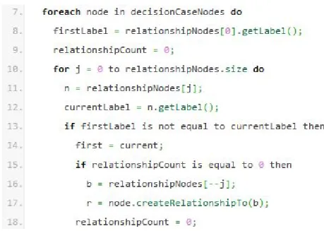
Figure 4: Row 7 to 18, pseudocode of the algorithm.
The primary loop of the algorithm iterates once for each of the decision cases. Row eight through row 18 constitutes the failsafe that makes sure there is at least one relationship of each label category. The label category is given by the first column of our Excel file. If the name in this column remains the same, for any number of rows, it is counted as one category. For example, the first five rows of the excel file has the name
William Achrenius Graph Generation Algorithms Martin Bergman Törnkvist for the Grade Decision Canvas
DECISION_GOAL, the 6th row will trigger the relationships check. When the category changes, if no
relationships were selected, the if clause on row 15 will guarantee that a relationship is created of the previous category. The last row of the previous category will be selected.
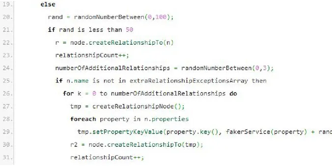
Figure 5: Row 19 to 31, pseudocode of the algorithm.
From row 19 and onwards contains the main part of the generation. Using the array of possible relationship nodes, there is a 50% chance a relationship is created between the decision case node and each relationship node. If the randomisation is successful it continues with additional relationship generation on row 24. The number of additional relationships is random and limited to three, based on our experimentation. Row 25 checks for exceptions to making additional relationships of a node category.
Figure 6: Row 32 to 38, pseudocode of the algorithm.
Row 33 through 37 creates the extra connection between a randomly selected decision case and the additional relationship. This part of the generation process is important and causes several decision cases to be able to share multiple properties. Lastly, the r, r2 and r3 variables serve to describe the relationships as data entities and are part of the relationships array. When the algorithm completes it returns the decision case nodes, relationship nodes and relationships.
William Achrenius Graph Generation Algorithms Martin Bergman Törnkvist for the Grade Decision Canvas
8.
Results
To compare the graphs created by the algorithm and the graphs existing in the example database we have analysed the decision cases in two ways. The first method is comparing the number of nodes and relationships between the algorithm created decision case and a typical decision case from the pre-existing, manually created, data repository. The second method is by an empirical comparison between the properties and relationships in a decision case that has been created by the algorithm and a decision case that exist in the example database.
8.1 Number of Nodes and Relationships
Since the number of nodes and relationships created by the database is randomised the generation has been done three times respectively for one, five and ten decision cases. As can be seen in appendix A our algorithm uses 10 different node label names and 14 different relationship types. The chance to create a second node is the
previously mentioned 50% chance for each node with a maximum of three nodes generated for each node label. The exceptions are the node labels that are locked to one creation. With these values the measured number of nodes and relationships are displayed below.
Decision
Cases Node Labels Relationship Types Nodes Relationships Time (ms)
1 10 14 33 32 73 1 10 14 30 29 61 1 10 14 26 25 52 5 10 14 103 210 85 5 10 14 114 224 79 5 10 14 102 198 70 10 10 14 149 368 66 10 10 14 185 448 59 10 10 14 180 420 64
Table 1: Results from counting the number of nodes and relationships from artificial decision cases created by our algorithm.
One of the first things that can be noted is the fact that the amount of relationships created for the single decision cases is always the number of nodes minus one. This is logical because the algorithm does not create multiple relationships to the same node, and at the same time it will never create a relationship to the decision case node itself, later in the paper we will talk more about why it is that no more than one relationship is created for each node. Taking these things into account means that the extra node counted among the nodes is the decision case node.
The generation of five and ten decision cases did see a substantial increase in relationships generated. This is to be expected because of the relationships going between the decision cases and the nodes that they share. A greater number of generated decision cases will result in more shared nodes which means that the difference between the number of nodes and relationships will increase.
The measured execution time was varying and did not seem to be affected by the number of nodes generated. While looking at the measured values it is not apparent why this is the case, a logical conclusion would be that more nodes generated would result in an increased generation time.
William Achrenius Graph Generation Algorithms Martin Bergman Törnkvist for the Grade Decision Canvas
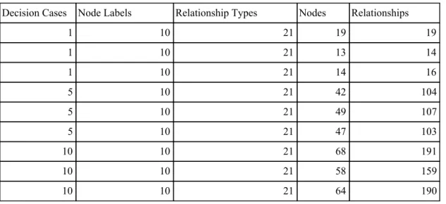
Decision Cases Node Labels Relationship Types Nodes Relationships
1 10 21 19 19 1 10 21 13 14 1 10 21 14 16 5 10 21 42 104 5 10 21 49 107 5 10 21 47 103 10 10 21 68 191 10 10 21 58 159 10 10 21 64 190
Table 2: Results from counting the number of nodes and relationships from decision cases taken from the manual data repository.
Here we can see that the number of relationships is equal or more than the number of nodes. One might think this is because the example database is using 21 different relationship types instead of our algorithm that is using 14, but this would be a false assumption. The reason for the difference between the number of relationships between the decision cases is because the example database has instances of multiple relationships from the decision case to a single property. Something that our algorithm does not create, our algorithm solves this by a different method that will be explained later.
8.1.1 Minimum and Maximum Number of Nodes and Relationships
Because of the nature of the algorithm, and the restrictions that have been put on it, there exists a minimum and maximum number of nodes and relationships that can be generated depending on the number of decision cases generated. The minimum number is only affected by the number of unique labels that we have under Label
Name, displayed in appendix A, we currently have 10 unique label names.
The maximum number of nodes is however affected by three things. The first is the total amount of labels that we have under Label Name in appendix A, this is currently 42. The second is the maximum number of nodes that can be created for each label name, this is currently set to three. The second additional is the number of restrictions that has been put on the node categories. We previously mentioned the restrictions and how it is a necessary addition to create logical decision cases. The current categories that we have restricted from being multiplied are the following:
{Innovation and Learning, Strategic, Tactical, Operational, Reuse, Adapt, Buy, Develop, In-house, Outsource,
Open Source, COTS, Project-based, Inner Source, Subcontracting, Crowd-source, Expert-based, Memory-based, Parametric, Non-parametric}
For the sake of calculating the maximum number of nodes and relationships that can be created it is required to take these 20 categories into account since they are only able to be created once, instead of three times, for each decision case.
From these observations it is now possible to calculate the minimum and maximum number of nodes and relationships for any amount of decision cases generated. The minimum could be mathematically displayed as following:
inimumNodes umberOfUniqueLabels NumberOfDecisionCases NumberOfDecisionCases
William Achrenius Graph Generation Algorithms Martin Bergman Törnkvist for the Grade Decision Canvas
inimumRelationships umberOfUniqueLabels NumberOfDecisionCases
m = N *
The maximum could be mathematically displayed as following:
maximumNodes = ((NumberOfDecisionCases NumberOfLabels) + ((NumberOfLabels -*
NumberOfRestrictions) 3) NumberOfDecisionCases* +
maximumRelationships = ((NumberOfDecisionCases * NumberOfLabels) + ((NumberOfLabels - NumberOfRestrictions) 3)*
Using this we can calculate the minimum and maximum number of nodes and relationships possible for the displayed decision cases in Table 1.
Decision Cases Minimum Number of Nodes Minimum Number of Relationships Maximum Number of Nodes Maximum Number of Relationships 1 11 10 87 86 5 55 54 281 276 10 110 109 496 486
Table 3: The minimum and maximum number of nodes and relationships for one, five and ten artificially generated decision cases.
8.2 Properties and Relationships
In this section we do a comparison between the different kind of nodes and relationships that are used by our artificial decision cases and the decision cases from the example database. We will break down a single decision case from each and compare them. Starting with a decision case that has been artificially generated.
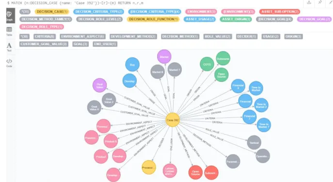
Figure 7: Case 392 that has been artificially created by our algorithm. The middle node is the decision case node and surrounding it is its properties. The decision case is connected to its properties using vectors that represent their relationships.
William Achrenius Graph Generation Algorithms Martin Bergman Törnkvist for the Grade Decision Canvas
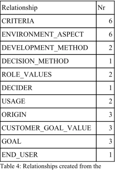
Now to break down this decision case. Looking at it we can see that it is using 11 out of the 14 possible relationship types and it has created 30 relationships to 30 different nodes. The relationships created are displayed in table 4. Relationship Nr CRITERIA 6 ENVIRONMENT_ASPECT 6 DEVELOPMENT_METHOD 2 DECISION_METHOD 1 ROLE_VALUES 2 DECIDER 1 USAGE 2 ORIGIN 3 CUSTOMER_GOAL_VALUE 3 GOAL 3 END_USER 1
Table 4: Relationships created from the artificial decision case displayed in figure 7.
CRITERIA. The algorithm has created 6 CRITERIA relationships, three of which are connected to Financial,
Financial 3 and Financial 7. Since the algorithm’s faker service is currently not equipped with examples for all different properties the algorithm will differentiate between different kinds of similar properties by adding a random number after the property. The same can be seen for the three other criteria nodes which are Time to Market, Time to Market 2 and Time to Market 7. Each of these simulates different kind of Time to Market properties that are connected to the decision case by the criteria relationship.
ENVIRONMENT_ASPECT. There are 6 different environment aspects that has been generated by the
algorithm. The first two are related to the product by the nodes Product and Product 5. The second two are Process/Business Analyst and Process/Business Analyst 2. The last two are Development Technology and Development Technology 0. All of these are environment properties, meant to describe the context of the decision case. The Process/Business Analysts described in the context are therefore non-decision properties. They are not related to the decision-making itself, they are only there to clarify the context of the decision case.
DEVELOPMENT_METHOD. The algorithm has generated two development methods for the decision case.
One is Open Source and the other is Subcontracting. Worth noting is that both properties are included in the list of prohibited properties which means that they can only occur once, just like they have done here.
DECISION_METHOD. The algorithm has only generated one decision method which is the Parametric
property, this is also one of the prohibited properties.
ROLE_VALUES. Two role values have been generated, Tactical and Operational, both of which are prohibited
properties.
DECIDER. One decider has been generated which is a Process/Business Analyst. It is important to understand the difference between the previous Analysts generated with the environment aspect relationship and the analyst generated with the decider relationship. The relationship helps to clarify what the relationship is between the
William Achrenius Graph Generation Algorithms Martin Bergman Törnkvist for the Grade Decision Canvas
decision case and the properties. In this case the Analyst has a key role in the decision-making, instead of the previous non-decision Process/Business Analysts, generated with the environment aspect relationship, that does not have an active role in the decision-making process.
USAGE. Two usage properties have been generated, Buy and Develop. The usage relationship is describing the
asset usage, as in how the asset will be used. Both are prohibited properties.
ORIGIN. The decision case has three origin properties, Open Source, COTS (Commercial-off-the-shelf) and
Outsource. All three of which are prohibited properties.
CUSTOMER_GOAL_VALUE. Three customer goal values have been created, Goal Value, Goal Value 0,
Goal Value 2.
GOAL. The decision case has three goal properties, Market, Market 7 and Market 9. Representing three different market goals.
END_USER. The algorithm has generated one end user. This is one of the properties that can use the original faker service from the library. The node name is Lehner, Lehner and Lehner which is a randomly generated company name that represents the end user.
8.3 Decision Case from the Manually Created Data Repository
There are 77 decision cases to pick from in the example database, for this comparison we have tried to pick a case that is as general as possible and gives a fair representation for the kind of decision cases that can be found in the database.
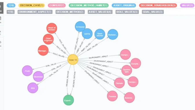
Figure 8: A decision case picked from one of the 77 cases in the example database.
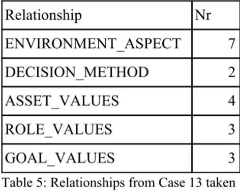
This is Case 13 from the manually created data repository. We can see that this decision case is using 5 different relationships out of the total 21 relationships that can be found in the data repository. The decision case has a total of 19 nodes and 19 relationships.
William Achrenius Graph Generation Algorithms Martin Bergman Törnkvist for the Grade Decision Canvas
Relationship Nr ENVIRONMENT_ASPECT 7 DECISION_METHOD 2 ASSET_VALUES 4 ROLE_VALUES 3 GOAL_VALUES 3
Table 5: Relationships from Case 13 taken from the manually created data repository.
ENVIRONMENT_ASPECT. This decision case has 7 different environment aspects, Domain, Complexity,
System type, Component usage, Component history, Accessibility and Process.
DECISION_METHOD. The decision case has two decision method relationships but as we can see they are
pointing to the same node with the name Expert-based. The relationships created have different decision types, Quality and Financial. Both Financial and Quality are properties that are used in the artificial decision case but displayed in a different manner. The algorithm will instead of generating extra relationships to the same node generate a new node with the same relationship. The artificial decision case would instead create one
relationship named DECISION_METHOD that is relating to a node called Expert-based, this is similar so far. But instead of generating two relationships to this Expert-based node, with different decision types as properties, it would create two additional relationships with the name CRITERIA, relating to nodes with the labels Quality and Financial, to explain the same thing. The visual aspect is different, but the meaning is the same.
ASSET_VALUES. There are four different asset values, Open source, COTS, In-house and Outsource. These
properties are like the ones used with the ORIGIN relationship in the artificial decision case.
ROLE_VALUES. The decision case has three role values, Head of division, Chief engineer and Management.
These are some of the values that our algorithm is currently missing, because of the lack of an extended faker service. The artificial decision case would simply create nodes named either Strategic, Tactical or Operational to explain this node.
GOAL_VALUES. The final relationship is pointing towards the last three nodes. These are Decrease Cost,
Profit and ROI. The same case stands for these nodes as the one with the role value relationship. An extended faker service would be able to generate examples of different role values for the artificial decision case. Right now, it would simply generate nodes that we have seen above, Financial with a random number to indicate if there are multiple financial goals. Another possibility is that it creates a node with the name Innovation and Learning since that is also one of the possible goal values in our data file, see appendix A.
William Achrenius Graph Generation Algorithms Martin Bergman Törnkvist for the Grade Decision Canvas
9.
Discussion
The values that the algorithm uses for the randomisation, e.g. 50% relationship chance and the chance to create additional relationships, provide the similarities that we were looking for, regarding the comparison and the resulting behaviour. The purpose of the work and the algorithm was to be as similar as possible to the
pre-existing, manually created, data repository. The values can, in their worst case, generate decision cases that can be extreme in the average case, however, we do not deem this to be disruptive to the overall usage of the algorithm. It provides a fast generation, less than 100 milliseconds on average, of decision cases and relationships that can be used for analytic work. It is also able to provide acceptable amounts of data that are required for the artificial data analysis.
It is important to note that if any of these randomisation values should be changed all, the metrics and results of this work would not correspond correctly to the result of the changed version. We do not discourage this, it is possible to change and adapt the generation algorithm to fit other scientific models that can use graphs as representation. This inherently demands some sort of alteration. Further recommendations on how and what to change in the algorithm, and how they affect each other, is provided under future work.
Another component to the algorithm, that is one of the shortcomings of this work, is the use of the faker service. It was provided by GraphAware [22]. It ended up being altered many times during the work. Regarding the GRADE decision case model, it did not provide many fitting random values that could be used. The result included using the original faker behaviour for a few of the metadata categories. We extended the behaviour with an additional small list of values that could be used for one of the categories, namely the Role category. This category is one of those not included in the list of relationship exceptions, which means that it can be duplicated during generation. It makes up half of the sub-categories that can be duplicated. We decided to create a small list of names that could be used for generating Roles, although this list makes the result look better, it can be extended. Each of the categories that can be duplicated would benefit from having their own library of randomisation. It would be advantageous if a faker service was made specifically for the GRADE decision case model or any other scientific model that the generation is adjusted for.
William Achrenius Graph Generation Algorithms Martin Bergman Törnkvist for the Grade Decision Canvas
10. Conclusions
The development of computer architecture as a field has led to the involvement of several entities in the decision-making progress. To adapt to the new requirements of architectural decision, models have been developed. These models provide categorization and classifications of different elements and aspects that affect a decision case. One such model is the GRADE decision canvas. Using this model represented through graphs, with nodes and relationships, the essential elements of a complex case can be structured be analysed.
Using a graph system called Neo4j in combination with the GRADE decision canvas, we have created a plugin that uses algorithms to generate randomised decision cases and relationships. The decision cases generated can then later be used to analyse typical decision cases.
To make our algorithm as realistic as possible we compared it to a pre-existing data repository containing decision cases that was manually created by one of the researchers behind GRADE. Firstly, the weight between the number of nodes and relationships were compared. Secondly the decision cases were compared by looking at what kind of nodes and relationships exist. The result shows that our algorithm generates, on average, more relationship nodes, instead of generating multiple relationships to the same relationship node. An example of this is the dual decision method relationships that exist in Case 13 in the manual data repository. The dual relationships are used to explain that both a Quality and Financial decision method is expert based. The artificial algorithm would explain this occurrence in another way by generating three nodes, two of which are named Quality and Financial and one of which are named Expert-based. The Quality and Financial nodes would be connected to the decision case by the relationship called CRITERIA and the Expert-based node would relate to the decision case with the relationship called DECISION_METHOD, the same relationship as in the manual decision case. Together these nodes and relationships would explain the same thing, that the criteria for the decision method are Quality and Financial. Our algorithm creates on average more nodes, around 15 to 20 relationships per case, than that of the cases in the manual database have. One of the reasons for this is that we do not create dual or triple relationships, which exist in the manual database.
The randomisation values used within our algorithm are directly related to the result. The algorithm is also open for modification if anyone should want to change these values. It can also be adapted for any other scientific architectural model. There is no limit to how many nodes that can be generated in this way. This can put a strain on the graphical viewer of Neo4j. Since great amounts of data are needed for artificial data analysis there was no incentive to throttle the generation.
The current faker service does not provide randomisation of values for all categories since many require highly complex randomisation.
William Achrenius Graph Generation Algorithms Martin Bergman Törnkvist for the Grade Decision Canvas
11. Future Work
There are several things that can be developed further. The randomisation algorithm has three components that affect the behaviour of the generation the most. The first is the chance that a relationship is created, the second is the amount of additional relationship nodes that can be created and lastly the types of relationships that are excluded from being duplicated. As of now these values are hardcoded into the algorithm. The values that we used for these aspects are what we concluded to be the most balanced, for generating a similar data repository, as to the repository that we used for our comparison. This was the intended goal of our work; however, these values can be set up to be whatever the user wants. We do not recommend values that are several times larger than ours. The reason for this is that the values are multiplicative in relation to the execution time of the algorithm.
The first component, e.g. the 50% chance value, can be more freely changed. Mostly because of the failsafe that at least one relationship of every category is created. The second component affects the number of times a relationship is duplicated, dependent on the chosen value, which can dramatically increase the maximum number of nodes that can be created. Be careful with this since, if this number is increased, the number of nodes that can be created is increased relative to the amount of node categories that are defined in the metadata file. If there are 40 categories and the duplication amount is increased by 2 the number of nodes that can be created will be: 2 x 40. The last component, which is the list of nodes that can be duplicated, is the most customizable one. If the metadata file is extended, new relationships might only be required once per decision case and can be added to the list. This is entirely up to the user, in what they see appropriate to be duplicated or not.
If changes are made to the algorithm or the metadata file, the faker service used would possibly need to be changed as well. We did not use randomisation for all values since are require complex randomisation. Instead we complemented the faker by adding values in the form of small tables that can be selected at random for some of the nodes’ names. Any future work could include extending the available randomisation with their own values and identifiers.
William Achrenius Graph Generation Algorithms Martin Bergman Törnkvist for the Grade Decision Canvas
12. References
[1] R. Capilla, A. Jansen, A. Tang, P. Avgeriou, M. A. Babar. “10 years of software architecture knowledge management: Practice and future,” Journal of Systems and Software, vol. 116, June 2016, pp. 191–205. [2] D. Tofan, M. Galster, I. Lytra, P. Avgeriou, U. Zdun, M.-A. Fouche, R. de Boer, F. Solms. “Empirical Evaluation of a Process to Increase Consensus in Group Architectural Decision Making,” Information and
Software Technology. vol. 72, April 2016, pp. 31–47.
[3] M. Nowak, C. Pautasso. “Team Situational Awareness and Architectural Decision Making with the Software Architecture Warehouse,” in Proceedings of the 7th European Conference on Software Architecture, ECSA’13, Montpellier, France, July 1-5, 2013, pp 146-161.
[4] P. Krutchen. “An Ontology of Architectural Design Decisions in Software Intensive Systems,” Proceedings
of the 2nd Groningen Workshop on Software Variability Management, Groningen, Netherlands, December 3-4, 2004, pp. 54–61.
[5] R. C. De Boer, R. Farenhorst, P. Lago, H. Van Vliet, V. Clerc, A. Jansen. “Architectural knowledge: Getting to the core,” in Third International Conference on Quality of Software Architectures, QoSA 2007, Medford, MA, USA, July 11-23, 2007, pp 197–214.
[6] E. Papatheocharous, K. Petersen, J. Axelsson, C. Wohlin, J. Carlson, F. Ciccozzi, S. Sentilles, A. Cicchetti. “The GRADE Decision Canvas for Classification and Reflection on Architecture Decisions,” in Proceedings of
the 12th International Conference on Evaluation of Novel Approaches to Software Engineering, ENASE 2017, Porto, Portugal, April 28-29, 2017, pp. 187-194.
[7] E. Papatheocharous, K. Petersen, A. Cicchetti, S. Sentilles, S. M. A. Shah, and T. Gorschek. “Decision support for choosing architectural assets in the development of software-intensive systems: The GRADE taxonomy,” in Proceedings of the 2015 European Conference on Software Architecture Workshops, ECSAW 2015, New York, NY, USA, 2015. Available: https://dl.acm.org/citation.cfm?id=2797483
[8] E. Papatheocharous, K. Wnuk, K. Petersen, S. Sentilles, A. Cicchetti, T. Gorschek, S. M. A. Shah. “The GRADE taxonomy for supporting decision-making of asset selection in software-intensive system
development,” Information and Software Technology, Volume 100, August 2018, pp. 1-17.
[9] R. Angles and C. Gutierrez. “Survey of graph database models,” ACM Computing Surveys (CSUR). vol. 40, February 2008, pp. 1-39.
[10] Db-engines.com, DB-Engines Ranking - popularity ranking of database management systems, 2018, [Online] Available at: https://db-engines.com/en/ranking, [Accessed Apr 06, 2018].
[11] C. Mayr, U. Zdun, S. Dustdar. “Reusable architectural decision model for model and metadata
repositories,” in 7th International Symposium on Formal Methods for Components and Objects, FMCO 2008, Sophia Antipolis, France, October 21-23, 2008, pp. 1–20.
[12] O. Zimmermann, T. Gschwind, J. Kuester, F. Leymann, N. Schuster, “Reusable architectural decision models for enterprise application development,” in Third International Conference on Quality of Software
Architecture, QoSA 2007, Medford, MA, USA, July 11-23, 2008, pp. 15–32.
[13] N. Mansour and M. Salame, “Data Generation for Path Testing,” Software Quality Journal, vol. 12, pp 121-136. June 2004.
[14] R. Zhao and Q. Li, "Automatic Test Generation for Dynamic Data Structures," in 5th ACIS International
Conference on Software Engineering Research, Management & Applications (SERA 2007), Busan, August 20-22, 2007, pp. 545-549.
[15] S. Sai-ngern, C. Lursinsap and P. Sophatsathit, “An address mapping approach for test data generation of dynamic linked structures,” Information and Software Technology, vol. 47, pp 199-214. March 2005.
[16] S. Marzukhi, R. A. Hazwani, N. Wahida, S. I. Shafikah, Z. Zainol and P. N. Ellyza. "Automatic Artificial Data Generator: Framework and implementation," 2016 International Conference on Information and
Communication Technology (ICICTM), Kuala Lumpur, May 16-17, 2016, pp. 56-60.
[17] D. R. Jeske, B. Samadi, P. J. Lin, L. Ye, S. Cox, R. Xiao, T. Younglove, M. Ly, D. Holt, and R. Rich. “Generation of synthetic data sets for evaluating the accuracy of knowledge discovery systems,” in Proceedings
of the eleventh ACM SIGKDD international conference on Knowledge discovery in data mining (KDD '05), ACM, New York, NY, USA, August 21-24, 2005, pp. 756-762.
William Achrenius Graph Generation Algorithms Martin Bergman Törnkvist for the Grade Decision Canvas
[18] M. Verstraaten, A. L. Varbanescu and C. de Laat, “Synthetic Graph Generation for Systematic Exploration of Graph Structural Properties,” in Euro-Par 2016 International Workshops, Grenoble, France, August 24-26, 2016, pp. 557-570.
[19] K. O. Stanley and R. Miikkulainen, “Evolving neural networks through augmenting topologies,”
Evolutionary Computation, vol. 10, pp. 99-127, June 2002.
[20] D. A. Bader and K. Madduri, “Design and Implementation of the HPCS Graph Analysis Benchmark on Symmetric Multiprocessors,” in 12th International Conference, Goa, India, December 18-21, 2005, pp. 465-476.
[21] D. I. K. Sjoberg, T. Dyba, M. Jorgensen, “The future of Empirical Methods in Software Engineering Research,” in Future of Software Engineering, Minneapolis, MN, USA, May 23-25, 2007, pp 358-378. [22] Neo4j Graphgen Procedure. Internet: https://github.com/graphaware/neo4j-graphgen-procedure, Jun. 29, 2016 [Accessed Apr 06, 2018]
[23] GRADE Neo4j Graphgen Procedure. [Online] Available:
https://github.com/Wilach/GRADE-neo4j-graphgen-procedure, May 23, 2018 [Accessed May 23, 2018].
William Achrenius Graph Generation Algorithms Martin Bergman Törnkvist for the Grade Decision Canvas
Appendices
Appendix A
Figure 9: Excel file containing metadata of node categories.
The above picture is our test data Excel file. This file contains the metadata that is required to create our relationship nodes and generate decision cases. Each row describes an identified primitive within the five classifications. How they are related can be derived from the Label Name column. The first five rows have the label name DECISION_GOAL and refer to the Goal classification that describes important goals to consider when making an architectural decision. The next 10 rows describe Roles, then Assets, Decision method and
criteria and lastly Environment. The other parts of the labels can be called subcategories, this is just to give additional detail to the categories. The rest of the columns are properties that are formatted as key: value pairs. The Node name column gives us the name value that is displayed on the node when in the graphical view. It is the value that is given to the faker service so that an appropriate random name can be generate for the node. The
relationship property is used as the name of the relationship, the value that is displayed on the relationship vector. The rest of the columns are optional properties, although it is recommended to have the symbol property
William Achrenius Graph Generation Algorithms Martin Bergman Törnkvist for the Grade Decision Canvas
since it provides additional categorization. More properties can be added by extending the document with extra columns. More categories can also be added by extending the document with additional rows.
William Achrenius Graph Generation Algorithms Martin Bergman Törnkvist for the Grade Decision Canvas