ARTIFICIAL INTELLIGENCE FOR VERTICAL FARMING – CONTROLLING THE FOOD PRODUCTION

S

CHOOL OF

I

NNOVATION

,

D

ESIGN AND

E

NGINEERING

V

ÄSTERÅS

,

S

WEDEN

Thesis for the Degree of Master of Science (60 credits) in Computer Science |

DVA429

ARTIFICIAL

INTELLIGENCE

FOR

VERTICAL

FARMING

–

CONTROLLING

THE

FOOD

PRODUCTION

Rami Abukhader; Samer Kakoore

Rar19002@student.mdh.se

;

Ske19003@student.mdh.se

Examiner:

Mikael Ekström

Mälardalen University, Västerås, Sweden

Supervisor: Baran Cürüklü

Mälardalen University, Västerås, Sweden

Company Supervisor: Sepher Mousavi

Swegreen, Stockholm, Sweden

Abstract

The Covid-19 crisis has highlighted the vulnerability of access to food and the need for local and circular food supply chains in urban environments. Nowadays, Indoor Vertical Farming has been increased in large cities and started deploying Artificial Intelligence to control vegetations remotely. This thesis aims to monitor and control the vertical farm by scheduling the farming activities by solving a newly proposed Job-shop scheduling problem to enhance food productivity. The Job-shop scheduling problem is one of the best-known optimization problems as the execution of an operation may depend on the completion of another operation running at the same time. This paper presents an efficient method based on genetic algorithms developed to solve the proposed scheduling problem. To efficiently solve the problem, a determination of the assignment of operations to the processors and the order of each operation so that the execution time is minimized. An adaptive penalty function is designed so that the algorithm can search in both feasible and infeasible regions of the solution space. The results show the effectiveness of the proposed algorithm and how it can be applied for monitoring the farm remotely.

Table of Contents

1.

Introduction ... 5

1.1.

Problem Formulation ... 5

1.1.1.

Research Questions ... 5

2.

Background ... 7

2.1.

Indoor vertical farming ... 7

2.2.

Unsupervised learning ... 7

2.3.

Evolutionary algorithms ... 7

2.4.

Genetic algorithms ... 8

3.

Related Work ... 9

4.

Method ... 10

4.1.

Proposed scheduling genetic algorithm ...10

4.1.1.

Chromosome representation ... 11

4.1.2.

Creation of the population ... 11

4.1.3.

Parents selection... 11

4.1.4.

Off-spring generation ... 12

4.1.5.

Mutation ... 12

4.1.6.

Fitness function ... 13

4.1.7.

Constraint satisfaction ... 13

4.1.8.

Termination criteria ... 13

4.2.

Applying the algorithm on vertical farming...14

5.

Results and Evaluation ... 15

5.1.

Scheduling 12 operations ...15

5.2.

Scheduling 24 operations ...16

6.

Discussion ... 18

7.

Conclusions ... 19

References ... 20

List of Figures

Figure 1. Structure of the new IVF systems [6]. ... 7

Figure 2. A general schematic for an evolutionary algorithm [10]. ... 8

Figure 3. The process of Swegreen’s vertical farm ... 14

Figure 4. The evolution process after 27 epochs ... 15

Figure 5. Gantt chart of the optimal solution for scheduling 12 operations ... 15

Figure 6. Gantt chart of the optimal solution for scheduling 24 operations ... 17

Figure 7. The evolution process of idle time and the penalty function of running 24 operations ... 17

Figure 8. Air cycling job example on the farm ... 18

List of Tables

Table 2. Processors properties structure ... 11

Table 3. Task properties structure ... 11

Table 4. The process of Swegreen’s vertical farm ... 11

Table 5. The operations used in the research ... 14

Table 6. Output solution of 12 operations from the program ... 15

1. Introduction

The world population is rapidly increasing and predicted to be 9 billion by 2050, of which 70% will live in urban areas, this change alongside climate change will affect the earth resources, especially the food supply chain [1]. Food security for countries that depend on food import, such as Sweden, is subject under high risks when the global supply chains are affected by a crisis like COVID-19, climate change and population increase. These crises require new methods to solve the food supply chain shortage in urban areas. Agriculture is being carried out in indoor vertical farming systems that produce faster, cheaper, and healthier plants than in normal conditions, the importance of these crops demand fresh and healthy vegetables and herbs at the local level [2]. Vertical farming is a new promising solution for countries with food security problems [1].

NeighbourFood (NF) project is an Indoor Vertical Farm (IVF) that produces vegetables and herbs based in Stockholm and aims for food production. Also, it has an ambition of interacting with its customers, i.e., food retails, restaurants, and ordinary citizens. The proposal assumes the concept of Farming as a Service (FaaS), which means that farming becomes a service and by that (1) generates new services, (2) contributes to the creation of a sharing economy platform including neighbours for neighbours (the producers and consumers). The IVF in this project controls all growth factors such as water, light, temperature, humidity, and CO2. A sensor is attached to the plants for gathering data. Later the data is visually inspected by the operator. The challenge in the assumed IVF is that it is labor-intensive, thus automation is highly desired. Thus, there are a need for Artificial Intelligence (AI) solutions to control and predict food production.

The Job-shop scheduling problem (JSP) is one of the best-known combinatorial problems and it is considered a strongly NP-hard problem [3]. The JSP was introduced by Graham in 1966 [4]. It can be represented as a set of jobs j are processed on a set of processors p and each job is composed of a set of operations 𝑂 = 𝑜1, 𝑜2, 𝑜3, . . . , 𝑜𝑛. Each processor can process only one operation at a time, while the operations have a certain order (dependency) that cannot be processed until the previous operation order is completed. There are a variety of real-world applications that lead to extended job-shop scheduling models, such as Flexible manufacturing, Multiprocessor task scheduling, Railway scheduling, and Air traffic control that can be described in [5].

This thesis will focus on generally solving the scheduling problem by implementing an algorithm that could solve complex problems or scenarios. The solution to the problem will enhance the indoor vertical farm by scheduling the farming process and farm activities by deploying the implemented algorithm. The proposed solutions can also help to control food production during crises such as COVID-19 since access to labor is, as we have seen, a challenge. The thesis will be done in collaboration with Swegreen Company.

1.1. Problem Formulation

The objective of the thesis is to investigate and apply a population-based search algorithm, Evolutionary Algorithm (EA), to plan the farm’s activities in order to schedule the harvests, i.e., the food production with high accuracy and precise results.

The scope of this study has several objectives. On the first hand, it is important to investigate a model that can solve the scheduling problem that finds the best order of operation and assign the processor to compute each operation. On the second hand, apply the algorithm to schedule the farm activities so we can measure the required number of resources used in the farming process and how it depends on each other to produce fresher and healthier vegetables and herbs, which will show how the vegetation is doing during the farming process. Finally, we want to evaluate the results and write a conclusion.

1.1.1. Research Questions

To address the described problems, some initial research questions have been defined which are listed below: • RQ1: What is the suitable implementation of the EA technique to control food production until the next

harvest?

• RQ2: How can we predict the time to next harvest?

• RQ3: How could this EA technique enhance food productivity?

The paper is organized as follows. Section 2, a brief background of the necessary knowledge to place in thesis paper within the proper context. Not all the mentioned sectors may be used in the implementation process. The purpose of this knowledge is to establish a foundation of concepts and terminology to facilitate the comprehension of the actual work. Section 3, a review on the subject and comparison of this paper with other previous researches. Section 3, a presentation of the algorithm, by detailing the strategies of the genetic algorithm to generate the initial population and represent the problem, the fitness function, selection criteria, and linking the problem to vertical farming. Section 4 discloses the results and shows the effectiveness of the algorithm. Section 5, a discussion about

the work and the achieved results are given. Finally, section 6 concludes the work and gives future work suggestions.

2. Background

2.1. Indoor vertical farming

Indoor vertical farming is a circular plant production system that allows local production of high-quality fruits and vegetables. IVF is a multi-level vegetation production system in which controls all growth factors, such as light, humidity, temperature, water, nutrients, and carbon dioxide concentration (CO2) [6]. The system is fully automated through sensors that collecting data of the mentioned factors and send it to the data monitoring system (Figure 1). IVF consumes less water than traditional agriculture. An IVF may not even need soil if hydroponics is used to grow the plants in which this technique uses nutrients to grow the plants [7].

Figure 1. Structure of the new IVF systems [6].

The evolution of the Internet of Things (IoT) promises to make the vertical farms smarter, controlled and more measurable, thus using the IoT in the VF application allows to have more control in facing agriculture challenges when collecting the data from the sensors and manage it to react to those readings by controlling other variables which allow acting quickly to ensure the crops are safe and managed [8].

2.2. Unsupervised learning

Unsupervised Learning is called learning without a teacher, the training data does not contain the output value of each input data. In unsupervised learning, the machine simply receives only input data and tries to cluster it into groups based on their properties and similarities. It may seem somewhat mysterious to consider what the machine could do with data without getting any feedback from its environment. The two most common algorithms for unsupervised learning are clustering and dimensionality reduction [9].

2.3. Evolutionary algorithms

Evolutionary Algorithms (EAs) are a set of direct, probabilistic search and optimization algorithms [10]. EAs are based on the biological evolution from Charles Darwin (the Darwinian theory of evolution) which explains the change of species by the principle of natural selection. This theory could be transferred to any system by following its conditions that are representation, fitness evaluation, mutation, recombination, and selection. The main representatives of the EA model are the Genetic Algorithm (GA), Evolution Strategies (ESs), and Evolutionary Programming (EP). The next section is characterizing the GA and its main components.

Figure 2. A general schematic for an evolutionary algorithm [10].

EAs mostly work by creating an initial population of individuals and compute the fitness of each individual, then repeating the process to select the best individuals that have the highest fitness value. After that, applying the EA operators, such as crossover and mutation, to create a new population that is different from the old population and compute the fitness value of the new individuals for the selection process by replacing old individuals with new individuals. If the new population matches the stopping conditions, the algorithm will stop, otherwise, the algorithm will repeat the process until it reaches the condition [11]. This process can be illustrated in (Figure 2).

2.4. Genetic algorithms

GAs are a type of EAs. GAs was introduced and investigated in 1975 by John Holland and his students [12]. John Holland introduced the GA in several steps. Firstly, generating an initial population randomly, then each individual in the population will be assigned to a fitness function and evaluation function that measures the performance of each string. Secondly, the selection will be applied to the population to create an intermediate population. Thirdly, a crossover and mutation are applied to the intermediate population to create the next generation. Finally, termination criteria applied to the process by giving conditions to the algorithm to stop if it reaches the required solution.

3. Related Work

Indeed, solving the JSP using genetic algorithms is a popular research area. The number of papers addressing this topic seems to be unbounded. This section consists of a review of the problem and several relevant papers to this research found in the literature.

Solving job shop scheduling by genetics in [13] has presented an efficient GA, which consists of a set of n jobs that processing on m machines. The authors initialized a random population in order to produce a diverse solution space with the size of n×m. The objective function applies to the lowest makespan that is calculated from the information of operations assigned on each machine, then applied both of order and uniform crossover, and shift mutation operator to produce a new different population from the initialized. This paper provides a basis for the improved genetic JSP implemented for this research.

Genetic algorithm with a penalty function was addressed in [14]. The paper used constraints for the problem, such as the operations must be processed after all of its preceding operations finished and the machine can handle exactly one job at a time. The constraints are linked to a penalty function, such that, if one of the solutions violates the constraints, a penalty is applied to worsen its objective function. Different constraints were applied in [15], for example, no machine may process more than one job at a time, no job may be processed by more than one machine at a time, and all jobs must be processed in each machine only one time, while the sequence of machines that a job has visited is specified and has a linear precedence structure. The fitness function evaluates each individual by finding the total finishing time for each job. The difference of [14] and [15] from this paper is that they do not have hardware restrictions of the machines, such as max load and ports for each machine that can handle a counted number of operations.

The series of works in [16] and [17] investigated a Flexible Job-shop Scheduling problem (FJSP) which is a generalization of the classical JSP, where operations are allowed to be processed on any available machine. The FJSP is more difficult than the classical JSP since it is composed into two sub-problems: the routing and scheduling sub-problems. The routing sub-problem is looking to assign operations to the capable machines. The scheduling sub-problem requires ordering the operations in all machines to obtain a feasible schedule to minimize the objective function. The different problem scenario between this paper and both of [16] and [17] is that the operations process on the least number of machines to minimize the idle time and consume the lowest number of machine processors that can process the given operations, and the combination of jobs consists of sensors that contain the operations.

4. Method

In general, scheduling and planning the process tasks in the industries considered as the most critical issue they face. This study presents a solution of the JSP to deploy on the farm to schedule the farm activities remotely to enhance food productivity. First, finding the optimal schedule of operations assigned to processors with a minimum idle time and lowest makespan for a set of operations. Second, deploying the algorithm to find a cyclic plan to schedule the farm activities for controlling food production.

Table 1. Presentation of the scheduling problem

Tasks Sensors Task properties Components

s1 s2 s3 s4 s5 s6 s7 load exec pro load ports

T1 1 10 20 P1 100 3 T2 3 20 20 P2 150 5 T3 1 1 20 30 P3 90 3 T4 2 2 3 30 40 P4 120 3 T5 10 10 P5 300 5 T6 2 50 20 P6 150 5 T7 2 30 30 P7 160 5 T8 1 50 40 P8 100 5 T9 1 3 20 50 P9 100 5 T10 1 10 50 P10 130 5 T11 2 30 30 P11 100 3 T12 4 10 30 P12 100 3 T13 3 60 20 P13 150 3 T14 2 10 20 P14 100 5 T15 4 20 10 P15 100 3 T16 3 4 10 20 P16 150 3 T17 3 10 30 P17 100 3 T18 1 20 50 P18 300 5 T19 3 2 50 40 P19 120 5 Actuators A1 A2 A3 A4 A5 A6 A7 Job 1 Job 2 Job 3 Job 4 Job 5 Job 6

The scheduling problem scenario comprises a set of jobs, sensors, and processors. Each job has a list of tasks linked to a flag that refers to the order of each task starting from zero and finishing with the last task of the job. Moreover, every task has properties: 1) task load which is the computing unit that consumes from the processor to run the task, 2) task execution that defines the execution time of that task, 3) task flag shows the task order within one job. Besides, each processor in the list has max-load that defines the maximum number of tasks load could execute in the processor, and processor ports, i.e., the max number of sensors can join the processor from multiple jobs (Table 1).

4.1. Proposed scheduling genetic algorithm

The general structure of the proposed GA for the JSP can be as follows:

• Step 1: Generate an initial population comprise a set of operations and processors.

• Step 2: Calculate the fitness function F for each chromosome to select parents for the next iteration. • Step 3: Selecting parents with a minimum fitness score.

• Step 4: Applying the crossover operator using the uniform crossover to produce different offspring from two parents.

• Step 5: Applying mutation operator by selecting two random points X and I in range of each offspring, then exchange the values of the selected point to produce a new different population.

• Step 6: Repeat steps 2, 3, 4 and 5 to find the optimal solution.

• Step 7: Stopping criteria, when the algorithm reaches a specified number of generations G, or if the makespan reaches the longest job path calculated in the algorithm.

4.1.1. Chromosome representation

Better efficiency of GA could be achieved by generating the chromosome representation and its related operators to generate feasible solutions. The chromosome is represented by generating of a random list of operations and setting a random list of processors for each operation.

To tackle this problem, it is divided into scenarios, such that (

Table 2) represents the processor's properties in which each processor comprise a max-load of operations and max port of sensors attached to each processor. (Table 3) illustrated the properties of tasks, such as each task has load and execution time of that task.

Table 2. Processors properties structure

Processor p1 p2 p3 . . . 𝑃𝑛 ∗ 𝑛: 𝑛𝑢𝑚𝑏𝑒𝑟 𝑜𝑓 𝑝𝑟𝑜𝑐𝑒𝑠𝑠𝑜𝑟 Max load 100 150 90 . . . 𝑚𝑎𝑥𝐿𝑜𝑎𝑑(𝑃𝑛)

Ports 3 5 3 . . . 𝑚𝑎𝑥𝑃𝑜𝑟𝑡𝑠(𝑃𝑛) Table 3. Task properties structure

Task T1 T2 T3 . . . 𝑇𝑛 ∗ 𝑛: 𝑛𝑢𝑚𝑏𝑒𝑟 𝑜𝑓 𝑡𝑎𝑠𝑘 load 10 20 20 . . . 𝑙𝑜𝑎𝑑(𝑇𝑛)

Exec 20 20 30 . . . 𝐸𝑥𝑒𝑐(𝑇𝑛)

Each job is composed of a set of operations related to the number of tasks of that job (Table 4). While each operation contains a flag to show the sequence order of tasks in each job, an actuator that referred to a job for sending decisions to the system when processing a set of operations inside that job, a sensor which referred to a job, and a dependency attribute to identify the order of each operation if it is runtime depend on other operation. The operation that has “s” dependency means that there is no dependency of that operation and it could be processed immediately, while the operation that has “o” dependency could not be processed until the previous ones are processed.

Table 4. The process of Swegreen’s vertical farm

Operation Task Job Flag Actuator Sensor Dep

o1 T1 1 0 A1 S1 s o2 T14 1 1 A1 S1 o1 ... ... ... ... ... ... 𝑂𝑛, 𝑛: 𝑛𝑢𝑚𝑏𝑒𝑟 𝑜𝑓 𝑜𝑝𝑒𝑟𝑎𝑡𝑖𝑜𝑛 task (On) 𝑗𝑜𝑏 𝑛𝑢𝑚𝑏𝑒𝑟 (𝑂𝑛) 𝑓𝑙𝑎𝑔 𝑜𝑓 (𝑂𝑛) 𝑎𝑐𝑡𝑢𝑎𝑡𝑜𝑟(𝑂𝑛) 𝑠𝑒𝑛𝑠𝑜𝑟(𝑂𝑛) 𝑑𝑒𝑝𝑒𝑛𝑑𝑒𝑛𝑐𝑦 𝑜𝑝𝑒𝑟𝑎𝑡𝑖𝑜𝑛

4.1.2. Creation of the population

The first step in the proposed algorithm is the creation of the initial population randomly. Each chromosome represents a solution by reordering the operations randomly and setting a random processor for each operation. The chromosome structure contains two rows representing the operation sequence and the initial processors. Each chromosome is initialized by distributing the operations on the processors randomly. The individual length is equal to the operations numbers.

𝑜2 𝑝1 𝑜3 𝑝5 𝑜4 𝑝2 𝑜10 𝑝7 𝑜17 𝑝3 𝑜11 𝑝5 𝑜13 𝑝2 𝑜14 𝑝3 𝑜1 𝑝7 𝑜21 𝑝5 𝑜7 𝑝4 𝑜22 𝑝1 𝑜8 𝑝5 𝑜18 𝑝2 𝑜23 𝑝7 𝑜15 𝑝3 𝑜5 𝑝5 𝑜12 𝑝2 𝑜19 𝑝3 𝑜16 𝑝7 𝑜20 𝑝5 𝑜6 𝑝1 𝑜9 𝑝3 𝑜24 𝑝2 4.1.3. Parents selection

After the representation of chromosomes, the next step is selecting parents, i.e., selecting the next individuals for reproduction. There are different techniques for selecting parents. In this research, parents are selected by calculating the fitness value for each chromosome that is described in section 4.1.6. The number of selected parents is arbitrary and determined according to the problem.

4.1.4. Off-spring generation

Crossover is one of the important aspects of genetics, in which the algorithm exchanges the order of operations between two selected parents to produce a new chromosome called off-springs. Producing new children by shuffling the order of operations between two parents leads the algorithm to new solutions to minimize the penalty function, idle time, and the makespan. In the proposed algorithm, the following example illustrates the crossover method used to produce off-springs.

𝒑𝒂𝒓𝒆𝒏𝒕𝟏 (𝐩𝟏): 𝑜2 𝑜3 𝑜4 𝑜10 𝑜17 𝑜11 𝑜13 𝑜15 𝑜5 𝑜12 𝑜19 𝑜16 𝑜20 𝑜6 𝑜9 𝑜14 𝑜1 𝑜21 𝑜7 𝑜22 𝑜8 𝑜18 𝑜23 𝑜24 𝒑𝒂𝒓𝒆𝒏𝒕𝟐 (𝒑𝟐): 𝑜4 𝑜10 𝑜20 𝑜3 𝑜24 𝑜21 𝑜18 𝑜17 𝑜1 𝑜11 𝑜22 𝑜7 𝑜8 𝑜13 𝑜12 𝑜9 𝑜5 𝑜23 𝑜15 𝑜14 𝑜2 𝑜6 𝑜19 𝑜16 Select any two random points in the second half of p1 length through dividing p1 length by 2.

𝑠𝑒𝑙𝑒𝑐𝑡 𝑟𝑎𝑛𝑑𝑜𝑚 𝑝𝑜𝑖𝑛𝑡𝑠 = 𝑖𝑛 𝑟𝑎𝑛𝑔𝑒 [𝑙𝑒𝑛(𝑝1)

2 , 𝑙𝑒𝑛(𝑝1)] (1)

The result in this example is 12. Then selecting random points will start from (12, until the end of p1 list) for example (x1=15, x2=22). Substring the operation positions between the selected random points x1 and x2 from

p1. Then the substring result will be:

𝒔𝒖𝒃(𝒑𝟏) = 𝑜14, 𝑜1, 𝑜21, 𝑜7, 𝑜22, 𝑜8, 𝑜18, 𝑜23, 𝑜24. After that, delete the 𝑠𝑢𝑏 (𝑝1) result from p2 to obtain the following:

𝒑𝟐 = 𝑜4, 𝑜10, 𝑜20, 𝑜3, 𝑜24, 𝑜17, 𝑜11, 𝑜13, 𝑜12, 𝑜9, 𝑜5, 𝑜15, 𝑜2, 𝑜6, 𝑜19, 𝑜16 The final step is adding 𝑠𝑢𝑏(𝑝1) result in p2 to produce new children:

𝒄𝒉𝒊𝒍𝒅𝟏: 𝑜4, 𝑜10, 𝑜20, 𝑜3, 𝑜24, 𝑜17, 𝑜11, 𝑜13, 𝑜12, 𝑜9, 𝑜5, 𝑜15, 𝑜2, 𝑜6, 𝑜19, 𝑜16, 𝑜14, 𝑜1, 𝑜21, 𝑜7, 𝑜22, 𝑜8, 𝑜18, 𝑜23, 𝑜24 The off-spring resulting in new children that is totally different from the parents. Moreover, this method helps to solve the operation dependency restriction by making each operation start after it is dependent operation finishes.

4.1.5. Mutation

This section of GA steps is important because it maintains the diversity of the population and enhances the algorithm by producing a better solution. In this paper, two types of mutation are used.

1. Exchange mutation, the algorithm does it for each chromosome. The following steps show how it works: • Select two random points in each chromosome.

• Exchange the selected point’s values.

• For example, let the selected points in chromosome A be 2 and 6 𝐴 = 𝑜1, 𝑜2, 𝑜3, 𝑜4, 𝑜5, 𝑜6, 𝑜7, 𝑜8

𝐴′ = 𝑜1, 𝑜2, 𝑜7, 𝑜4, 𝑜5, 𝑜6, 𝑜3, 𝑜8

2. Inverse mutation, the algorithm does it for random chromosomes that selecting a random number between 0 and 1.

𝑥 ∈ {0, ...,1}

𝑓(𝑥) = {_{𝑑𝑜 𝑛𝑜𝑡ℎ𝑖𝑛𝑔,}𝑖𝑛𝑣𝑒𝑟𝑠𝑒, 𝑖𝑓 𝑥 < 0.5_{𝑖𝑓 𝑥 ≥ 0.5} (2)

And if the selected number less than 0.5 then do inverse mutation in the current chromosome by following steps.

• Select two random points.

• Then substring the operation between the selected points. • Flip (reverse the sort order) between the selected points.

• for example, let the selected points in current chromosome A be 4 and 7 as shown following: 𝐴 = 𝑜1, 𝑜2, 𝑜3, 𝑜4, 𝑜5, 𝑜6, 𝑜7, 𝑜8, 𝑜9, 𝑜10

4.1.6. Fitness function

The main objective of JSP is to find the lowest makespan and idle time with considerations there are restrictions for computing the operation on the processors because each processor has max load and number of ports. Thus, there is another restriction which prevents running the current operation before finishing the dependency operation. After creating the population, the next step is tuning the fitness function to select the parents from the population. The fitness function is calculated by the following steps. Firstly, calculate the fitness for each chromosome, which is finding the lowest makespan and idle time to evaluate the solution. Thus, to find the makespan and idle time attributes, the algorithm needs to find when each operation starts and finishes by assuming two attributes for each solution that contains the start and the finish time that equal zero. Secondly, calculate the current operation when starting by taking the max value between the last operation finished in the same processor and the dependency operation finish time if there is dependency operation. Thirdly, find the finishing time of the current operation by adding execution time needed to finish the operation form task properties. Fourthly, the makespan is the last operation finish that is easy to find after it calculates each operation when it starts and finishes. Lastly, calculate the idle time for each used processor by subtracting the sum of execution time operations needed that are assigned in the current processor from the makespan.

𝑀𝑎𝑘𝑒𝑠𝑝𝑎𝑛 = max(𝑓𝑖𝑛𝑖𝑠ℎ 𝑡𝑖𝑚𝑒 (𝑂𝑛)) (3)

𝐼𝐷𝐿𝐸 = 𝑚𝑎𝑥𝐿𝑜𝑎𝑑(𝑝𝑛) − ∑ 𝑠𝑢𝑚 (𝐸𝑥𝑒𝑐(𝑡𝑎𝑠𝑘(𝑜𝑛)))

𝑂𝑛 ∈ 𝑜𝑝𝑒𝑟𝑎𝑡𝑖𝑜𝑛 (𝑃𝑛)

operation (Pn): the assigned operation on the processor Pn.

(4)

4.1.7. Constraint satisfaction

In this scenario, before calculating the idle time and makespan, some constraints should be taken into consideration. First, each processor has a max load such that the sum of the assigned operations load is less than or equal to the max load of each processor. Second, each processor has a max number of ports (

Table 2). Thus, each job has one or more than a sensor connected to it, the sum of sensors from the assigned jobs must be less than or equal to the max port of each processor. Finally, from the operation properties in (Table 5), we notice that each operation has a dependency value to know the order of each operation, while the operation cannot be processed if the dependent operation is still in the queue. To bypass these constraints, two penalty functions are created:

1. Check availability function: This function checks the availability of each processor to add more operations by calculating the max load of each processor and the number of available ports in that processor through creating a penalty function that increases when the processor overloads the assigned tasks and ports, while it decreases until it reaches zero when the processors fit the assigned operations without overload. 𝑓(𝑥) { 𝑝𝑒𝑛𝑎𝑙𝑖𝑡𝑦+= 𝑜𝑣𝑒𝑟𝑙𝑜𝑎𝑑, 𝑖𝑓 𝑠𝑢𝑚(𝑙𝑜𝑎𝑑(𝑜𝑝𝑒𝑟𝑎𝑡𝑖𝑜𝑛(𝑝𝑛))) > 𝑚𝑎𝑥𝐿𝑜𝑎𝑑(𝑝𝑛) 𝑝𝑒𝑛𝑎𝑙𝑖𝑡𝑦+= 𝑜𝑣𝑒𝑟𝑙𝑜𝑎𝑑 𝑝𝑜𝑟𝑡𝑠, 𝑖𝑓 𝑟𝑒𝑚𝑎𝑖𝑛 𝑚𝑎𝑥𝑃𝑜𝑟𝑡(𝑝𝑛) < 0 𝑝𝑒𝑛𝑎𝑙𝑖𝑡𝑦 = 0, 𝑖𝑓 𝑡ℎ𝑒 𝑝𝑟𝑜𝑐𝑒𝑠𝑠𝑜𝑟 𝑓𝑖𝑡 𝑡ℎ𝑒 𝑎𝑠𝑠𝑖𝑔𝑛𝑒𝑑 𝑜𝑝𝑒𝑟𝑎𝑡𝑖𝑜𝑛 (5)

2. Rescheduling the operations dependency function: The rescheduling operations penalty function increases when the operations are not sorted in the exact order, while it decreases until it reaches zero when the operations are scheduled in the correct order. a correct order means that the order of the operations is in the same sequence in which they are assigned to each job matches the order of their dependency.

𝑓(𝑥) {𝑝𝑒𝑛𝑎𝑙𝑖𝑡𝑦+= 𝑓𝑖𝑛𝑖𝑠ℎ(𝑑𝑒𝑝(𝑜𝑛)) − 𝑠𝑡𝑎𝑟𝑡(𝑜𝑛), 𝑠𝑡𝑎𝑟𝑡(𝑜𝑛) < 𝑓𝑖𝑛𝑖𝑠ℎ(𝑑𝑒𝑝(𝑜𝑛))

𝑝𝑒𝑛𝑎𝑙𝑖𝑡𝑦+= 0 , 𝑑𝑒𝑝(𝑜𝑛) = 𝑠 (6)

4.1.8. Termination criteria

In the termination criteria, the algorithm stops if reaching the lowest makespan when calculating the longest job path, or after reaching a specified number of generations.

4.2. Applying the algorithm on vertical farming

Figure 3. The process of Swegreen’s vertical farm

A high-level view of the company's smart vertical farm can be seen in (Figure 3). A cyclic system starts from releasing CO2 from the workers, using renewable electricity with LED lights for the vegetations that generate heating for both vegetations and the building. The water and nutrients are added together and connected to a dehumidifier for recycling, and sensors reading data and store it to the database.

The focus of this research is deploying AI solutions to the IVF. The proposed algorithm in the research is directly connected to the farm. Each operation represents a task needed to complete a specific job on the farm. In general, each function in the farm contains multiple sensors or tasks depending on the nature of that function, and thus, here comes the role of the developed algorithm to organize those tasks through scheduling the start and finish times for each task. When scheduling the tasks of each function and ordering them to monitorize the farm, then all farm activities will be monitored and predictable for what to do next in the farm, in which it will enhance the food productivity.

We simulated a set of operations that represent the tasks which were included on each job, the operations will be running on 7 processors. Each job has a different number of tasks, actuators, sensors. As explained on (Table 5). The data has been used as an input for the GA to do its job, the main component is the operation that has multiple properties available to read through the iteration for getting the required information to run the program correctly

Table 5. The operations used in the research

Operation Job Flag Actuator Sensor Dependency

o1 1 0 A1 S1 s o2 1 1 A1 S1 o1 o3 1 2 A1 S1 o2 o4 2 0 A2 S2 s o5 2 1 A2 S2 o4 o6 2 2 A2 S2 o5 … … … … o24 6 3 A7 S7 o23

5. Results and Evaluation

The final stage of the implementation phase is to evaluate the research results. In this section, two results are presented using tables and graphs showing the performance and effectiveness of the algorithm. The algorithm has been implemented on a 2.90 GHz Core i7 processor and tested on a small number of problem instances due to the limited number of tasks given in the problem. The best results are selected after multiple runs from different initial populations, parents, and generations. The first part reports the result when running the program to schedule 12 operations on 4 processors, where the algorithm is oriented towards finding the optimal makespan and idle time. The second part reports when running the program to schedule all 24 operations on 7 processors.

5.1. Scheduling 12 operations

In this section, we ran the algorithm to schedule 12 operations, 3 jobs, and 4 sensors on 4 processors. The initial population that we considered is 200, selected parents are 50, and we ran the GA on 1000 generations. The evolution process shows that the algorithm stopped at 27 epochs (Figure 4) because makespan stopping criterion is reached, in which the lowest makespan was 120 due to longest job path in the problem that is job 2. Also, the penalty function drops to zero after a couple of epochs, this shows how penalized the algorithm to learn by itself finding the correct scheduling sequence of operations.

Figure 4. The evolution process after 27 epochs

Figure 5. Gantt chart of the optimal solution for scheduling 12 operations

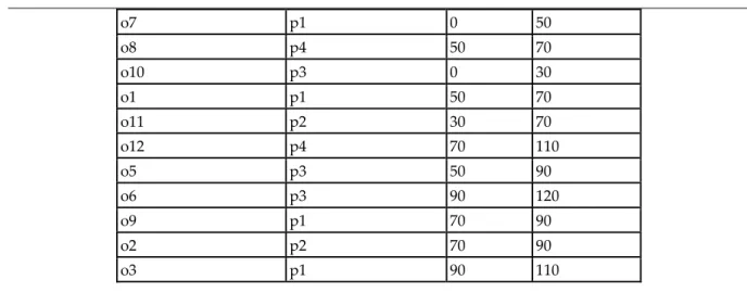
The output solution of the algorithm illustrated in (Table 6), shows the start and finish time for each operation, and the processor in which it runs the operation. In order to facilitate the solution, (Figure 5) presents how each operation in each job has started and finished with considering the max-load and ports for each processor. For example, job 2 started with o4 on p4 with a finishing time of 50-time units, then o5 of the same job started immediately on p3 at time 50 (the finishing time of o4) and finished on the start time of o6 of the same job with 90-time units in the same processor p3, then o6 finished at time 120-time units in the same processor. As we notice, the idle attribute shows how much each processor remained idle with a sum of 100-time units for all processors. For example, p2 remained idle after for 30-time units before working starting to work on o11. The operation load column represents the sum of operations load in the processor, such as p1 has a load of 80 units which is less than it is max-load.

Table 6. Output solution of 12 operations from the program

Operation Processor Start Finish

o4 p4 0 50

Processor Max Load Ports Load Remaning ports IDLE

P1 100 3 80 1 10 P2 150 5 40 3 60 P3 90 3 60 1 20 P4 120 3 70 0 10 Total 460 14 250 5 100 J3.o12=[70,110] J1.o2=[70,90] J1.o3=[90,110] J3.o11=[30,70] J2.o4 =[0,50] J2.o5=[50,90] J2.o6=[90,120] J3.o7=[0,50] J3.o8=[50,70] J3.o9=[70,90] J3.o10 =[0,30] J1.o1=[50,70] Operation

o7 p1 0 50 o8 p4 50 70 o10 p3 0 30 o1 p1 50 70 o11 p2 30 70 o12 p4 70 110 o5 p3 50 90 o6 p3 90 120 o9 p1 70 90 o2 p2 70 90 o3 p1 90 110

5.2. Scheduling 24 operations

The genetic algorithm implemented in this section to solve a problem consisting of 24 operations, 6 jobs, and 7 sensors, which should be scheduled in 7 processors with a sum of max load of 1070 units. The idle time for this problem must be 360-time units and the lowest makespan must be 160-time units based on the longest job path that is job 4.

We considered the initial population as 200 chromosomes and ran the algorithm on 1000 generations. ( Table 7) shows the results of our proposed GA and provides information from the program output about the

schedule of jobs for each operation's start and finish time. For example, operation 4 started on processor 4 at time 0 and finished at 50. Then operation 5 started on processor 2 at time 50 and finished at 90, etc.

Table 7. Output solution of 24 operations from the program

Operation Processor Start Finish

o4 p4 0 50 o21 p2 0 40 o1 p1 0 20 o13 p5 0 50 o5 p2 50 90 o18 p5 50 80 o17 p3 0 30 o15 p2 90 130 o22 p1 40 70 o10 p7 0 30 o2 p3 30 50 o7 p6 0 50 o3 p7 50 70 o14 p4 50 90 o23 p6 70 90 o19 p1 80 120 o11 p5 80 120 o12 p4 120 160 o9 p2 130 150 o24 p5 120 130

o8 p6 90 110

o6 p7 90 120

o16 p7 130 160

o20 p3 120 140

The Gantt chart of the route of the operation is shown in (Figure 6). We can see the lowest makespan by following job four operations marked in yellow. the job starts from operation 13 at start time zero and finishes at 50 on processor 5, then operation 14 starts at time 50 ( the finish time of operation 13) and finishes at 90 on processor 4, then operation 15 starts at time 90 (the finish time of operation 14) and finishes at time 130 on processor 2. Finally, operation 16 which is the last operation of job four starts at time 130 and finishes at 160 that is the lowest makespan of the GA. Also, job 3 has the same makespan 160 but it has been queued 50-time units after processing operation 10, which is not considered to be the lowest makespan explained in section 4.1.6.

Figure 6. Gantt chart of the optimal solution for scheduling 24 operations

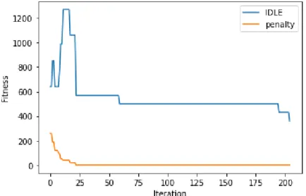
The best result was obtained after 204 epochs that caused the algorithm to stop due to the termination criteria. The penalty function dropped to zero after 24 epochs, which shows how the algorithm was penalized until it learned how to schedule the operations. The idle time was changing in irregular shape because it was exchanging depending on the value resulting from the penalty function. The idle time started decreasing immediately when the penalty has reached zero (Figure 7). The program prioritizes the penalty value until it reaches zero, then it will look at the optimal idle time.

Figure 7. The evolution process of idle time and the penalty function of running 24 operations

Processor Max Load ports load Remaning portsIDLE

P1 100 3 90 0 70 P2 150 5 130 1 20 P3 90 3 40 1 90 P4 120 3 110 0 30 P5 J6.O24 = [120 - 130] 300 5 100 1 30 P6 150 5 130 3 70 P7 160 5 50 1 50 Total 1070 29 650 7 360 J3.O11= [80 - 120] J3.O12 = [120 - 160] J6.O21 = [0 - 40] J2.O4=[0-50] J2.O5 = [50 - 90] J2.O6 = [90 - 120] J3.O8 = [90 - 110] J4.O16 = [130 - 160] J6.O23 = [70 - 90] J5.O17=[0-30]

J1.O1 = [0 - 20] J6.O22 = [40 -70] J5.O19 = [80 - 120]

J3.O7=[0-50] J4.O14 = [50- 90] J3.O9 = [130 - 150] J5.O20 = [120 - 140] J1.O2 = [30 -50] J1.O3 = [50 - 70] Operation J4.O13=[0-50] J3.O10=[0 - 30] J5.O18 = [50 - 80] J4.O15 = [90 - 130]

6. Discussion

When working with unsupervised learning, in general, a complete understanding of the problem plays a major role in the quality of work. Moreover, it gives a clear view of what needed to be done to complete the project. In this thesis, the main goal was to investigate a solution for a scheduling problem that is linked to a smart vertical farm for scheduling the farm activities to control the farm remotely. Thus, a clear goal from the start was to create a suitable data capabilities on scheduling operations in processors to deploy on the developed model. Creating good input data would simplify developing a good model. The most fitting data in this regard was divided onto three main categories to facilitate the complexity of the problem.

The JSP is an NP-hard problem, which means there is no proper method to solve the problem. And each problem has a different scenario and representation. The suitable data was created concerning this problem is divided into; 1) operations dataset, 2) tasks dataset, 3) processor dataset. Our assumptions were based on developing tasks data and linking them to appropriate jobs for every set of tasks. The processors and their properties were created in new dataset separately because it does not have a direct relation with the tasks, therefor, processors represent the machine's environment that runs the tasks. Fortunately, many studies have used this hypothesis to prove the correctness of the created data to represent the problem as required for real-world applications [13], [18].

The first part of section 6 holds the results of scheduling 12 operations in 4 processors in section 5.1. This experiment was oriented toward finding the optimal solution on small a small dataset. The goal of the experiment was to test the speed and efficiency of the algorithm. It was by luck to find the optimal solution after 27 epochs only. Some other results were obtained after 500 epochs and were not optimal. Due to the pure randomness of the algorithm, we obtained the optimal result in a very short time. But it does not guarantee that we can get this optimal result after every 27 epochs to schedule 12 operations.

The second part of section 6 holds the results of all 24 operations created in the dataset to be scheduled on 7 processors. The desired output has resulted after 204 epochs. The algorithm performed slower due to the larger data input used in the algorithm to obtain the result after approximately 4 hours. As we noticed, we obtained the optimal results when applying the algorithm on a larger dataset with a minimum makespan of 160-time units. This proves how powerful the designed solution to solve the proposed JSP.

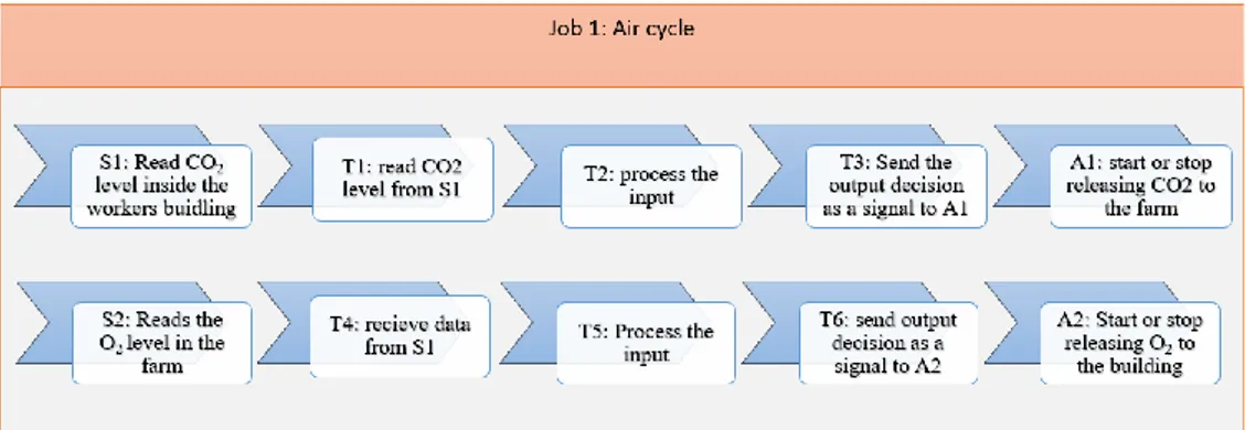
Figure 8. Air cycling job example on the farm

The direct connection between JSP and the VF is that each growth factor in the farm represents a job. Some of those jobs comprise another set of jobs. We represent the deployment of the JSP in the farm in (figure 8). The air recycling job is responsible for releasing CO2 from the workers building onto the vegetations cabins and releasing the O2 that produced from the plants onto the workers building by air conditioners. The job contains two major sensors. The first sensor S1 is responsible to read the CO2 level inside the workers building to send this data to the first task T1. Then, processing the inputs to make a decision in T2. After that, T3 sends the output decision to the actuator A1 that is responsible for releasing the CO2 to the farm. The second sensor S2 is responsible for the opposite, it reads the O2 level in the farm and sends it to the next task that is T4, Then, T5 process the input received from T4 to make a decision. Finally, the last task T6 sends the output decision as a signal to A2 that is responsible for releasing O2 to the workers building. This example illustrated a solution for controlling one of many growth factors on the farm. By applying the algorithm for controlling the farm, we reduce time, cost, and produce the finest quality of vegetables.

7. Conclusions

This study set out to develop an effective genetic algorithm for the job-shop scheduling problem to provide a systematic approach for controlling a smart vertical farm. The results of this research shown that the applied algorithm performs effectively to find the optimal solution of the problem. The relevance of vertical farming is clearly supported by the current findings of the research. These findings have significant implications for the understanding of how to apply the algorithm in the field of vertical farming.

A final research was designed to answer three research questions in particular. The definition and conclusions for each of the questions are as follow:

• RQ1: What is the suitable implementation of the EA technique to control food production until the next

harvest?

A limited number of previous studies suggested AI techniques applied to IVF. Through investigation and literature review studies into vertical farming, controlling food production line in the farm is a simulation of the optimal solution to the proposed job-shop scheduling problem. Our solution functions by combining and dividing the processes that the plant needs in the farm and applying the structure input to the algorithm. The algorithm then starts processing the input data and begins creating random solutions, taking into account the constraints in the problem.

• RQ2: How can we predict the time to next harvest?

The time to harvest any plant comes after providing all the important factors for the vegetation in terms of resources and time. Therefore, the harvest time of plants could be predicted in the farm by determining the required tasks and the time that the plants need and entering them into the algorithm that works to regulate the processes, which allows us to know when the next harvest time.

• RQ3: How could this EA technique enhance food productivity?

The process of improving plant productivity is carried out through organizing the agricultural processes that allow the farm to grow the plants in a controllable environment commensurate with plant life. By controlling the farm growth factors, there will be no waste of time and money because it will give the plants the exact required amount of the needed factor without increasing or decreasing, thus producing a better quality of food.

For future work, it will be interesting to investigate the following issues:

• Test the algorithm on a larger size data in order to see it is performance when dealing with large inputs. • Let the algorithm choose the number of processors by itself without instructing it, regarding the sum of

operations size.

References

[1] M. Al-Chalabi, “Vertical farming: Skyscraper sustainability?”. Sustainable Cities and Society, vol. 18, 2015, pp. 74-77.

[2] V. Lakshmi, and J. Corbett, “How artificial intelligence improves agricultural productivity and sustainability: A global thematic analysis”. In Proc. of the 53rd Hawaii International Conference on System Sciences, jan. 2020

[3] M. R. Garey, D. S. Johnson, and R. Sethi, “The complexity of flowshop and jobshop scheduling”. Mathematics of operations research, vol 1, no 2, 1976, pp. 117-129.

[4] R. L. Graham, “Bounds for certain multiprocessing anomalies”. Bell system technical journal, vol 45, no 9, 1966, pp. 1563-1581.

[5] P. Brucker, “The job-shop problem: Old and new challenges”. In Proc. of the 3rd Multidisciplinary International Conference on Scheduling: Theory and Applications (MISTA) aug. 2007, pp. 15-22. [6] M. SharathKumar, E. Heuvelink, and L. F. Marcelis, “Vertical farming: Moving from genetic to

environmental modification”. Trends in plant science, vol 25, no 8, 2020, pp. 724-727.

[7] K. Benke, and B. Tomkins, ”Future food-production systems: vertical farming and controlled-environment agriculture”. Sustainability: Science, Practice and Policy, vol. 13, no. 1, 2017, pp. 13-26. [8] M. I. H. B. Ismail and N. M. Thamrin, “IoT implementation for indoor vertical farming watering system”.

In 2017 International Conference on Electrical, Electronics and System Engineering (ICEESE), pp. 89-94.

[9] Z. Ghahramani, “Unsupervised learning”. In Summer School on Machine Learning. Springer, Berlin, Heidelberg, feb. 2003, pp. 72-112.

[10] T. Back, “Evolutionary algorithms in theory and practice: evolution strategies, evolutionary programming, genetic algorithms”. Oxford university press, 1996.

[11] H. Wilde, V. Knight, and J. Gillard, “Evolutionary dataset optimisation: learning algorithm quality through evolution,” Applied Intelligence, vol. 50, no. 4, 2019, pp. 1172–1191.

[12] D. Whitley, “A genetic algorithm tutorial,” Statistics and Computing, vol. 4, no. 2, 1994.

[13] S. Noor, M. I. Lali, and M. S. Nawaz,”Solving job shop scheduling problem with genetic algorithm”. Science International, vol. 27, no. 4, 2015.

[14] L. Sun, X. Cheng, and Y. Liang, “Solving Job Shop Scheduling Problem Using Genetic Algorithm with Penalty Function,” International Journal of Intelligent Information Processing, vol. 1, no. 2, 2010, pp. 65–77.

[15] Y. Tsujimura, M. Gen, and E. Kubota, “Solving Job-shop Scheduling Problem with Fuzzy Processing Time Using Genetic Algorithm,” Journal of Japan Society for Fuzzy Theory and Systems, vol. 7, no. 5, 1995, pp. 1073–1083.

[16] F. Pezzella, G. Morganti, and G. Ciaschetti, “A genetic algorithm for the Flexible Job-shop Scheduling Problem,” Computers & Operations Research, vol. 35, no. 10, 2008, pp. 3202–3212.

[17] G. Zhang, L. Gao, and Y. Shi, “An effective genetic algorithm for the flexible job-shop scheduling problem,” Expert Systems with Applications, vol. 38, no. 4, 2011, pp. 3563–3573.

[18] S. Meeran and M. S. Morshed, “A hybrid genetic tabu search algorithm for solving job shop scheduling problems: a case study,” Journal of Intelligent Manufacturing, vol. 23, no. 4, 2012, pp. 1063–1078.

Appendix: Source code for testing the GA

_o_operation = _raw_pop.at[_o, 'Operation']

_o_task = _df_operation['Task'].loc[_df_operation['Operation'] == _o_operation].reset_index(drop=True)[0] _o_task_load = _df_tasks['Load'].loc[_df_tasks['Task'] == _o_task].reset_index(drop=True)[0]

_o_sensor =_df_operation['Sensor'].loc[_df_operation['Operation'] == _raw_pop['Operation'][_o]].reset_index(drop=True)[0]

_o_process_max_load =_processing_units['Maxload'].loc[_processing_units['Processor'] == _raw_pop['Processor'][_o]].reset_index(drop=True)[0] _o_process_max_port = _processing_units['Ports'].loc[_processing_units['Processor'] == _raw_pop['Processor'][_o]].reset_index(drop=True)[0] if(_Processer_ports.count([_raw_pop['Processor'][_o] , _o_sensor]) >0):

_processing_units['Maxload'].loc[_processing_units['Processor'] == _raw_pop['Processor'][_o]] = _o_process_max_load - _o_task_load

else:

_processing_units['Maxload'].loc[_processing_units['Processor'] == _raw_pop['Processor'][_o]] = _o_process_max_load - _o_task_load _processing_units['Ports'].loc[_processing_units['Processor'] == _raw_pop['Processor'][_o]] -= 1

_Processer_ports.append([_raw_pop['Processor'][_o], _o_sensor])

available_penalty += _processing_units['Maxload'].loc[_processing_units['Maxload']<0].sum() return available_penalty

Listing 1: The availability penalty function

def calculate_penalty(_chromosome): _raw = _chromosome.copy() _penalty = 0

for _o_index in range(len(_raw)):

_operation = _raw['Operation'][_o_index]

_operation_dep = _df_operation['dep'].loc[_df_operation['Operation'] == _operation].reset_index(drop=True)[0] if _operation_dep != "s":

_operation_time_start = _raw['start'][_o_index]

_operation_dep_time_finish = _raw['finish'].loc[_raw['Operation'] == _operation_dep].reset_index(drop=True)[0] if _operation_time_start < _operation_dep_time_finish:

_penalty += int(_operation_dep_time_finish) - int(_operation_time_start)

return _penalty

Listing 2: The rescheduling penalty function

def fitness(population): _df_pop_fitness = population.copy() _df_fitness = [] for i in range(len(_df_pop_fitness)): _df_pop_fitness[i]['start'] = 0 _df_pop_fitness[i]['finish'] = 0

for _o_index in range(len(_df_pop_fitness[i])):

_processor = _df_pop_fitness[i]['Processor'][_o_index] _operation = _df_pop_fitness[i]['Operation'][_o_index]

_operation_dep = _df_operation['dep'].loc[_df_operation['Operation'] == _operation].reset_index(drop=True)[0]

_o_exec_t = _df_tasks['Exec'].loc[_df_tasks['Task'].isin( _df_operation['Task'].loc[_df_operation['Operation'] == _operation ])].reset_in dex(drop=True)[0]

_last_o_finish_in_processor = _df_pop_fitness[i]['finish'].loc[_df_pop_fitness[i]['Processor'] == _processor].max() _o_start =0

if(_operation_dep == "s"):

else:

_o_dep_finish = _df_pop_fitness[i]['finish'].loc[_df_pop_fitness[i]['Operation'] == _operation_dep].reset_index(drop=True)[0] _o_start = max(_last_o_finish_in_processor, _o_dep_finish)

_o_finish = _o_start + _o_exec_t

_df_pop_fitness[i].at[_o_index,'start'] = _o_start _df_pop_fitness[i].at[_o_index, 'finish'] = _o_finish

_make_span = _df_pop_fitness[i]['finish'].max() _dt_processors = _df_components.copy() _dt_processors['IDLE'] = _make_span for _p in range(len(_dt_processors)):

_o_in_processor = _df_pop_fitness[i].loc[_df_pop_fitness[i]['Processor'] == _dt_processors['Processor'][_p]] _o_in_processor['Operation_time'] = _o_in_processor['finish'] - _o_in_processor['start']

_dt_processors.at[_p, 'IDLE'] = _dt_processors['IDLE'][_p] - _o_in_processor['Operation_time'].sum()

_available_pen = GA.availability_penalty(_df_pop_fitness[i])* -1

_reschedule_penalty = GA.calculate_penalty(_df_pop_fitness[i])

_df_fitness.append([_available_pen, _reschedule_penalty, _dt_processors['IDLE'].sum(), _make_span])

_df_fitness = pd.DataFrame(_df_fitness, columns=['Availability_Penalty','Rescheduling_Penalty','IDLE', 'Make_span']) return _df_fitness

Listing 3: The fitness function

def prents_selection(_population, _fitness, _num_parents): _df_pop = _population

_selected_parents = []

_df_fitness_sort = _fitness.sort_values(by=['Availability_Penalty','Rescheduling_Penalty','IDLE', 'Make_span']).reset_index() for _parent in range (_num_parents):

_selected_parents.append(_df_pop[_df_fitness_sort['index'][_parent]]) return _selected_parents

Listing 4: Parents selection function

def crossover(parents): _df_pop = parents.copy() _df_new_parents =[] for i in range(len(_df_pop)): p1 = _df_pop[i] p2 = _df_pop[(i+1) % len(_df_pop)]

_index1 = r.randint(int(len(_df_operation)/2), len(p1)-1) _index2 = r.randint(int(len(_df_operation)/2), len(p1)-1) if _index1>_index2:

_val = _index2 _index2 = _index1 _index1=_val

_part = p1[_index1: _index2]

p2 = p2[~p2['Operation'].isin(_part['Operation'])].reset_index(drop=True) p2 = p2.append(_part).reset_index(drop=True)

r.shuffle(p2['Processor']) _df_new_parents.append(p2)

return _df_new_parents

def mutation(offspring_crossover):

_mutation_pop = offspring_crossover.copy() _mutation_crossover = []

for i in range(len(_mutation_pop)):

_index_i = r.randint(0, len(_mutation_pop[i]) -1) _index_x = r.randint(0, len(_mutation_pop[i]) -1) _i_row = _mutation_pop[i].loc[_index_i] _x_row = _mutation_pop[i].loc[_index_x] r.shuffle(_mutation_pop[i]['Processor']) if np.random.uniform(0,1) < 0.5: if _index_i > _index_x: _val = _index_i _index_i = _index_x _index_x = _val list_index = _mutation_pop[i].index.tolist() inverted_index = list_index[_index_i:_index_x] inverted_index.reverse() list_index[_index_i:_index_x] = inverted_index _mutation_pop[i].index = list_index _mutation_crossover.append(_mutation_pop[i]) return _mutation_crossover

Listing 6: Mutation operator function

_num_POPULATION = 200

_num_parents = 100

GENERATIONS = 1000

_df_population = []

for pop in range (_num_POPULATION):

_row_pop = _df_operation['Operation'].copy() r.shuffle(_row_pop)

_row = _df_components['Processor'].iloc[np.random.randint(0, len(_df_components), _row_pop.shape[0])].reset_index(drop=True) _row_pop = pd.concat([_row_pop, _row.rename("Processor")], axis=1)

_df_population.append(_row_pop) _generation_history =[]

_generation_fitnness_history =[] _generation_penalty_history = []

_generation_availability_penalty_history = []

for gene in range(GENERATIONS):

_pop_fitness = GA.fitness(_df_population.copy())

_pop_fitness_sort = _pop_fitness.sort_values(by=['Availability_Penalty','Rescheduling_Penalty','IDLE', 'Make_span']).reset_index()

print(f"Best result: {gene} : IDLE= { _pop_fitness_sort['IDLE'][0]} ,Availability_Penalty = {_pop_fitness_sort['Availability_Penalty'][0]} ,Resc heduling_Penalty = {_pop_fitness_sort['Rescheduling_Penalty'][0]} , MakeSpan = {_pop_fitness_sort['Make_span'][0]}")

_generation_history.append(gene)

_generation_fitnness_history.append(_pop_fitness_sort['IDLE'][0])

_generation_penalty_history.append(_pop_fitness_sort['Rescheduling_Penalty'][0])

_generation_availability_penalty_history.append(_pop_fitness_sort['Availability_Penalty'][0]) _pop_selected_parents = GA.prents_selection(_df_population,_pop_fitness, _num_parents)

if(int(_pop_fitness_sort['Availability_Penalty'][0])== 0and int(_pop_fitness_sort['Rescheduling_Penalty'][0])== 0and int(_pop_fitness_sort['Mak e_span'][0]) == _minimum_makespan): break _pop_crossover = GA.crossover(_pop_selected_parents) _pop_mutation = GA.mutation(_pop_crossover) _new_population = _pop_mutation

_new_population.append(_pop_selected_parents[i]) _random_pop_index = [i for i in range(_num_POPULATION)][:] r.shuffle(_random_pop_index)

for i in range(50):

_new_population.append(_df_population[ _random_pop_index[i]]) _df_population = _new_population

print(f"Best solution:", _pop_selected_parents[0])