DEGREE PROJECT, IN COMPUTATIONAL CHEMISTRY , FIRST LEVEL
STOCKHOLM, SWEDEN 2015
Interaction potential energy between
finite rectangular cellulose nanofibrils
NONLINEAR POISSON-BOLTZMANN THEORY
KARAN AHMADZADEH
Abstract
Thermodynamically, native cellulose nano fibrils are more stable in an aggregated state. The aggregated state is however not useful from a material development perspective. Therefore much research has been done to stabilize the dispersal of the fibrils. One method to overcome this instability is by surface substitution of the O6 hydroxyl group with carboxylate groups, to make highly charged fibrils in aqueous solutions. It is therefore of much interest to understand the interaction of highly charged fibrils in aqueous solutions. In this study, we aim to model the interaction potential energy between native and surface modified cellulose nanofibrils in order to understand under what conditions the contribution from the dipole interactions can be neglected. To achieve this we propose to use a continuum electrostatic approach, modeling the electrostatic interactions as a function of the fibrils relative dipole orientation, separation, surface charge as well as ionic strength of the solution, by means of using the Poisson-Boltzmann equation.
Our findings suggest that the highly charged cellulose nanofibrils cannot be modeled with the Poisson-Boltzmann equation, as the high surface charge itself causes the key assumptions of the Boltzmann statistic description of the free ion distribution to break down in the diffuse double layer. Our results are therefore inconclusive and the conclusion to be drawn from this entire study is that the interaction potential energy between highly charged surfaces must be modeled with a more advanced description of the diffuse double layer. To this end we derive a new relation that approximates the theoretical limit for the surface potential in term of bulk parameters.
Contents
... 1
1. Introduction ... 1
1.2 Purpose ... 2
1.1 The Poisson-Boltzmann equation ... 2
1.3 Theory - Electrostatic potential for finite rectangular fibrils ... 3
Region 𝜴𝟏- The dispersed fibril ... 3
Region 𝜴𝟐- Ion exclusion layer ... 3
Region 𝜴𝟑- Solvent ... 3 Boundary’s ... 4 2. Method ... 5 2.1 The fibrils ... 5 2.2 Orientation ... 5 2.3 Partial Charges ... 6
2.4 Determination of the interaction potential ... 6
2.5 The Poisson-Boltzmann equation ... 7
2.6 The Poisson equation ... 7
2.7 Additional remarks ... 7
3. Results and Discussion ... 8
3.1 Debye length ... 8
3.2 Concavity of potential functions ... 10
3.3 Cogency of data ... 11
3.4 Nanofibrils ... 12
3.5 Surface charge density ... 13
3.6 Surface potential – Graham’s equation ... 13
3.7 Free ion charge density ... 13
3.8 Number of counter ions at surface ... 14
3.9 Inter ion separation... 14
3.10 Theoretical limit ... 15
3.11 Conclusion ... 17
Appendix A – Electrostatic force ... 19
Force field from distribution of point charges ... 19
Appendix B – Divergence ... 20
Appendix C – Gauss's theorem and law of electrostatics ... 22
Relating force and energy ... 24
Appendix E – Columbus law ... 25
Appendix F – The Poisson equation ... 26
Appendix F-2 – The Laplacian of 𝝍 ... 26
Appendix F-3 – Solution to Poisson’s equation ... 27
Appendix G – Electrostatic double layer ... 29
Appendix H Flux density and diffusion ... 30
Convective flux density ... 30
Appendix H-1– The formation of the charge distribution ... 33
Appendix I –Statistical description of the free ions ... 37
Appendix J – The Poisson-Boltzmann equation ... 47
Appendix K – Double layer from charged surfaces ... 48
Appendix L – Interaction potential between two surfaces. ... 50
Appendix - M Assumptions behind the DLVO theory ... 54
Appendix N – Linear and nonlinear Poisson-Boltzmann equation. ... 54
Appendix O – Determination of surface potential ... 56
1
1. Introduction
Colloids are classified as homogenous mixtures, where particles of diameters between 1 to 1000 nm are suspended in solution. Native cellulose can be processed to be in the form of nanocrystal (CNC) particles, only a few nanometers wide and approximately 150 nm long. These particles are known to have low colloidal stability. [4] Colloidal stability refers to the resistance of the colloidal particles against aggregation.
Figure: Aggregated state (left) with less surface area exposed to the liquid. Dispersed phase (right) [4]
For solid colloids dispersing from their aggregated state, the change in free energy is given by the expression
𝑑𝐺 = 𝑉𝑑𝑝 − 𝑆𝑑𝑇 + 𝛴𝜇𝑑𝑛 + 𝛾𝑑𝐴 + 𝑇𝑑𝑆 Where the term 𝛾𝑑𝐴is known as the work of adhesion. [1] Work of adhesion is defined as the work needed to separate two
surfaces by working against the forces at the interfaces in order to disperse them completely. [2] For a reversible dispersion 𝑑𝑆 = 0 with constant temperature 𝑑𝑇 = 0, composition 𝑑𝑛 = 0, and pressure 𝑑𝑃 = 0. The free energy of this process only
depends on the surface energy 𝛾 and the change in area 𝑑𝐴 𝑑𝐺 = 𝛾𝑑𝐴 It follows that if 𝑑𝐴 > 0 Then 𝑑𝐺 > 0.
As dispersion from aggregates causes an increase in area 𝑑𝐴 > 0, and all processes move towards lower free energy, it is apparent why the aggregate is more thermodynamically stable. [1]
Dispersed cellulose fibrils: The cellulose fibrils used in this work are composed of 16 chains made of 20 glucose monosaccharides in a rectangular configuration with a height of 4 chains and a width of four chains.
The aggregated form of cellulose is not useful from a material development perspective. Therefore much research has been done in altering the fibrils to stabilize the dispersion. One method to stabilize the dispersion is to increase the surface charge of the fibrils, by surface substitution, and thus obtain electrostatically stable colloids. The electrostatic stabilization can be
understood in terms of the Derjaugin, Landau, Verwey and Overbeek (DLVO) theory. [20] The DLVO theory describes the aggregation of dispersed particles as an interplay between Van der Waals forces and electrostatic double layer forces.
∇𝜓𝑖𝑛𝑡𝑒𝑟𝑎𝑐𝑡𝑖𝑜𝑛 = ∇𝜓𝑣𝑎𝑛+ ∇𝜓𝑒𝑙𝑒𝑐𝑡𝑟𝑜𝑠𝑡𝑎𝑡𝑖𝑐 At short range the van der Waals forces dominate and according to Lipchitz theory [3] the Van der Waals force is always attractive for similar materials and thus
2 favors aggregations. The electrostatic
double layer force between like charged particles creates an energy barrier that prevents the dispersed particles from aggregating again and thus favors, or stabilizes the dispersed state, see figure below. [1]
Interaction energy between charged colloids.Intermolecular and Surface Forces by Jacob N. Israelachvili. [1]
The work of adhesion discussed earlier is the work needed to separate two surfaces against the van der Waals force at short distances, thus it is apparent why without an electrostatic repulsive force the aggregated state is more thermodynamically stable. The strength of the Van der Waals forces however reduces rapidly with distance, and the much longer range electrostatic force dominates. [5]
At intermediate distances it is therefore more computationally appropriate to analyze the behavior of the dispersed phase in terms of the electrostatic forces alone, which is the focus of the present paper.
1.2 Purpose
In order to disperse the fibrils, surface modifications such as TEMPO oxidation have been performed where the surface hydroxyl groups are substituted with carboxylate groups, making the surface highly charged. [24] The purpose of this study is to model the interaction between neutral cellulose fibrils and TEMPO oxidized
Cellulose fibrils. Once the dispersed cellulose has been attained, it is of interest to investigate how the dispersed fibrils orient themselves in the suspension, as this permits better control of the final material structure. In this paper we look at two dispersed cellulose nanofibrils, in a
monovalent ionic solution. The orientation of the dispersed fibrils will be analyzed electrostatically, with the nonlinear Poisson-Boltzmann equation. In particular we will study how the relative orientation of the fibrils affect their interaction potential. The influence of the ionic
strength, radial distance and surface charge on orientation will be explored.
Furthermore the relative strength of the dipole and electrostatic repulsion will be determined.
1.1 The Poisson-Boltzmann equation
The electrostatic double layer interaction 𝜓𝑒𝑙𝑒𝑐𝑡𝑟𝑜𝑠𝑡𝑎𝑡𝑖𝑐 between the dispersed fibrils
can be computed with the nonlinear Poisson-Boltzmann, PBE equation, see Appendix J, whose solution 𝜓(𝑥, 𝑦, 𝑧) gives the potential due to the charges that make up the cellulose fibrils and the ionic species in the environment. To obtain the
interaction potential energy between two dispersed fibrils, the PBE can theoretically first be solved for a system comprised of two fibrils at a set radial distance, ionic concentration and surface charge. The PBE is then solved for an isolated cellulose fibril, in the same environment and surface charge. The difference between these two quantities is a function
𝜓𝑖𝑛𝑡𝑒𝑟𝑎𝑐𝑡𝑖𝑛 = 𝜓𝑡𝑤𝑜𝑓𝑖𝑟𝑏𝑟𝑖𝑙𝑠− 2𝜓𝑖𝑠𝑜𝑙𝑎𝑡𝑒𝑑 With the property
lim
3 Where
x is the distance between the colloids R is some finite distance much larger than
the Debye length 𝜅−1
and is known as the electrostatic interaction
potential 𝜓𝑒𝑙𝑒𝑐𝑡𝑟𝑜𝑠𝑡𝑎𝑡𝑖𝑐. By comparing the
𝜓𝑒𝑙𝑒𝑐𝑡𝑟𝑜𝑠𝑡𝑎𝑡𝑖𝑐 for different orientations, the naturally adopted orientation for two fibrils can determined as the net force acting on the fibrils is always directed in the direction of the negative potential gradient, and thus the direction of maximum decrease of potential energy.
𝐹⃗ = −𝑞∇ψelectrostatic
See Appendix D.
1.3 Theory - Electrostatic potential for finite rectangular fibrils
Consider an isolated fibril in solution, since the surface is charged an ion-exclusion layer will form around it, whose domain will be
denoted 𝛺2. The fibril itself will belong to
domain 𝛺1 and the solvent will be 𝛺3. We
treat the solvent and exclusion layer as continuous medium with a certain dielectric constant, disregarding the particle features of the solvent and the ions residing in it, we model the ions as a continues charge distribution, see Appendix I-J for more information.
The charge density and electric potential is related by the Poisson equation. To obtain the potential distribution around the fibril, we apply Poisson equation to every region
separately. That is, for 𝛺𝑘
𝛻2𝜓(𝑟)𝑘 = − 𝜌(𝑟)𝑘
𝜖𝑘
Region 𝜴𝟏- The dispersed fibril
As we do not model electrons, we assign
every particle making up the fibril, a partial
charge. In domain 𝛺1 the potential made
by these partial charges is given by the expression: 𝜓1(𝑟) = ∑ 𝑞𝑖 4𝜋𝜖1 1 |𝑟 − 𝑟𝑖| 𝑛 𝑖=1
Which is simply the Columbic potential.
Where 𝑟𝑖 is the position of the i:th charge,
and n is the total number of charges in
region 𝛺1. Applying Green's function for the
Laplacian we obtain [6]. 𝛻2𝛹 1(𝑟) = ∑ −4𝜋𝑞𝑖 𝜖1 𝛿(𝑟 − 𝑟𝑖) 𝑛 𝑖=1 where 𝛿 𝑖𝑠 𝑡ℎ𝑒 𝑑𝑖𝑟𝑎𝑐 𝑑𝑒𝑙𝑡𝑎 𝑓𝑢𝑛𝑐𝑡𝑖𝑜𝑛 𝛿(𝑟 − 𝑟𝑖) = { ∞ 𝑓𝑜𝑟 𝑟 = 𝑟𝑖 0 𝑓𝑜𝑟 𝑟 ≠ 𝑟𝑖
Region 𝜴𝟐- Ion exclusion layer
In the ion exclusion layer there are no charges, therefore by gauss's law, see Appendix C.
∇𝜓22= 0
Region 𝜴𝟑- Solvent
The concentration at any point (𝑥, 𝑦, 𝑧) depends on the energy needed to bring all the ions there as discussed in Appendix J, and thus the charge density is in general given by the expression
𝜌(𝑥, 𝑦, 𝑧) = 𝑒(∑ 𝑐0𝑖𝑒−𝜓(𝑥,𝑦,𝑧) 𝑞𝑖𝑒/𝑘𝑏𝑇 𝑁 𝑖=1 − ∑ 𝑐0𝑗𝑒𝜓(𝑥,𝑦,𝑧) 𝑞𝑗𝑒/𝑘𝑏𝑇) 𝑀 𝑗=1 Where 𝜌 is the charge density e is the electron charge
4
𝜓 is the electrostatic potential 𝑞𝑖is the valence
𝑘𝐵is the Boltzmann constant
T is the absolute temperature
Assuming there is only one variety of positive and negative ions in the solution and that the bulk concentration of both are
equal (𝑐0−= 𝑐0+) the summation may be
dropped and we obtain the expression
𝜌(𝑥, 𝑦, 𝑧) = 𝑒(𝑐0𝑒
−𝜓(𝑥,𝑦,𝑧) 𝑒𝑞𝑘
𝑏𝑇 − 𝑐0𝑒
𝜓(𝑥,𝑦,𝑧)𝑒 𝑞 𝑘𝑏𝑇 )
Noting that the hyperbolic function of sine is
𝑠𝑖𝑛ℎ(𝑥) = 𝑒
𝑥− 𝑒−𝑥
2
and so the potential due to the ionic distribution is given by the expression
𝛻2𝜓(𝑥, 𝑦, 𝑧) =2𝑒𝑐0 𝜖3
𝑠𝑖𝑛ℎ (𝜓(𝑥, 𝑦, 𝑧) 𝑞𝑖 𝑘𝐵𝑇
)
To get an expression for the combined regions we introduce two functions
𝜖(𝑥, 𝑦, 𝑧) = { 𝜖1 𝑖𝑓 𝑟 ∈ Ω1
𝜖2= 𝜖3 𝑖𝑓 𝑟 ∈ Ω2 𝑜𝑟 𝑟 ∈ Ω3
𝜅(𝑥, 𝑦, 𝑧) = {0 𝑖𝑓 𝑟 ∈ Ω1 𝑜𝑟 𝑟 ∈ Ω2 √𝜖3𝑘 𝑖𝑓 𝑟 ∈ Ω3
Furthermore to ensure that the solution 𝜓(𝑥, 𝑦, 𝑧) is continues on the boundary
regions between Ω1, Ω2 and Ω3 we require
that the function takes the same value on the boundary [6]
𝜓𝑘(𝑥, 𝑦, 𝑧) = 𝜓𝑘+1(𝑥, 𝑦, 𝑧)
Boundary’s
Elliptic partial differential equations, are time independent, and thus describe steady
state phenomenon, that only depend on spatial variables. In this case the variation of the potential in space. Time independent problems such as these are usually solved for a certain kind of boundary conditions, known as Dirichlet boundary conditions. The types of boundary condition problems we are concerned with are the interior and exterior Dirichlet problems. At the
boundary of the regions we require that the potential takes the value of the analytical solutions of the Debye-Hückel model.
Figure: Interior Dirichlet boundary condition. The PDE holds inside the domain, and the solution is specified on the boundary of the domain 𝑑Ω
Figure: Exterior Dirichlet boundary condition. The PDE holds outside the domain, and the solution is specified on the boundary of the domain 𝑑Ω
5 𝜓(𝑥, 𝑦, 𝑧) = 𝜓(𝑥, 𝑦, 𝑧)𝐷𝑒𝑏𝑦𝑒−Hückel
For
(𝑥, 𝑦, 𝑧) ∈ 𝑑Ω
Then the full nonlinear Poisson-Boltzmann equation takes the form
−𝛻(𝜖(𝑥, 𝑦, 𝑧)𝛻𝜓(𝑥, 𝑦, 𝑧)) + 𝜅2(𝑘𝐵𝑇 𝑧𝑒) 𝑠𝑖𝑛ℎ ( 𝑞𝑖𝑒𝜓(𝑥, 𝑦, 𝑧) 𝑘𝐵𝑇 ) = 4𝜋 ∑ 𝑞𝑖𝛿((𝑥, 𝑦, 𝑧) − (𝑥𝑖,𝑦𝑖,𝑧𝑖)) 𝑛 𝑖=1 Where
𝜓 is the electrostatic potential
𝜅 𝑖𝑠 𝑡ℎ𝑒 𝑖𝑛𝑣𝑒𝑟𝑠𝑒 𝐷𝑒𝑏𝑦𝑒 𝑙𝑒𝑛𝑔𝑡ℎ 𝑓𝑢𝑛𝑐𝑡𝑖𝑜𝑛 𝑑𝑒𝑓𝑖𝑒𝑛𝑑 𝑎𝑏𝑜𝑣𝑒. 𝑞𝑖 is the valiancy of the ions
𝑘𝐵is the Boltzmann constant 𝑇 is the absolute temperature in kelvin 𝜖 is the dielectric constant function defined above
𝑒 is the electron charge
2. Method
In this project the interaction potential energy was modeled using computer simulations. The software package APBS solves the nonlinear Poisson-Boltzmann equation numerically with the finite
element method as is described in detail in the paper: The Poisson-Boltzmann Equation, Analysis and Multilevel Numerical Solution, M. J. Holst. [6]
The exact procedure and settings used are outlined in Appendix P.
2.1 The fibrils
The Cellulose fibrils modeled are estimated to have dimensions of roughly 2.5x2.5x10 nm and are composed of 20
monosaccharaide subunits (length).
Figure: Dimensions of fibrils that we model. Rough estimate.
Of the 20 monosaccharide that comprise the fibril length, half have hydroxyl groups pointing in to the bulk, which don’t contribute to the interaction.
Figure: Cellulose polymer illustrating that the O6 hydroxyl groups alternate in and out of the bulk. [2]
2.2 Orientation
In APBS, the dispersed cellulose was modeled for three different dipole orientations: perpendicular, parallel, and antiparallel.
Figure: Antiparallel orientation, green arrows represent the net dipole direction.
6 Figure: Parallel orientation, green arrows
represent the net dipole direction.
Figure: Perpendicular orientation, green arrows represent the net dipole direction.
For every orientation the three different surface charges were modeled. The radial distances considered were in the interval 2.5 nm –4.5 nm, from centers of mass. Furthermore three different ionic
concentrations for monovalent ions where used, namely c = 0, 0.01, 0.1M.
2.3 Partial Charges
In unmodified cellulose, the hydroxyl group oxygen has a partial charge of
𝛿𝑜𝑥𝑦𝑔𝑒𝑛= −0.65 ×1.60217657 × 10−19 𝐶𝑜𝑙𝑜𝑢𝑚𝑏𝑠 In each of the cases Q0,Q05, Q1 we increased the partial charge by −0.65 𝑒, where e is the electron charge. APBS calculates the net charge
by taking the number of charged groups on the surface times their charge and then removes the charge from the charges from within the fibril to get a net charge.
Case Partial charge oxygen 𝜹𝒐𝒙𝒚𝒈𝒆𝒏 Net charge fibril Q0 -0.65e 0 Q05 -1.15 e -70.0 e Q1 -1.65e -280e Table 1.
2.4 Determination of the interaction potential
Due limited time and computer resources and the consequent inaccuracy of the numerical method, the potentials did not go zero when we modeled the theoretical interaction potential energy
𝜓𝑖𝑛𝑡𝑒𝑟𝑎𝑐𝑡𝑖𝑛 = 𝜓𝑡𝑤𝑜𝑓𝑖𝑟𝑏𝑟𝑖𝑙𝑠− 2𝜓𝑖𝑠𝑜𝑙𝑎𝑡𝑒𝑑
Therefore we resorted to acquire the interaction potential energy by considering that the potential must go to zero at distances well beyond the Debye length, see Appendix K, we therefore corrected the error by take the non-zero value
𝜓𝑠𝑒𝑙𝑓= lim
𝑟→𝑅≫𝜅−1𝜓𝑡𝑤𝑜𝑓𝑖𝑏𝑟𝑖𝑙𝑠
As the energy of the isolated fibrils and we construct our interaction potential function as
𝜓𝑖𝑛𝑡𝑒𝑟𝑎𝑐𝑡𝑖𝑛= 𝜓𝑡𝑤𝑜𝑓𝑖𝑏𝑟𝑖𝑙𝑠−𝜓𝑠𝑒𝑙𝑓
In order to ensure that lim
7
2.5 The Poisson-Boltzmann equation
Since there was fluctuations in the data, we fit the data to a function of the form
𝑓 = 𝛼𝑒−𝑘𝑥
As this is predicted to be the form of the potential drop by DLVO theory based on the Poisson-Boltzmann equation for the
interaction potential between two surfaces.
𝜓 =64𝑐0𝑘𝐵𝑇 𝜅 tanh (
𝜓0𝑞
4𝑘𝐵𝑇
) 𝑒−𝜅𝑥
2.6 The Poisson equation
When there are no free ions in the solution, the Poisson-Boltzmann equation turns to the Poisson equation, which as was shown in appendix F predicts a linear potential drop, for these cases we fit to a linear polynomial of the form
𝑓 = 𝑎𝑥 + 𝑏
2.7 Additional remarks
The data from APBS is calculated with the distance taken from the center of mass of both fibrils. With respect to their centers of mass, they are never closer than 2.5 nm. In the DLVO theory, one considerers instead the radial distance from surface to surface. In order to correct for this in our model, we translated the curves.
𝑟𝑟 = 𝑟𝑐𝑒𝑛𝑡𝑒𝑟− 2𝛿
Where 𝑟𝑠 is the distance between the
surfaces and 𝛿 is the distance from the center of mass of each fibril to it’s own surface.
8
3. Results and Discussion
The method showed fundamental problems with calculating the potential energy. Firstly there was the issue of the potential
function coming out from APBS not abiding to the criteria
lim
𝑥→𝑅≫𝑘−1𝜓𝑖𝑛𝑡𝑒𝑟𝑎𝑐𝑡𝑖𝑛= 0 Meaning that the potential energy predicted by APBS was converging to a finite, yet none zero value for distances well beyond where the interaction should
sensibly go to zero. By taking the non-zero value
lim
𝑥→𝑅≫𝑘−1𝜓𝑖𝑛𝑡𝑒𝑟𝑎𝑐𝑡𝑖𝑛= 𝐾
As the self-energy of the fibrils, and then manipulating the data from APBS such that it goes to zero was not possible in a
satisfactory manner for all cases. Besides correcting so that the potential goes to zero, we also needed to make sure that the Debye lengths were correct after the translation.
3.1 Debye length
In appendix K, we showed that the Debye length is given by the expression
𝜅−1= 1
√2𝑐𝑖0𝑒2
𝜖𝜖0𝑘𝐵𝑇
Based on this we computed the Debye lengths independently of APBS for the 0.1M and 0.01M cases. 𝜅−1 = 1 √2 × 0.01 × 103× 6.022 × 1022× (1.6 × 10−19)2 78 × 8.85 × 10−12× 1.38 × 10−23× 298 𝜅−1= 3.03 𝑛𝑚 𝜅−1 = 1 √2 × 0.1 × 103× 6.022 × 1023× (1.6 × 10−19)2 78 × 8.85 × 10−12× 1.38 × 10−23× 298 𝜅−1= 0.95 𝑛𝑚
Concentration Debye length
0.01M 3.03 𝑛𝑚
0.1 M 0.95 𝑛𝑚
Table A
The Debye length for the 0.1M case was 0.9 nm and for a 0.01M solution 3nm. Meaning that the interaction potential energies should go to zero at around 6 nm and 16 nm respectively see figure A below, for further discussion see Appendix L.
Figure A: Interaction potential per unit area 𝜓 =64𝑐0𝑘𝐵𝑇
𝜅 tanh( 𝜓0𝑞 4𝑘𝐵𝑇)𝑒
−𝜅𝑥 for two surfaces in a monovalent symmetric salt solution, with concentrations 𝑐 = 0.1𝑀 (top figure) and 𝑐 = 0.01𝑀 (bottom figure). Illustrates that the Debye length is independent of surface potential and shows the characteristic interaction lengths.
Thus correcting the Debye lengths proved to be an impossible task with 298x298x298 grid points for the finite element method, as can be seen in figure 1,2 and 4.
9
Figure 1: Effect of charge on interaction potential for antiparallel fibrils. Data values fitted to the DLVO anticipated curve. 298x298x298 grid points for the finite element method
The fact that the Q0, antiparallel case in figure 1, does not match the electrostatic interaction potential predicted by DLVO theory, is however not surprising, as the Poisson-Boltzmann equation is a partial differential equation relating the interaction potential between charged particles. It is however surprising that the interaction potential for the Q0 surface fluctuates quite a bite around zero. This is hypothesized to be due to numerical error. It thus serves as a good indicator for the overall inaccuracy in all the calculations.
Figure 2: Effect of concentration on interaction potential for constant surface charge and antiparallel orientation. Data values fitted to exponential curve for Poisson-Boltzmann and linear for Poisson. 298x298x298 grid points for the finite element method
Looking at figure 2, we see that this method cannot model correctly or distinguish
between two antiparallel fibrils in 0.1M and 0.01M solutions. First of all, the Debye lengths could not be corrected after
correcting for the initial convergence error. Secondly their Debye lengths appear
identical, when in fact they should be different.
Figure 3: Effect of orientation on interaction potential for highest ionic concentration and surface charge. Data values plotted with the DLVO predicted line. 298x298x298 grid points for the finite element method
Looking at figure 3, it would appear that the interaction potential energy between parallel and antiparallel fibrils are almost identical. However considering the large errors, that is the Debye lengths being too small, and the r-squared values being too small, see table 1, one can argue that this is also just due to the inaccuracy.
Fibril orientation, charge and concentration of free ions in solution between them
𝒓𝟐 – 298x298x298 grid points for the finite element method
𝒓𝟐-385x385x385 grid points for the finite element method Parallel Q1 0M 0.9793 Parallel Q1 0.1M 0.8353 1 Anti-parallel Q1 0M 0.9821 Anti-parallel Q1 0.01M 0.76430 0.888 Anti-parallel Q1 0.1M 0.7438 0.9998 Anti-parallel Q05 0.1M 0.06875 Anti-parallel Q0 0.1M - Perpendicular Q1 0 M 0.9122 Perpendicular Q1 0.1M 1.432e-07 0.9081
Table 1: Goodness of fit, R-squared for different numbers of grid points for the numerical calculation of the interaction potential.
Furthermore the interaction potential for the perpendicular orientation is almost zero, this low value can only be attributed to numerical error. One would expect the
10 value to drop rapidly due to a shorter
Debye length, however looking at figure 3, it would not make sense for the surface
potential, 𝜓0 to drop to zero.
In figure 4, we remade figure 3 with 385x385x385 grid points. In this figure it is
clear that 𝜓0 is not zero for the
perpendicular orientation. Furthermore the Debye-lengths were improved, yet still not correct.
Figure 4: Figure 3 plotted with 385x385x385 grid points.
One reason for this improvement could be the lowered fluctuations, as is measured by the r-squared value of the curve fitting, see table1.
3.2 Concavity of potential functions
Although we would not expect the potential drop to be exactly exponential, for high potential values see Appendix N, any fluctuations, meaning values that go up and down, must be considered as numerical errors, since that would imply that the
charge density 𝜌𝑐ℎ𝑎𝑟𝑔𝑒 suddenly changed
sign. In the solution, that is domain Ω3.The
potential is related to the charge density as ∇2𝜓 =−2𝑒𝑐0
𝜖3
𝑠𝑖𝑛ℎ (𝜓(𝑥, 𝑦, 𝑧) 𝑞𝑖𝑒 𝑘𝐵𝑇
) The right hand of this equation as was discussed in the method section, is the
charge density 𝜌𝑐ℎ𝑎𝑟𝑔𝑒. Thus the concavity
of the potential 𝜓 is determined by the
magnitude and sign of 𝜌𝑐ℎ𝑎𝑟𝑔𝑒. Concavity
means that the functions derivative is strictly decreasing on the interval. So for the potential to increase and decrease we
would need 𝜌𝑐ℎ𝑎𝑟𝑔𝑒 to alternate signs.
This is however not how Boltzmann
statistics models the charge distribution. By design, the counter ions must be much more abundant in the diffuse double layer, thus we expect the charge density to be either positive or negative on the whole domain. Thus the fluctuations must be numerical errors. The fact that the fluctuations decrease as is seen by the r-squared values, as we increase the number of grid points, see table 1, is consistent with this idea. Looking at figure 5, we see that when we don’t model any free ions, the fluctuations are very low and that the interaction potential energy between parallel and antiparallel fibrils are almost identical.
Figure 5: Effect of orientation on interaction potential for maximum surface charge and no free ions. . Data values plotted with the Poisson predicted line. 298x298x298 grid points for the finite element method
But even here, there is something very bizarre, the work needed to bring two parallel fibrils is lower than the work needed to bring two antiparallel fibrils together. This result does not make sense since when the dipoles are parallel, we are
11 bringing like partial charges together, which is always more energy consuming than brining two opposite partial charges together as in the case of the anti-parallel. In figure 3 and 5 this is not the case. Based on figure 5, we make the claim that the dipole interactions seam negligible, since even though the starting behavior is bizarre, the values overlap for all subsequent radial distances.
Regardless of the free ion concentration or surface charge (with exception for no surface charge), the perpendicular orientation always has least potential energy. This makes sense, since the
electrostatic interaction is minimized when they orient themselves perpendicularly, and so less work needs to be done in order to create system.
3.3 Cogency of data
That being said, we now look at how
sensible our values are in terms of modeling the interaction potential energy between TEMPO oxidized cellulose fibrils. From all the figures, it is evident that the concavity of the interaction potential is far too high to even come close to modeling the true interaction. This is evident from the short Debye lengths. Furthermore as was shown in appendix O, the slope is given by the expression ∇𝜓 = −√8𝑒𝑐0 ϵ0𝜖 sinh (𝜓 𝑞𝑖𝑒 2𝑘𝐵𝑇 )
Which is itself a function of the potential. From figure 1-4, it is evident that the slope of the potential is very large and negative close to the surface. This implies that the surface
potential must have been very high, too high in fact for our model. Our model is
based on Boltzmann statistics where the underlying assumption is that the ions described don’t interact, see Appendix I, they are only treated as scalar values, or thermodynamic states. This assumption results in the theory breaking down as soon
as the charge density 𝜌𝑐ℎ𝑎𝑟𝑔𝑒 gets too large.
In practice, this means that the Poisson-Boltzmann equation very easily if not used right can yield solutions that have no meaning. For the Boltzmann statistics to hold we need the charge interaction to be negligible and also, that the finite size of the ions not being considered, does not cause the Boltzmann statistics to be invalid. One way to gauge if the theory is applicable is to compare the columbic interaction energy
with the randomizing thermal energy 𝑘𝐵𝑇
in the system, that is 𝑒2 4𝜋𝜖0𝜖𝑟𝐵
< 𝑘𝐵𝑇
From this we see that 𝑟𝐵 >
𝑒2
4𝜋𝜖0𝜖𝑘𝐵𝑇
= {𝑤𝑎𝑡𝑒𝑟 𝑎𝑡 298𝐾} = 0.7𝑛𝑚 Thus the separation between the charges must be greater than 0.7 nm for the charge interaction between the ions to be
negligible compared to the randomizing thermal energy that is always present due to the temperature of the system. This result leads to the condition that the Debye
length 𝜅−1, must be much larger than 𝑟𝐵=
0.7 𝑛𝑚 for Boltzmann statistics to hold, that is
𝜅−1≫ 𝑟𝐵
The Debye length, is a function of the solution parameters such as the free ion concentration and is independent of the surface charge or the potential created
12 from the surface. We calculated the Debye lengths to be 0.9 nm and 3 nm for 0.1M and 0.01M independent of APBS. Thus we see that the bulk concentration of the free ions, theoretically shouldn’t cause problems for our Boltzmann statistics in this system. However looking at the figures based on the APBS calculations we see that the Debye lengths, are not what they should be, and this problem is due to the potential
dropping to steeply, or the concavity of the function being too high. This implies that the surface potential is too high,
considering that the charge density or concavity of the potential function is
proportional to sinh (𝜓(𝑥,𝑦,𝑧)𝑒 𝑞𝑘 𝑖
𝐵𝑇 ), we see
that high surface potentials cause the charge density of counter ions that screen the electric field to become very high. To rule out numerical errors, we can use figure 5 as a reference for the potential. Since figure 5 is based on the Poisson equation
∇𝜓2 = 0
It does not rely on statistical methods and thus should be valid, even if the Poisson-Boltzmann equation is not. We see that the interaction potential energy can go up to 6 million joules/mol. This high value can be reasonable considering that we have a mole of fibrils with 40 charged groups pressed onto each other. However these high values could cause problems for the Poisson-Boltzmann equation and cause the
potential to drops off very fast. To confirm if this is the case we first need to estimate
the separation between the ions 𝑟𝑖𝑜𝑛 to see
if they violate the condition 𝑟𝐵 > 𝑟𝑖𝑜𝑛
3.4 Nanofibrils
The Cellulose fibrils modeled are estimated to have dimensions of roughly 2.5x2.5x10 nm and are composed of 20
monosaccharaide subunits (length). The total surface area considered for the fibril are 𝐴 = 𝐿 × 𝐻 × 𝑁 Where 𝐿 𝑖𝑠 𝑙𝑒𝑛𝑔𝑡ℎ 𝑛𝑚 𝐻 𝑖𝑠 ℎ𝑒𝑖𝑔ℎ𝑡 𝑛𝑚 𝑁 𝑖𝑠 𝑡ℎ𝑒 𝑛𝑢𝑚𝑏𝑒𝑟 𝑜𝑓 𝑠𝑢𝑟𝑓𝑎𝑐𝑒𝑠 𝐴 = 10 × 2.5 × 4 = 100 𝑛𝑚2
As we don’t consider the surface area of the short sides, (2.5 nmx2.5 nm), since the surface charged groups are only directed out of the bulk on the long surfaces. Of the 20 monosaccharide that comprise the fibril length, half have hydroxyl groups pointing in to the bulk, which don’t contribute to the interaction. The width (2.5 nm) is the width of 4 monosaccharide subunits, thus on each surface there are
10 [ℎ𝑦𝑑𝑟𝑜𝑥𝑦𝑙
𝑐ℎ𝑎𝑖𝑛 ] × 4 [𝑐ℎ𝑎𝑖𝑛𝑠]
= 40 [hydroxyl groups] 40 hydroxyl groups that are pointing out of the bulk and are thus in contact with the solution. This means that on each face of
the fibril, which has area 25 𝑛𝑚2 there are
40 [ℎ𝑦𝑑𝑟𝑜𝑥𝑦𝑙𝑔𝑟𝑜𝑢𝑝𝑠]
25 [𝑛𝑚2]
= 1.6 [𝑐ℎ𝑎𝑟𝑔𝑒𝑑 𝑔𝑟𝑜𝑢𝑝𝑠
𝑛𝑚2 ]
13 charged groups per unit area, we can
estimate the total charge of the fibrils if we know the partial charge of each charged groups.
3.5 Surface charge density
The surface charge density 𝜎 [ 𝐶𝑜𝑙𝑜𝑢𝑚𝑏𝑠𝑚2 ] is
calculated as
𝜎 = 𝑄𝑛𝑒𝑡 𝐴𝑟𝑒𝑎
Where 𝑄𝑛𝑒𝑡 is taken from table 1. Thus the
different cases have the surface charge densities. 𝜎𝑄05= −70 × 1.60217657 × 10−19 100 × 10−18 = −0.1122 [ 𝐶𝑜𝑙𝑜𝑢𝑚𝑏𝑠 𝑚2 ] 𝜎𝑄1= −280 × 1.60217657 × 10−19 100 × 10−18 = −0.4486 [𝐶𝑜𝑙𝑜𝑢𝑚𝑏𝑠 𝑚2 ]
Case Surface charge
𝝈 [𝑪𝒐𝒍𝒐𝒖𝒎𝒃𝒔 𝒎𝟐 ] Q0 0 Q05 −0.1122 Q1 −0.4486 Table 2
Once we have attained the surface charge density we can estimate the surface potential with Grahame’s equation.
3.6 Surface potential – Graham’s equation
The surface potential 𝜓0 is related to the
surface charge density 𝜎 by Graham’s equation, see Appendix O.
𝜎 = √8𝑐0𝜖0𝜖𝑘𝐵𝑇 sinh (
𝜓0𝑒
2𝑘𝐵𝑇
)
Solving for 𝜓0 we thus obtain
𝜓0= 2𝑘𝐵𝑇 𝑒 𝑠𝑖𝑛ℎ −1( 𝜎 √8𝑐0𝜖0𝜖𝑘𝐵𝑇 )
To acquire the surface potential energy we simply multiply the potential by the Faraday
constant F [𝐶𝑜𝑢𝑙𝑜𝑚𝑏𝑚𝑜𝑙 ]
Surface charge
Bulk Free ion concentration 𝒄𝟎 M 𝝍𝟎 V 𝑼𝟎 𝑱 𝒎𝒐𝒍 Q0 - - - Q05 0 - - Q05 0.01 2.4 2.3 × 10⁵ Q05 0.1 2.3 2.29× 10⁵ Q1 0 - - Q1 0.01 2.5 2.41× 10⁵ Q1 0.1 2.4 2.3× 10⁵
Table 3: Potential and potential energy at surface for charged surfaces, calculated using Grahams equation. It is not defined for c= 0 M.
Once the surface potential is determined we can calculate the free ion charge density close to the surface.
3.7 Free ion charge density
By Boltzmann statistics, the charge density 𝜌𝑐ℎ𝑎𝑟𝑔𝑒 is given by the expression
𝜌𝑐ℎ𝑎𝑟𝑔𝑒 = 2𝑒𝑐0 𝜖3 𝑠𝑖𝑛ℎ (𝜓(𝑥, 𝑦, 𝑧) 𝑞𝑖𝑒 𝑘𝐵𝑇 )
In the table below some of the charge
densities 𝜌𝑐ℎ𝑎𝑟𝑔𝑒
𝐶𝑜𝑢𝑙𝑜𝑚𝑏𝑠
𝑑𝑚3 have been
evaluated close to the surface.
Surface charge
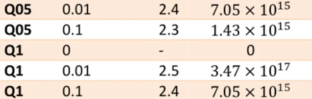
Bulk free ion concentration 𝒄𝟎 M 𝝍𝟎 V Charge density at surface 𝝆𝒄𝒉𝒂𝒓𝒈𝒆𝟎[𝑪𝒐𝒍𝒐𝒖𝒎𝒃𝒔𝒏𝒎𝟑 ] Q0 - - - Q05 0 - 0
14 Q05 0.01 2.4 7.05 × 10¹⁵ Q05 0.1 2.3 1.43 × 10¹⁵ Q1 0 - 0 Q1 0.01 2.5 3.47 × 10¹⁷ Q1 0.1 2.4 7.05 × 10¹⁵
Table 4: charge density at the surface for different surface potentials.
Once we know the charge density close to the surface we want to know how many ions are in that vicinity.
3.8 Number of counter ions at surface
To get a sense for how large the distance is between the ions one can imagine taking a
1 𝑛𝑚3 box at the surface where the charge
density is calculated as 𝜌0 in table 4. Since
the ions are monovalent, we can calculate the number of ions by taking the number of
ions in 1 𝑛𝑚3 as 𝑁 =𝜌0 𝑣 𝑒 = 7.05 [ 𝑐𝑜𝑢𝑙𝑜𝑚𝑏𝑠 𝑛𝑚3 ]× 1015× 1 [𝑛𝑚3] 1.6 × 10⁻¹⁹[𝑐𝑜𝑢𝑙𝑜𝑚𝑏𝑠 𝑖𝑜𝑛 ] 𝑁 = 4.4 × 1034 [𝑖𝑜𝑛𝑠]
For all the considered cases we thus get
Surface charge Bulk free ion concen-tration 𝒄𝟎 M Charge density at surface 𝝆𝒄𝒉𝒂𝒓𝒈𝒆𝟎[ 𝑪𝒐𝒍𝒐𝒖𝒎𝒃𝒔 𝒏𝒎𝟑 ] Number of particles N Q0 - - Q05 0 0 Q05 0.01 7.05 × 10¹⁵ 4.4 × 1034 Q05 0.1 1.43 × 10¹⁵ 8.9 × 1033 Q1 0 0 Q1 0.01 3.47 × 10¹⁷ 2.1 × 1036 Q1 0.1 7.05 × 10¹⁵ 4.4 × 1034 Table 4: charge density at the surface for different surface potentials and number of ions per 1 𝑛𝑚3
3.9 Inter ion separation
Now in the frame of Boltzmann statistics, assume that the ions are point charges. We want to know how much of the boxes volume if distributed equally is given to each ion.
Figure: Allocated volume to each ion. [3]
Imagine that each point charge gets a certain spherical volume. We then add the N spheres, and ask how large the radius of each sphere can be in order for N spheres
to make up the volume of a box of 1𝑛𝑚3.
4𝜋𝑟𝑠𝑝ℎ𝑒𝑟𝑒3
3 𝑁𝑖𝑜𝑛𝑠 = 𝑉𝑏𝑜𝑥 We then get that
𝑟𝑠𝑝ℎ𝑒𝑟𝑒 3 = 3𝑉𝑏𝑜𝑥 4𝜋𝑁𝑖𝑜𝑛𝑠
Taking the cube root we obtain
𝑟𝑠𝑝ℎ𝑒𝑟𝑒 = ( 3𝑉𝑏𝑜𝑥 4𝜋𝑁𝑖𝑜𝑛 ) 1 3
We take the volume of the box 𝑉𝑏𝑜𝑥to be
1 𝑛𝑚3 since we know the number of ions
per 𝑛𝑚3.To get an estimate of the distance
between the charges we then add two radii of adjacent spheres.
15 Thus the ion separation is
𝑟𝑠𝑒𝑝𝑒𝑟𝑎𝑡𝑖𝑜𝑛= 2 ( 3𝑉𝑏𝑜𝑥 4𝜋𝑁𝑖𝑜𝑛 ) 1 3
In the table below we list the acquired estimates. Surfac e charg e Bulk free ion conce n-tration 𝒄𝟎 M Charge density at surface 𝝆𝒄𝒉𝒂𝒓𝒈𝒆𝟎 [ 𝑪𝒐𝒍𝒐𝒖𝒎𝒃𝒔 𝒏𝒎𝟑 ] Numbe r of particl es N Inter-ion separatio n nm Q0 - - Q05 0 0 Q05 0.01 7.05 × 10¹⁵ 4.4 × 1034 3.6 × 10−36 Q05 0.1 1.43 × 10¹⁵ 8.9 × 1033 1.78× 10⁻³⁵ Q1 0 0 Q1 0.01 3.47 × 10¹⁷ 2.1× 1036 7.36 × 10−38 Q1 0.1 7.05 × 10¹⁵ 4.4 × 1034 3.6 × 10−36 Table 5
Thus the ionic separation is absurdly small and of course less than the minimum separation for the columbic interaction energy to be less than the thermal energy. We have therefore shown that.
𝑟𝐵 > 𝑟𝑖𝑜𝑛
Therefore the underlying assumptions for the Boltzmann statistics break down and thus solving the Poisson-Boltzmann
equation for this surface potential is vain.
3.10 Theoretical limit
In the given double layer thickness that is solely a function of the solvent and bulk concentration of ions, we are thus getting a charge density that is highly problematic since now the ions are so densely packed, that their charge and finite size becomes significant and causes the underlying assumptions for the Boltzmann statistics to break down. This implies that we need a second criteria for the Poisson-Boltzmann equation to give reasonable results. Looking at the expression for the charge density
sinh (𝜓(𝑥,𝑦,𝑧)𝑒 𝑞𝑖
𝑘𝐵𝑇 ) , we take the inverse of
the constants and get 𝑘𝐵𝑇
𝑒 = {𝑎𝑡 298𝐾} = 25.7 𝑚𝑉 We can use this quantity as a reference, to see how high the potential can be before the charge density gets out of control. We see that if
𝜓𝑞 ≤ 25.7 mV
Then there is not much charge density in
the double layer, since sinh (𝜓(𝑥,𝑦,𝑧)𝑒 𝑞𝑘 𝑖
𝐵𝑇 )
would not be very large. To be precise it would be less than or equal to 0.3818 [𝑪𝒐𝒍𝒐𝒖𝒎𝒃𝒔
𝒅𝒎𝟑 ]. If we however increase the
surface potential to 2.5 V so that the potential is 97.2 times larger than 25.7 mV,
then we would expect sinh (𝜓(𝑥,𝑦,𝑧)𝑒 𝑞𝑖
𝑘𝐵𝑇 ) and
consequently the charge density to be exponentially larger.
16
Figure: 𝜌𝑐ℎ𝑎𝑟𝑔𝑒= 𝑠𝑖𝑛ℎ (25.7𝑚𝑉 × 𝑛
26.7) for 𝑛 = 1,2, … ,10. Every time we increase the potential by 25.7 mV it means we are increasing the charge density by a factor of e. The red marked dots are were the theory is known to give reasonable results, that is 𝜓 < 80 𝑚𝑉.
We can generalize this procedure to find a relation that gives an upper limit for the surface potential.
As was stated above we require that
𝑟𝑠𝑒𝑝𝑒𝑟𝑎𝑡𝑖𝑜𝑛> 𝑟𝐵
This means that two times the radius of adjacent spheres need to be larger than the Bjerrum length 𝑟𝐵. 2 (3𝑉𝑏𝑜𝑥 4𝜋𝑁𝑖𝑜𝑛 ) 1 3 > 𝑟𝐵 We simplify (3𝑉𝑏𝑜𝑥 4𝜋𝑁𝑖𝑜𝑛 ) 1 3 >𝑟𝐵 2 Then cube both sides
(3𝑉𝑏𝑜𝑥 4𝜋𝑁𝑖𝑜𝑛
)>𝑟𝐵
3
8 Then solve for the number of ions
6𝑉
𝜋𝑟𝐵3 > 𝑁𝑖𝑜𝑛𝑠
If we now take a small volume at the
surface where the free ion charge density is
given by 𝜌0, we get that the number of ions
is
𝑁𝑖𝑜𝑛 =𝜌0𝑉
𝑒
Where 𝜌0 by Poisson-Boltzmann’s equation
is 𝜌𝑐ℎ𝑎𝑟𝑔𝑒0= 2𝑒𝑐0 𝜖0𝜖 𝑠𝑖𝑛ℎ (𝜓0𝑒 𝑘𝐵𝑇 ) So that 𝑁𝑖𝑜𝑛 = 𝑉 𝑒[ 2𝑒𝑐0 𝜖0𝜖 𝑠𝑖𝑛ℎ(𝜓0𝑒 𝑘𝐵𝑇 )] We obtain 6𝑉 𝜋𝑟𝐵3 > 𝑉 𝑒[ 2𝑒𝑐0 𝜖0𝜖 𝑠𝑖𝑛ℎ(𝜓0𝑒 𝑘𝐵𝑇 )] We then divide both sides by V and then isolate 𝑠𝑖𝑛ℎ(𝜓0𝑒 𝑘𝐵𝑇) 3𝜖0𝜖 𝜋𝑟𝐵3𝑐 0 > 𝑠𝑖𝑛ℎ(𝜓0𝑒 𝑘𝐵𝑇 )
We then take the inverse hyperbolic sine of both sides to get
sinh−1(3𝜖0𝜖
𝜋𝑟𝐵3𝑐0
) >𝜓0𝑒 𝑘𝐵𝑇
And then finally obtain the new relation we name the Wigner–Seitz-Boltzmann relation
𝑘𝐵𝑇 𝑒 sinh
−1(3𝜖0𝜖
𝜋𝑟𝐵3𝑐0 ) > 𝜓0
For a solvent with a dielectric constant of 78. At 298K with a monovalent salt at 𝑐 = 0.1𝑀 the Wigner–Seitz-Boltzmann relation thus gives the theoretical maximum
potential to be
17 For a monovalent free ion concentration of 𝑐 = 0.01𝑀
519 𝑚𝑉 > 𝜓0
These upper limits should however be taken with a grain of salt as it is generally
accepted that the Poisson-Boltzmann equation gives reasonable results for surface potentials up to 80mV [7], this corresponds to a free ion charge density at
the surface of 3.7903 [𝑪𝒐𝒍𝒐𝒖𝒎𝒃𝒔𝒅𝒎𝟑 ]. The
Wigner–Seitz-Boltzmann relation gives the maximum surface potential only in the sense that the electrostatic interaction between the ions don’t violate the Boltzmann statistics.
3.11 Conclusion
In this study we have confirmed that the interaction potential energy between cellulose nanofibrils surface substituted with TEMPO oxidation cannot be modeled
with the Poisson-Boltzmann equation, as the surface potential is too high for
Boltzmann statics to hold. This parts of the study is therefore inconclusive. We can however conclude that for highly charged fibrils modeled with no free ions, where we don’t rely on Boltzmann statistics and thus the Poisson equation is valid, the dipole interactions appear to be negligible in comparison to the surface charge
contribution to the interaction potential. Furthermore we have combined the Bjerrum length, The Poisson-Boltzmann equation and the Wigner–Seitz radius to derive a new relation called the Wigner– Seitz-Boltzmann relation that predicts the theoretical upper limit for the surface potential for the Poisson-Boltzmann equation applied to monovalent free ionic solutions strictly in terms of bulk
18
19 In the appendices below, we first discuss
the concepts of charge interactions in free space, in particular the relationship
between force and potential energy, and then derive the equations that extend charge interactions in solutions, with and without the presence of free ions.
Appendix A – Electrostatic force
Point charges are defined as charges for
which the particle diameter is much smaller than the interparticle distance Assume two point charges residing in space at the points (𝑥1, 𝑦1, 𝑧1) and (𝑥2, 𝑦2, 𝑧2). The position of
those charges in 𝑅³ can be described by the vector:
𝑟⃗𝑖(𝑥, 𝑦, 𝑧) =< 𝑥𝑖, 𝑦𝑖, 𝑧𝑖 >
This is a vector pointing from the origin to the to the point charge, see the figure below. The force acting between those two point charges in vacuum depends on the radial distance between them and the magnitude and signs of their charges respectively, it is stated by Coulomb’s Law as: 𝐹⃗ = 1 4𝜋𝜖0 𝑞1𝑞2 |𝑟⃗2− 𝑟⃗1| (𝑟⃗2− 𝑟⃗1)
As is seen by Coulomb's law the force vector between two point charges will
always point in the direction 𝑟⃗2− 𝑟⃗1, which
is always parallel or antiparallel to the line AB connecting them in space. Depending on the sign of the charges, the force will either act attractively on both charges
simultaneously with equal magnitude or repel them both with equal magnitude.
Force field from distribution of point charges
Instead of looking at the interaction between two charges, let’s look at the interaction between a distribution of
charges on some hypothetical charge that is placed anywhere in space with position vector 𝑟⃗(𝑥, 𝑦, 𝑧). The force acting between each charge and the hypothetical is again given by coulomb's law. Being a vector quantity the vector sum will give the
direction and magnitude of the net force on that particle. 𝛴𝐹⃗ = 1 4𝜋𝜖0 𝑞1𝑞2 |𝑟⃗2− 𝑟⃗1| (𝑟⃗1− 𝑟⃗0)+. . . + 1 4𝜋𝜖0 𝑞𝑛𝑞0 |𝑟⃗𝑛− 𝑟⃗0| (𝑟⃗𝑛− 𝑟⃗0) 𝛴𝐹⃗(𝑟⃗⃗⃗⃗⃗⃗ =0) 𝑞0 4𝜋𝜖0 ∑ 𝑞𝑖 |𝑟⃗𝑖− 𝑟⃗0| (𝑟⃗𝑖− 𝑟⃗0) 𝑛 𝑖=1
The ability to add force vectors is known as the superposition principle. If the force is calculated at every point for some
hypothetical point q, then we obtain the force field from that distribution of charges. If we divide the force field equation by the hypothetical charge, we obtain the
equation. 𝐸⃗⃗ = 1 4𝜋𝜖( 𝑞1 𝑟1²𝑟⃗1+. . . + 𝑞𝑛 𝑟𝑛²𝑟⃗𝑛)= 1 4𝜋𝜖∑ 𝑞𝑖 𝑟𝑖²𝑟⃗⃗⃗𝑖 𝑛 𝑖
This is known as the electric field and describes how a distribution of point charges affect other charges in the space around them by defining a vector at every point (x,y,z). This vector can be seen as the force per unit charge due to that
distribution of point charges at a given point. The advantage of the electric field concept over the force field concept is that we can visualize how positive and negative charges alter space separately. Notice that the electric field emanating from a single
20 positive charge always is diverging
outwards in all directions like a source and for negative charges the electric field will converge like a sink. [8].
Figure 1: Electric field line from positive and negative charges.
Appendix B – Divergence
To make the concept of divergence clear lets make an analogy. Suppose we are standing in a river and as ridiculous as it sounds we are only interested in a two dimensional part of the river, so you may imagine we are standing in a slice of this river, so that we can only move in the x and y direction. Suppose at some location in this river we wish to measure the force that the river exerts in all directions from that point. How would one measure this? One way would be to walk around this point, and hold out some kind of spring connected to a board that reacts to the pressure force of the water. Lets call the oriented path that we walk around this point 𝑑𝛺 and let it for simplicity be the boundary of a square. Now all we need to do is to sum up all the
measurements that we made along this path and we will get a scalar value that estimates how much force is coming from that point that was normal to the board along the whole path. Now depending on how many points we made the
measurement on and how small the area of the boundary enclosed by the path 𝑑𝛺 was, we will get different accuracy of this
measurement of the force in all directions or more formally the divergence of that
force field at that point.
Now lets write this concept mathematically.
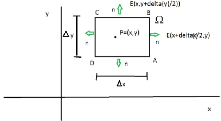
figure: Square boundary 𝛺 around point P.
Suppose 𝐸⃗⃗(𝑥 , 𝑦) is a vector field in 𝑅2 .
Now suppose we draw a square boundary around a point P and call the boundary 𝛺. Then the magnitude of the field normal to the boundary at every point along the boundary curve is given by the dot product of the field 𝐸⃗⃗(𝑥 , 𝑦) with the normal vector 𝑛⃗⃗(𝑥, 𝑦) to the boundary curve. The dot product 𝐸⃗⃗(𝑥, 𝑦) ∙ 𝑛⃗⃗(𝑥, 𝑦) can be seen as the magnitude of the field 𝐸⃗⃗(𝑥, 𝑦) in the direction of 𝑛⃗⃗(𝑥, 𝑦).
Figure 2. Dot product: the dot product of the vector A and B is the length (magnitude) of A in the direction of B.
The smaller we let the boundary 𝑑Ω get and the more points we measure in the outward
21 directed field along the boundary curve, the more accurate measure of the divergence one obtains. So one needs to take the limit of the sum of the dot products as the area of the boundary goes to zero. Take our limit variable h to be ℎ = 2𝛥𝑥 + 2𝛥𝑦, so that when h goes to zero both 𝛥𝑥 → 0 and 𝛥𝑦 → 0 , and thus Δ𝑥Δ𝑦 must go to zero. Note that h can be thought of the circumference of the boundary.
Then we can write the divergence as 𝑑𝑖𝑣𝑒𝑟𝑔𝑒𝑛𝑐𝑒 𝑜𝑓 𝐸⃗⃗(𝑥, 𝑦) = 𝑙𝑖𝑚 𝛥𝑥,𝛥𝑦→0 1 𝛥𝑥𝛥𝑦∮ 𝐸⃗⃗(𝑥, 𝑦)𝑑Ω ∙ 𝑛⃗⃗ 𝑑𝑥𝑑𝑦
Since line integrals are additive operators, we may break the closed loop integral into four segments. We evaluate the integral at all sides of the boundary going counter clockwise from A to D. Along the sides, the electric field is given by:
AB 𝐸⃗⃗(𝑥 +𝛥𝑥2 , 𝑦), CD 𝐸⃗⃗(𝑥 −𝛥𝑥 2 , 𝑦) BC 𝐸⃗⃗(𝑥, 𝑦 +𝛥𝑦 2) DA 𝐸⃗⃗(𝑥, 𝑦 −𝛥𝑦 2)
Furthermore since the normal on this square boundary is always directed either towards the positive and negative y and x axis, we will always take the normal vector pointing out of the boundary, we may replace 𝑛⃗⃗ with ±𝑥⃗ and ±𝑦⃗, which are unit vectors.
Therefore the closed loop integral is written as the sum 𝑙𝑖𝑚 𝛥𝑥,𝛥𝑦→0 1 𝛥𝑥𝛥𝑦∮ 𝐸⃗⃗(𝑥, 𝑦) ∙ 𝑛⃗⃗ 𝑑𝛺𝛺 = 𝑙𝑖𝑚 𝛥𝑥,𝛥𝑦→0 1 𝛥𝑥𝛥𝑦(∫𝐴𝐵+𝐶𝐷𝐸⃗⃗(𝑥, 𝑦) ∙ 𝑥⃗ 𝑑𝑦 + ∫𝐵𝐶+𝐷𝐴𝐸⃗⃗(𝑥, 𝑦)∙ 𝑦⃗𝑑𝑥)
Whereas seen from the figure:
∫ 𝐸⃗⃗(𝑥, 𝑦) ∙ 𝑛⃗⃗⃗⃗⃗ 𝑑𝑦 𝐴𝐵+𝐶𝐷 = (∫ 𝐸⃗⃗ (𝑥 +𝛥𝑥 2 , 𝑦) ∙ 𝑥⃗ 𝑑𝑦 Δy − ∫ 𝐸⃗⃗ (𝑥 −𝛥𝑥 2 , 𝑦) ∙ 𝑥⃗ 𝑑𝑦 Δy )
The reason we can integrate on Δy is that the change of sign of the normal vector
takes into account the orientation
And ∫ 𝐸 ⃗⃗⃗⃗(𝑥, 𝑦) ∙ 𝑛⃗⃗ 𝑑𝑥 𝐵𝐶+𝐷𝐴 = ∫ 𝐸⃗⃗ (𝑥, 𝑦 +𝛥𝑦 2) ∙ 𝑦⃗ 𝑑𝑥 Δx − ∫ 𝐸⃗⃗(𝑥, 𝑦 −𝛥𝑦 2) ∙ 𝑦⃗ 𝑑𝑥 Δ𝑥
The dot product of 𝐸⃗⃗ (𝑥 ±Δ𝑥2 , 𝑦) ∙ ±𝑥⃗⃗⃗⃗⃗⃗ is
independent of y, as the unit vector 𝑥⃗ = 〈1,0〉.
𝐸⃗⃗ (𝑥 ±Δ𝑥
2 , 𝑦) ∙ ±〈1,0〉 = ±E (𝑥 ± Δ𝑥
2) We can thus bring out the expression from under the integral sign and we acquire the expression: 𝑙𝑖𝑚 𝛥𝑥,𝛥𝑦→0 1 𝛥𝑥𝛥𝑦(𝛥𝑦𝐸⃗⃗⃗⃗ (𝑥 + 𝛥𝑥 2)∙ 𝑥⃗⃗⃗− 𝛥𝑦𝐸⃗⃗⃗⃗ (𝑥 − 𝛥𝑥 2)∙ 𝑥⃗⃗⃗) Which simplifies to 𝑙𝑖𝑚 𝛥𝑥→0 𝐸⃗⃗(𝑥 +𝛥𝑥2) ∙ 𝑥⃗ − 𝐸⃗⃗(𝑥 −𝛥𝑥2) ∙ 𝑥⃗ ) 𝛥𝑥
Which we know as the directional
derivative of E(x,y) as a function of x parallel to the x-axis 𝑙𝑖𝑚 𝛥𝑥→0 𝐸⃗⃗(𝑥 +𝛥𝑥2) ∙ 𝑥⃗ − 𝐸⃗⃗(𝑥 −𝛥𝑥2) ∙ 𝑥⃗ 𝛥𝑥 = 𝑑𝐸⃗⃗(𝑥, 𝑦) 𝑑𝑥 𝑥⃗
22 By the same argument for the other sides of the boundary we obtain
𝑙𝑖𝑚 𝛥𝑦→0 𝐸⃗⃗(𝑦 +𝛥𝑦2) ∙ 𝑦 − 𝐸⃗⃗(𝑦 −𝛥𝑦2) ∙ 𝑦 ) 𝛥𝑦 = 𝑑𝐸⃗⃗(𝑥, 𝑦) 𝑑𝑦 𝑦⃗
Note that these values are both scalars since it is the dot product of two vectors. We thus conclude that
𝑑𝑖𝑣𝑒𝑟𝑔𝑒𝑛𝑐𝑒 𝑜𝑓 𝐸⃗⃗(𝑥, 𝑦) =𝑑𝐸⃗⃗(𝑥, 𝑦) 𝑑𝑥 𝑥⃗ + 𝑑𝐸⃗⃗(𝑥, 𝑦) 𝑑𝑦 𝑦⃗ or more compactly 𝛻𝐸⃗⃗ =𝑑𝐸⃗⃗(𝑥, 𝑦) 𝑑𝑥 𝑥⃗ + 𝑑𝐸⃗⃗(𝑥, 𝑦) 𝑑𝑦 𝑦⃗
Where 𝛻𝐸⃗⃗ is known as the divergence of the field𝐸⃗⃗. Divergence can in other words be estimated at any point as the scalar sum of the directional derivatives of the vector function, parallel to the vectors that span the space. [9]
Appendix C – Gauss's theorem and
law of electrostatics
Suppose a charge is enclosed in an imaginary surface S as in figure 4.
Figure4: Charged enclose by imaginary sphere [8]
Then the net charge within that closed surface is related to the net flux of the electric field throughout the whole surface
by Gauss’s law
𝜙 = ∫ ∫ 𝐸⃗⃗ 𝒅𝑨⃗⃗⃗
𝑆
=𝑄𝑒𝑛𝑐𝑙𝑜𝑠𝑒𝑑 𝜖
Gauss’s law is valid for any closed surface, and in essence states the same thing as Coulomb's law and the superposition principle combined [8]. This means that it is a statement of electrostatics and is valid when there is no acceleration or when the
charges are moving very slowly. A more useful way of expressing the flux through the surface in terms of the enclosed charge, is in terms of the divergence of the electric field. By the divergence theorem the total flux through the surface S is equal to the divergence of the vector field E within the whole volume V enclosed by S.
∫ ∫ 𝐸 ∙⃗⃗⃗⃗⃗ 𝒅𝑨⃗⃗⃗
𝑆
= ∫ ∫ ∫ 𝛻𝐸⃗⃗ 𝑑𝑉
𝑉
Where 𝛻𝐸⃗⃗ is as stated above the divergence of the field𝐸⃗⃗.
To understand this theorem lets go back to the definition of divergence. Since we worked on a two dimensional space we will continue this argument here, however this can be extended to real space as well. Suppose we take a region, bounded by the blue box. Then we calculated the
23 sum of the dot product of the electric field with the normal vector to the boundary 𝑑𝛺. Now suppose that within the area of the blue box, we wish to sum all the divergence. That basically means
𝑇𝑜𝑡𝑎𝑙 𝑑𝑖𝑣𝑒𝑟𝑔𝑒𝑛𝑐𝑒 = ∫ ∫ 𝑑𝑖𝑣(𝐸) 𝑑𝑥𝑑𝑦
𝛥𝑥 𝛥𝑦
Now note that, as we move counter clockwise around every square 𝛺 and sum up the electric field component in the normal direction, there is always another square next to it that goes in the exact opposite direction at that point. This means that when we sum up all the divergence within the box, all the interior divergences will cancel and only the components at the boundary will contribute to the total
divergence. This means we may say that the total divergence within the region is equal to the line integral around the boundary for that field. 𝑇𝑜𝑡𝑎𝑙 𝑑𝑖𝑣𝑒𝑟𝑔𝑒𝑛𝑐𝑒 = ∫ 𝛥𝑦 ∫ 𝑑𝑖𝑣(𝐸) 𝑑𝑥𝑑𝑦 𝛥𝑥 = ∮ 𝐸⃗⃗ 𝑑𝐶 𝐶
This is Gauss's theorem in 𝑅2.
With the same line of reasoning where the points are in space, and we calculate the divergence as the volume around the point goes to zero, and we sum all the divergence within a body, we get the same result, only now we are integrating over a volume and all small divergences within this volume cancel, so that we can equate the total divergence as the sum of the dot product between the electric field and the area vector of the surface. [9]
Now rewriting the right hand side of
Gauss’s law, the charge enclosed is the same thing as the volume integral of the
charge density 𝜌𝑐ℎ𝑎𝑟𝑔𝑒 on all of V.
𝑄𝑒𝑛𝑐𝑙𝑜𝑠𝑒𝑑 = ∫ ∫ ∫
𝜌𝑐ℎ𝑎𝑟𝑔𝑒
𝜖 𝑑𝑉
𝑉
It follows that Gauss’s law may be rewritten as
𝜙 = ∫ ∫ 𝐸⃗⃗ 𝒅𝑨⃗⃗⃗ 𝑆 =𝑸𝒆𝒏𝒄𝒍𝒐𝒔𝒆𝒅 𝝐 = ∫ ∫ ∫ 𝜌𝑐ℎ𝑎𝑟𝑔𝑒 𝜖 𝑑𝑉 𝑉 and therefore ∫ ∫ ∫ 𝛻𝐸⃗⃗ 𝑑𝑉 𝑉 = ∫ ∫ ∫ 𝜌𝑐ℎ𝑎𝑟𝑔𝑒 𝜖 𝑑𝑉 𝑉 so that 𝛻𝐸⃗⃗(𝑥, 𝑦, 𝑧) =𝜌𝑐ℎ𝑎𝑟𝑔𝑒(𝑥,𝑦,𝑧) 𝜖
We conclude therefore that the divergence of the electric field at any point within the volume V is equal to the total flux through the closed surface S and is therefore equal to the charge density within that volume at every point. [10]
Appendix D – Potential energy
When a charge moves in a force fields, along a directed path C, see figure 6, the work done by the field during the
displacement is given by the vector line integral
𝑊 = − ∫ 𝐹⃗ ∙ 𝑑𝑙⃗⃗⃗⃗
𝐶
This line integral may be interpreted as the sum of the dot products of the force field vector 𝐹⃗ with the tangential component of the displacement vector along the curve C, or equivalently the sum of the infinitesimal
24 work elements along this trajectory. [11]
Viewing the colloid as a charged particle, or collection of charged particles moving as one unit and neglecting the work to
displace ions and gravity, the energy used is given purely as the work need to displace the colloid against the Columbic force of the other fibrils and the ions in the
environment.
figure 6: Trajectory along curved path C [11]
This way of viewing particle interactions is known as charge dynamics, chemists however are more interested in interaction energies. We will therefore derive a set of equations that relate the interaction energies between charged particles with the forces acting between them, and then purely reason in terms of energy. This is however only possible for certain kinds of force fields which we will explore now.
Relating force and energy
One class of vector fields possess the property that when integrated upon from a point A to B, the value of the integral is independent of the path taken. Such a field is called conservative. [8] When a force field is conservative, the work done by that field may be expressed in terms of the values of the potential energies U at the starting and end points. Potential energy is defined as the amount of work needed in order to bring a charged particle to its present position in a force field from an
infinite distance where the potential is arbitrarily set as zero. The work in a
conservative field is given by the expression 𝑊 = − ∫ 𝐹⃗ ∙ 𝑑𝑙⃗⃗⃗⃗
𝐶
= 𝑈(𝐴) − 𝑈(𝐵) where
𝑈 𝑖𝑠 𝑡ℎ𝑒 𝑠𝑐𝑎𝑙𝑎𝑟 𝑝𝑜𝑡𝑒𝑛𝑡𝑖𝑎𝑙 𝑒𝑛𝑒𝑟𝑔𝑦 𝑎𝑡 𝑎 𝑔𝑖𝑣𝑒𝑛 𝑝𝑜𝑖𝑛𝑡 The electrostatic work on charged particles in electric fields is slightly different than the gravitational work on bodies in gravitational fields as gravity only acts attractively on bodies, however since charged particles can be both positive and negative, electric fields can both repel and attract. It is customary to work with positive charges as a standard and we define work to be positive when work is done in the direction of the field. Furthermore for this relation to hold, the following equation must also be true by the fundamental theorem of vector fields.
𝑊 = ∫ 𝛻𝑈 ∙ 𝑑𝑙𝐶 ⃗⃗⃗⃗= 𝑈(𝐴) − 𝑈(𝐵) where 𝛻𝑈 =<𝑑𝑈 𝑑𝑥, 𝑑𝑈 𝑑𝑦, 𝑑𝑈 𝑑𝑧 >
Is the gradient of the scalar function U(x,y,z). The gradient of a scalar function is a vector field whose components are the partial derivatives of the function and is always directed in the direction of maximum change of that function.
It follows that 𝑊 = ∫ 𝐹⃗ ∙ 𝑑𝑙⃗⃗⃗⃗ 𝐶 = − ∫ 𝛻𝑈 ∙ 𝑑𝑙⃗⃗⃗⃗ 𝐶 and thus
25 𝐹⃗ = −𝛻𝑈
This equation states that the force field always is directed towards lower potential energy. So essentially the force field will always move a particle to the position of lowest potential energy. This result bridges charge dynamics and energetics.
Appendix E – Columbus law
It now remains to be seen if the force field between charged particles is a conservative field. We will verify this by the following argument. In a conservative force field, as stated above, the work done when going between two points is the difference in the potential energy U. Therefore, if the force field described by Coulomb's law abides to this definition then we can be certain that the force field between charged particles is conservative. While showing this we will illustrate an important consequence of conservative fields, namely conservation of energy.
Suppose a positively charged particle established a force field, as seen in figure 3. Then the work done when moving a charge from point A to B is given by:
figure 7 [8] 𝑊 = ∫ 𝐹⃗ ∙ 𝑑𝑙𝐶 ⃗⃗⃗⃗= ∫ |𝐹⃗|𝑐𝑜𝑠(𝜃)𝑑𝑙𝑟𝑏 𝑟𝑎 = {𝑑𝑟 = 𝑐𝑜𝑠(𝜃)𝑑𝑙} = ∫ 4𝜋𝜖1 𝑞0𝑞 𝑟² 𝑑𝑟 𝑟𝑏 𝑟𝑎
Integrating with respect to the radial component 𝑊 =𝑞0𝑞 4𝜋𝜖∫ 1 𝑟2𝑑𝑟 𝑟𝑏 𝑟𝑎 = 𝑞0𝑞 4𝜋𝜖( 1 𝑟𝑎 − 1 𝑟𝑏 ) = 𝑞0𝑞 4𝜋𝜖𝑟𝑎 − 𝑞0𝑞 4𝜋𝜖𝑟𝑏 = 𝑈(𝑟𝐴) − 𝑈(𝑟𝑏)
We obtain the relation we would expect from a conservative field, namely
𝑊 = −𝛥𝑈
As is seen above the work done when moving a charge in the field described by Coulomb's law is just the difference in potential energy, and explicitly the potential energy at any point is given by
𝑈(𝑟) = 𝑞0𝑞 4𝜋𝜖𝑟
A consequence of this is that the work done when moving from a point A to any point B, and then back to A, or going in a closed loop, the work is given by the closed loop integral
𝑊 = ∮ 𝐹⃗𝑑𝑙
𝐶
= 𝑈(𝑟𝑎) − 𝑈(𝑟𝑎) = 0
This means that all electric work is
reversible and thus energy in this system is always conserved, by the law of
conservation of energy it then alternates between kinetic energy K and potential energy U.
𝑈𝐴+ 𝐾𝐴 = 𝑈𝐵+ 𝐾𝐵
It is important to note that if the field is not conservative, the energy changes cannot be
26 expressed as potential energies U but
rather changes in internal energies. [8][11]
Appendix F – The Poisson equation
We will go even further than this and derive the relationship between the electric field interactions of charged particles and the potential energy on a per charge basis.
𝐹⃗ = 𝐸⃗⃗𝑞 = −𝛻𝑈 𝐸⃗⃗ = −𝛻𝑈
𝑞 = −𝛻𝜓
Where 𝜓is known as the potential and is given in the units of volts.
Note that if the force field is conservative then this must also mean that the electric field is a conservative field. We can now find the potential anywhere in space by combining gauss’s law with the relations between the electric field and the potential gradient.
Since the electric field is conservative we concluded that
𝐸⃗⃗ = −𝛻𝜓
By Gauss’s law the divergence of the
electric field was proportional to the charge density 𝛻𝐸⃗⃗ =𝜌𝑐ℎ𝑎𝑟𝑔𝑒 𝜖 Therefore 𝛻𝐸⃗⃗ = −𝛻²𝜓 =𝜌𝑐ℎ𝑎𝑟𝑔𝑒 𝜖 This relation is known as Poisson's equation. Where ∇2𝜓 =𝑑²𝜓 𝑑𝑥²+ 𝑑²𝜓 𝑑𝑦²+ 𝑑²𝜓 𝑑𝑧² So that 𝑑²𝜓 𝑑𝑥²+ 𝑑²𝜓 𝑑𝑦² + 𝑑²𝜓 𝑑𝑧² = − 𝜌𝑐ℎ𝑎𝑟𝑔𝑒 𝜖 It is an elliptic second order partial
differential equation, whose solution is the scalar function 𝜓(𝑥, 𝑦, 𝑧), which maps the potential distribution in space given the
charge distribution 𝜌𝑐ℎ𝑎𝑟𝑔𝑒. [7] [10]
Appendix F-2 – The Laplacian of 𝝍
𝛻²𝜓 is called the Laplacian of the potential and relates the potential 𝜓(𝑥, 𝑦, 𝑧) to the
average potential 𝜓𝑎𝑣𝑒𝑟𝑎𝑔𝑒 around the
point (𝑥, 𝑦, 𝑧). If
𝛻2𝜓 > 0
Then from Poisson’s equation 𝜌𝐶ℎ𝑎𝑟𝑔𝑒 < 0
meaning that the local charge density is negative, or equivalently that at (𝑥, 𝑦, 𝑧) there is a net excess of negative ions. Then
𝜓 < 𝜓𝑎𝑣𝑒𝑟𝑎𝑔𝑒
Meaning that the potential at that point is lower than the average potential in that vicinity. The converse can be said when the
∇2𝜓 < 0 and 𝜌
𝑐ℎ𝑎𝑟𝑔𝑒 > 0.
When
∇2𝜓 = 0
The charge density is zero and the negative and positive ion charges perfectly cancel, then
27 The potential at that point is equal to the
average potential in that vicinity. [11] [12]
Appendix F-3 – Solution to Poisson’s equation
What would we expect the potential drop to be like if we have no free ions? That is
when 𝜌𝑐ℎ𝑎𝑟𝑔𝑒 = 0
∇2𝜓 = 0
Let’s for simplicity assume that 𝜓 only varies with x, so that we may say instead
𝑑2𝜓
𝑑𝑥2 = 0
To solve for 𝜓 we integrate with respect to x, where x is the distance from the charged surface.
𝑑𝜓 𝑑𝑥 = 𝐴
Where A is some integration constant, which we will determine with the boundary conditions. Integrating again to obtain 𝜓 we get
𝜓(𝑥) = 𝐴𝑥 + 𝐵 Now we impose the constraints that
𝜓(0) = 𝜓0
𝜓(𝑘) = 0
Meaning that the potential at the surface is the surface potential and that the potential drops to zero at some finite distance 𝑥 = 𝑘. Thus we see that when there are no free ions in the solution, Poisson’s equation predicts that the potential will drop linearly with distance from a charged surface.
28