Investigating Performance of Different Models at Short Text Topic Modelling

STOCKHOLM, SWEDEN 2020

Investigating

Performance of

Different Models at

Short Text Topic

Modelling

KTH Thesis Report

Pratima Rao Akinepally

En jämförelse av textrepresentationsmodellers prestanda tillämpade för ämnesinnehåll i korta texter

Authors

Pratima Rao Akinepally <prak@kth.com> Computer Science and Engineering

KTH Royal Institute of Technology

Project conducted at

Stockholm, Sweden Spotify AB

Examiner

Pawel Herman

KTH Royal Institute of Technology

Supervisor

Jussi Karlgren

KTH Royal Institute of Technology

Supervisor at

Spotify AB

The key objective of this project was to quantitatively and qualitatively assess the performance of a sentence embedding model, Universal Sentence Encoder (USE), and a word embedding model, word2vec, at the task of topic modelling. The first step in the process was data collection. The data used for the project was podcast descriptions available at Spotify, and the topics associated with them. Following this, the data was used to generate description vectors and topic vectors using the embedding models, which were then used to assign topics to descriptions. The results from this study led to the conclusion that embedding models are well suited to this task, and that overall the USE outperforms the word2vec models.

Keywords

Det huvudsakliga syftet med det i denna uppsats rapporterade projektet är att kvantitativt och kvalitativt utvärdera och jämföra hur väl Universal Sentence Encoder USE, ett semantiskt vektorrum för meningar, och word2vec, ett semantiskt vektorrum för ord, fungerar för att modellera ämnesinnehåll i text. Projektet har som träningsdata använt skriftliga sammanfattningar och ämnesetiketter för podd-episoder som gjorts tillgängliga av Spotify. De skriftliga sammanfattningarna har använts för att generera både vektorer för de enskilda podd-episoderna och för de ämnen de behandlar. De båda ansatsernas vektorer har sedan utvärderats genom att de använts för att tilldela ämnen till beskrivningar ur en testmängd. Resultaten har sedan jämförts och leder både till den allmänna slutsatsen att semantiska vektorrum är väl lämpade för den här sortens uppgifter, och att USE totalt sett överträffar word2vec-modellerna.

Nyckelord

Textanalys, semantiska vektorrum, NLP, word2vec, Universal Sentence Encoder, Poddar

There are several people I would like to thank for helping and guiding me through the course of this project. First and foremost, I would like to thank Prof. Jussi Karlgren, my supervisor from KTH, for providing me with useful inputs and advice during my project. I would also like to thank my supervisor from Spotify, Maria Movin, for overseeing the work and providing the necessary technical support. I am also thankful to the rest of the Search Team at Spotify for their valuable feedback.

Finally, I would be remiss if I did not take the opportunity to thank my friends for their encouragement and for proofreading my report.

NLP Natural Language Processing

NLU Natural Language Understanding

GPT Generative Pre-Training

BERT Bidirectional Encoder Representations from Transformers

USE Universal Sentence Encoder

WEF World Economic Forum

SVM Support Vector Machine

LSTM Long short-term memory

CNN Convolutional neural network

BOW Bag-of-Words

tf idf term frequency-inverse document frequency

CBOW Common Bag-of-Words

LSA Latent Semantic Analysis

LDA Latent Dirichlet Allocation

IR Information Retrieval

RAKE Rapid Automatic Keyword Extraction

1 Introduction

1

2 Theoretical Background

5

2.2 Short Text Classification . . . 7

2.3 Representing Text . . . 7 2.4 Word Embeddings . . . 8 2.5 Sentence Embeddings . . . 11 2.6 Topic Modelling . . . 14 2.7 Topic Assignment . . . 15

3 Method

19

3.1.3 Test Set 1: Descriptions assigned with the correct label . . . 21

3.1.4 Test Set 2: Descriptions with labels from existing model . . . 21

3.1.5 Training and Testing Data . . . 21

3.2 Implementation . . . 22

3.2.1 Model Architectures . . . 22

3.2.2 Generating description vectors and topic vectors . . . 23

3.2.3 Assigning Labels . . . 24

4 Results

27

4.1 Accuracy with Keyword Extraction . . . 27

4.2 Overall Accuracy . . . 28

4.3 Comparing with existing model . . . 29

4.4 Error Analysis and Discussion . . . 31

4.4.1 USE error analysis. . . 31

4.4.2 Difference in performance across models . . . 37

5 Discussion

39

5.2 Benefits, Ethics and Sustainability . . . 41

6 Conclusions

42

Introduction

Podcasts are audio files that contain spoken word content. They can be monologues, interviews or discussions, covering a wide range of topics. This form of media has been growing increasingly popular, with an estimated 155 million people listening to podcasts every week in 20201_{. This rapid growth in popularity has also meant an}

increase in the podcast content being created. To keep up with the new media, and to better serve users seeking this content, it is essential to find better ways of handling and sorting through this data. One way of doing this is by annotating the podcasts with ‘topics’ or labels that capture the relevant information about the podcast.

In this context, a topic is a general term which captures the subject covered in a text. More intuitively, these are words that give us an idea of what a text is about, but it is hard to capture exactly what categorises a word as a topic. This is because these topics are dependent on a variety of factors such as the context, the readers’ point of view and preference, the task for which it is being used etc. Additionally, the words themselves can be ambiguous and convey different meanings in different contexts. The term carrot in a text might be used in the context of agriculture, cooking, meals, cultural history, education or economy (stick and carrot). And in each of these contexts, the ’carrot’ has a different degree of importance when it comes to assigning labels.

Spotify, a media services provider, uses podcast descriptions (in text form) to generate and assign topics to podcasts. These descriptions are provided by the content creators at the time of publishing content on the platform. The topics are generated by applying

keyword extraction on the descriptions. However, there are two key limitations with this approach. The first one being that in some instances the algorithm picks up redundant words like podcast, episode, URLs etc. as keywords, and second one being that the word has to be explicitly mentioned in the description for it to be a potential topic. For example, a podcast discussing football which does not have the word sport in the description, can never be assigned sport as a topic. Such a system cannot understand the semantic content of the text and provide context dependent topics.

The goal of the thesis project was to move beyond a simple keyword extraction technique, and use Topic Modelling to improve the quality of topics annotated to podcast descriptions. Topic Modelling is an unsupervised machine learning technique which allows for the inference and understanding of the ’topics’ associated with a text [22]. Additionally, it also captures the relevance of a text with regard to a particular topic. Topic models start from the assumption that texts have multiple topics, and that each observable linguistic item (i.e. a word) provides evidence for a topic [5], and frequently provides evidence for many topics. These models assist with the task of handling large amounts of unlabelled data, by assigning texts with certain topics and keywords based on the content. This is especially useful in the fields of Search Optimization, wherein understanding the text can allow the search engine to retrieve relevant results [36]. The approach of the project involves finding an embedding for the podcast descriptions and using this to assign topics to the podcasts.

1.1

Problem

Topic models cover a wide variety of models from those based on a simple Bag-of-Words approach, to probabilistic models or even more complex Machine Learning models. The current trend in the field of topic modelling is to use pre-trained word embeddings, which are numerical vector representations of words, trained on transfer tasks. This trend began in 2018 with the introduction of Generative Pre-Training (GPT) [42] and Bidirectional Encoder Representations from Transformers (BERT) [11], and was developed further by models like ALBERT[27], RoBERTa [32], GPT-2. All of the models, however, are word embeddings.

paragraphs into a vector space. The techniques involved in producing sentence embeddings range from simply averaging word embeddings, to unsupervised and supervised approaches, including newer multi-task learning approaches. Sentence embeddings have been shown to outperform word level transfer [6]. Introduced in 2018, Google’s USE [6] is a state of the art model for the task of sentence embedding. The method using of a pre-trained embeddings has brought with it a wave of state of the art results in the field.

The overarching goal of this thesis project is to qualitatively and quantitative assess the performance of different embedding models at the task of topic modelling, and to evaluate whether or not sentence embeddings are a worthwhile option for this task. The project also seeks to find the difference in performance between sentence and word embedding models.

1.1.1

Research Question

How does a pre-trained, state-of-the-art sentence embedding model - USE [6] compare to simpler, task specific word2vec that are built using only relevant data?

The main problem has been broken down into the following objectives:

1. To compare the performance of task specific word embeddings with a general pre-trained word embedding model in terms of accuracy of predicted labels. 2. To compare and rank the performance of the USE, pre-trained word2vec and

in-house word2vec using accuracy of predicted labels as the metric of choice. 3. To compare the performance of the sentence embedding model, USE to word

embedding models in terms of manual evaluation of relevance of predicted labels. 4. To assess whether it is necessary to build simpler, task specific models when a

pre-trained sentence encoder can be used.

By addressing these, the thesis also aims to find out whether it is worthwhile to train an in-house, task specific USE. If the performance of a simpler, task specific model is comparable to that of the pre-trained Sentence Encoder, it would be fair to assume a Sentence Encoder trained specifically on the task of label prediction for podcast descriptions would show very good performance.

1.2

Outline

The report is comprised of five chapters. The first one, Introduction, provides an overview of the project and states the key research questions the thesis aims to answer. This is followed by a chapter on the Theoretical Background. In Chapter 3, Method, all the components used in the project such as data, the model architectures and methodology, and the evaluation metrics are described. Chapter 4, Results, explains all the experiments conducted during the project and the corresponding results. This chapter also includes a section on Error Analysis. Chapter 5, Discussion, summarises the key findings of the project, along with the limitations of the project and its ethical and societal impacts. The final chapter provides a conclusion regarding the project and possible future work in this field.

Theoretical Background

2.1

Text Classification

Text classification is one of the fundamental Natural Language Processing (NLP) tasks. It involves using supervised Machine Learning algorithms to classify text into well defined categories. Some common applications include spam detection in emails [43], categorisation of news articles into broad topics [14], sentiment analysis [1] and opinion mining [40].

Text classification can be defined as ’Given a set of documentsD and a set of classes (or labels)C, define a function F that will assign a value from the set of C to each document inD’ [45]. This process of finding the function F can either be manual or automatic. Manual classification of text requires human annotators, resulting in the process being time consuming and cost ineffective. Automatic classification refers to applying NLP, Natural Language Understanding (NLU) and other methods to categorize documents in a more optimal way.

In general, there are three different approaches that can be taken to perform this task:

1. Rule based

This approach uses a set of rules which are either manually defined or automatically learnt by the system. The ’rules’ are comprised of (pattern, action/category) pairs. All the tokens in the text are represented by a set of

features. The relevant categories are identified by comparing the tokens to the rules. For example to identify elements in the text of the form ”Mr. X” as a person name the following rule can be used [2]:

(token = ”Mr. ” orthography type = FirstCap) → person name

Although this method provides the advantage of interpretibility, it comes with several drawbacks. For example, it can be labour and time intensive, it does not scale very well and building rules for a complex system can be a very difficult task. 2. Using Machine Learning algorithms

This approach uses data and the labels to make predictions about new, unseen data. Figure 2.1.1 shows the process of text classification. The process involves three main steps:

• Data collection • Feature engineering

• Building a classifier and evaluation

Figure 2.1.1: Overview of the steps involved in text classification [45]

Each of the above steps are task specific and must be performed accordingly. These systems are easier to maintain and scale than rule based systems, and also perform better. Examples of this include using more classical algorithms like Naive Bayes [50] and Support Vector Machine (SVM) [48], and newer Deep Learning algorithms like Long short-term memory (LSTM) and Convolutional neural network (CNN) [24].

used to classify text.

2.2

Short Text Classification

Short text is found almost everywhere online, in the form of status updates, tweets, news headlines, hashtags etc. This form of text has grown exponentially in the last couple of years. Consequently, research in short text analysis too has increased significantly [30], [29]. Short texts are characterised by [46], [52]:

• Lack of context : Unlike documents and other long texts, the nature of short texts often doesn’t provide the reader with sufficient context.

• Sparseness : They have few words owing to which they do not provide enough word co-occurrence or shared context for a good similarity measure.

• Non-standardability : The text is concise, and can often have non-standard terms, typos and polysemes, leading to ambiguity.

While similar approaches are used for short text classification, some of the more standard text analysis methods like Bag-of-Words (BOW) or tf-idf do not perform very well with short texts, as explained in the following sections.

2.3

Representing Text

One of the major issues today when dealing with text is finding a computer readable representation for it. Text can be represented in a multitude of ways, and some of these representations are varied dimensional. Most Machine Learning algorithms, however, require a fixed size input and output data. Finding a suitable numerical representation for text, both words and documents, has been a challenging problem within the field of Machine Learning.

One of the most widely used techniques for representing text in a structured manner is BOW. It requires a vocabulary of words and the documents. To generate the vector representation of a document, the first step involves finding the frequency of all the words present in the text, followed by generating a one hot encoded vectors. One hot encoding is a method of representing categorical data in terms of ones and zeros where 1 indicates existence, and 0 indicates non existence. Following this, the ones in the

one hot encoded vector are replaced by the word frequency. Creating vectors this way causes all information about the order of words to be lost. The intuition behind this method is that the words present in the document provide sufficient context, and that similar documents will have similar word content. This method invariably leads to very sparse vectors, since each document can only have a small percentage of the words from the vocabulary.

As a result of its design, BOW assigns weights to words depending on their frequency. Due to this, frequently occurring words like ’the’, ’and’, ’a’ etc. get weighted more than words which can provide information about the text’s content. term frequency-inverse document frequency (tf idf) is method which allows us to weight words depending on the importance. It is calculated for each word in a document by multiplying two terms:

• Term Frequency (tf): This refers to the frequency of the word in the document. Higher the frequency of the word, higher is the weight associated with it.

• Inverse Document Frequency (idf): This is calculated for each word across all documents. Document frequency (df) refers to number of documents in the collection that contain a specific word. Inverse Document Frequency is computed as

idf = log(N /df )

where N is the total number of documents in the collection. So, a word that appears in many documents will have a value close to 0, and rare words will have a value close to 1.

While both methods allow for all the documents to be represented by vectors of a fixed size, depending on the size of vocabulary this size can be very large. Another shortcoming of these methods is that they fail to capture semantics.

2.4

Word Embeddings

Word Embeddings are vectors employed in NLP tasks to learn mappings between words and real valued vectors. As mentioned previously, one-hot encoded vector representations of the words (or their variants) are not very efficient. One reason for this is that they produce sparse representations. Assigning a unique position for each

word in the dictionary would result in vectors of a size of about 100,000 and maybe millions if proper nouns and word inflections are included. Additionally, they fail to capture the semantic relation between words. For example, consider a corpus of just two sentences : {’A cup of tea’ , ’A cup of coffee’}. Using one-hot encoded vectors results in ’cup’ and ’of’ being as different as ’tea’ and ’coffee’, which is clearly not the case. Using word embeddings not only allows the dimensionality of the word/ paragraph/ document vectors to be reduced, thereby creating dense vectors, but also allows for other intrinsic features of the data to be learnt.

Training word embeddings results in words with similar meaning or usage having similar representations. In the previous example, for instance, the vectors corresponding to the words ’coffee’ and ’tea’ will be closer to each other in the embedding space than the vectors corresponding to ’cup’ and ’of’. The underlying principle behind these models is ’you shall know a word by the company it keeps’, an idea proposed by J. Firth [13]. This is done by using the training corpus to learn representation for words which capture their semantic similarities.

One of the most popular and widely used models for learning embeddings is word2vec. First proposed in the paper ’Efficient Estimation of Word Representations in Vector Space’ [37], this method makes use of simple, two-layer neural to generate high quality word representations. Figure 2.4.1 shows the algorithm used for learning the vectors. In the method, fixed length (user decided) representations are learnt by training the model to predict words in the text. This was a step-up from previous methods which either weren’t very scalable or lost all information about the order of words.

More formally, each word in the text corpus is associated with a unique vector in the word matrix W, where the index of the vector is determined by the position of the word in the vocabulary. Let the word vectors be w1, w2, ...wT. The objective of the model is

to maximize : 1 T T−k ∑ t=k log p (wt|wt−k, . . . , wt+k)

where k is the window size around the word wt.

The prediction of the word is done using the softmax function given by:

p (wt|wt−k, . . . , wt+k) =

ey_wt

∑

ieyi

where each yiis given by:

y = b + U h (wt−k, . . . , wt+k;W)

Here, U and b are the softmax parameters, and h is the average of word vectors extracted from W.

This method of using the neighbouring words (context) as input and predicting the target word is called Common Bag-of-Words (CBOW). Alternatively, the target word can be used as input to predict the context. This method is called Skip Gram. The key difference between the two approaches is:

• CBOW: Using wi−2, wi−1, wi+1, wi+2to predict wi

• Skip-Gram: Using wi to predict wi−2, wi−1, wi+1, wi+2

word2vec has been used for various NLP tasks [55], [34]. Further, it has also been the basis for doc2vec [28], a powerful model which learns embeddings for whole paragraphs or documents.

Figure 2.4.1: Framework of the word2vec algorithm [28]

The past few years have seen an increase in the use of Deep Learning techniques, in particular Transfer Learning, in the field of NLP. Transfer Learning refers to pre-training a model for a certain task using large amounts of data, and using the knowledge gained by the model in a different task. In the case of NLP, for example, the model could be trained on the task of word prediction and used for

question-answering. This method provides an alternative solution to the problem of Machine Learning models requiring large amounts of annotated data for supervised learning, which can be hard to come by.

Many modern NLP models have leveraged this technique and have proved to be worthy competitors to the more classical models like word2vec. BERT [11], a language representation model proposed by Google AI Language in 2018, was one of the earliest transfer learning models used in NLP. Unlike earlier models which were either unidirectional i.e. looking at a text sequence in only one direction, or a combination of independently trained left-to-right and right-to-left models, BERT generates a representation which is jointly conditioned on both the left and right context. The framework comprises of two steps : pre training the model on a large word corpus followed by task specific fine tuning. The pre training is done on two tasks, using the entire Wikipedia corpus (about 2,500 million words) and a book corpus (800 million words).

• Mask Language Model (MLM) : This involves replacing 15% of the input data by ’[MASK]’ and training the model to predict the word based on the context i.e. non masked words.

• Next Sentence Prediction (NSP) : This involves training the model to learn the relation between sentences. This is done by using pairs of sentences as input, and modelling to predict whether or not the sentences appear consecutively in the text.

BERT has shown state-of-the-art performance in eleven NLP tasks, and hence has found a lot of application in this field. It has also inspired and led to the development of several models such as XLNet [56], RoBERTa [32], ALBERT [27] etc.

2.5

Sentence Embeddings

Similar to word embeddings, sentence embeddings are vectors that map sentences to real valued vectors. Despite qualms about the efficacy of this technique (”You can’t cram the meaning of a whole ’%!$# sentence into a single %!$# vector!” - Ray Mooney), this method has produced impressive results in several NLP tasks [8, 47, 49].

A commonly used scheme for generating sentence vectors is to compute the average (or weighted average) of the word vectors in the sentence. This overly simple method has been found to be reasonably effective in capturing the semantic content of the sentences [8]. Machine Learning techniques are a step beyond this straightforward method of generating sentence embeddings. These can further be split into two broad learning approaches - unsupervised and supervised.

One of the earliest methods in the realm of unsupervised learning algorithms for embeddings is Skip-Thought Vectors [25]. These models are trained on learning to predict an orderly, meaningful succession of sentences, and therefore the only training data required is ordered sentences from a natural language corpus. They can be thought of as sentence equivalent of Skip-Gram word2vec (section 2.4), wherein instead of trying to predict the context (or words) given word wi, the goal is to predict

context (or sentences) given a sentence si.

Facebook AI’s embedding model, InferSent [7], paved the road for using supervised learning to generate sentence vectors. Inspired by trends in Computer Vision, where models were pre-trained on ImageNet in a supervised manner, before being used for transfer learning tasks [10], this model was trained on Stanford Natural Language Inference datasets, before being transferred. InferSent managed to outperform embeddings generated by unsupervised training (including Skip-Thought Vectors) on several transfer learning tasks, and overturned the notion that embeddings produced by supervised learning were inferior to those produced by unsupervised learning. Additionally, their paper posed an important question regarding the training process: ’how and on what task should such a network be trained’ [7].

As a result, the models following InferSent, were trying to find not only the best architecture for the network, but also trying to find the right tasks to train the models on. This lead to the adoption of Multi-Task Learning (MTL). Generally, Machine Learning models (an ensemble of models) are trained to optimise for a fixed task. However, in doing so, certain valuable information within the data can be lost. MTL combines several training objectives and allows leanings from different tasks to be shared, and therefore produces embeddings which can generalise better. It also does away with the problem of trying to find the best task to train the model on.

Google’s USE is a state-of-the-art, pre-trained sentence embedding model which demonstrates great transfer performance in several NLP tasks. Owing to this, the model has become one of the most downloaded pre-trained text modules in Tensorflow Hub [38]. The pre-trained models come in two variations: Transformer encoder and Deep Averaging Network (DAN).

The Transformer based model uses the encoder architecture of the Sequence-to-Sequence model presented in the paper ’Attention Is All You Need’ [51]. Encoder is used to learn the mapping from raw input data to feature representations. More formally, an encoder learns a mapping from a given input sequence x = (x1, x2, ...xn)to

a sequence of continuous representations z = (z1, z2, ...zn). The network is comprised

of 6 identical layers, with each having two sub-layers: a Multi-Head Attention and a Feed Forward layer (Nx in figure 2.5.1). In order to facilitate the generalisability of the model, it is trained on multiple tasks instead of just one: a conversational task to predict short response suggestions based on input [15], classification tasks using superverised learning and an unsupervised learning task as used in Skip-Thought Vectors [25]. The encoder takes a PTB tokenized string as input and generates a 512 dimensional vector as its sentence embedding.

Figure 2.5.1: Encoder architecture [51]

The DAN [21] uses a relatively simpler network architecture to generate embeddings. It uses the vector representation of the sentence X formed by averaging the word vectors w_x∈Xas input. The network is comprised of feed-forward neural networks, and a final

softmax layer, the outpus of which is used as input for a logistic regression function. The depth of the network allows each layer to magnify and capture subtle, worthwhile differences in the input.

Figure 2.5.2: DAN architecture [21]

The two model variants have an accuracy and computational resource requirement trade-off. While the Transformer encoder achieves higher accuracy in transfer tasks, it is computationally more expensive. On the other hand, DNA encoding is computationally less expensive but has lower overall accuracy.

2.6

Topic Modelling

Topic modelling is a form of text mining that is used for finding a group of words or ’topics’ from a document (or a corpus of documents) that capture the content of the document (or documents). Topic models are based on the three key assumptions - each ’topic’ can be represented by a group of words and each document in the corpus consists of a mixture of such ’topics’, and above all that such a concept of ’topic’ exists. A topic, despite being intuitively easy to understand, is quite hard to pin down into a formal definition. It is a hidden variable which can be derived from a multitude of observable features, most important of them being words. All Topic Modelling methods rely on the notion that these observable features of the text can be used to decipher a topic which can capture the essence of the said text.

is a supervised ML technique, while the latter is unsupervised. This means, topic modelling doesn’t require labels and can work on unstructured, unlabelled data to uncover latent features in the text.

One of the earliest topic models is Latent Semantic Analysis (LSA) [9]. The main idea of this model is to map high-dimensional text vectors (either the bag of word(BoW) model or tf-idf ) to a lower dimensional Latent Semantic Space, and to capture not just the lexical level information about the text, but also the semantic information by looking at the distribution in the semantic space. It was the basis of a popular model -Probabilistic Latent Semantic Analysis [17].

Another important topic model is Latent Dirichlet Allocation (LDA) [5]. This approach used a probabilistic method (Bayesian) to generate topics, using Dirichlet prior for the document-topic and word-topic distributions. This model considers each document to be a mixture of certain topics, each topic associated with a weight, and each topic to be a mixture of words, again, each associated with a weight. LDA provides the advantage of being able to generalize better than previous models like LSA or PLSA and being able to work on new data. It has been used widely in NLU and Information Retrieval (IR) tasks, and has also had several improvements and variations [26], [16].

The newer, pre trained models based on transfer learning mentioned in section 2.4 are also used for the task of topic modelling and extracting key words. This technique involves using the pre-trained model and fine-tuning the final layer based on the task.

2.7

Topic Assignment

Assigning topics to text involves finding the appropriate keywords or phrases that best capture the content of the text. Typically, this is done by employing keyword extraction or keyword assignment. The former involves choosing words from the text, whereas the latter consists of choosing keywords from predefined vocabulary. One method of annotating data is to do so manually, wherein a person reads the documents and assigns these keywords. This long established method [12, 20, 33], however, poses a lot of problems such as not being cost effective, or scalable, and needing to rely on

the expertise and consistency of the people doing the task. Additionally, with search retrieval being increasingly automated, incorporating manually assigned categories to the search systems can also prove to be challenging.

The current techniques used for automatic keyword assignment can broadly be categorised into four groups [23]:

1. Statistical Approaches:

These are straightforward methods that employ frequency analysis of the terms found in the document to extract keywords. The main underlying concept in these methods is to evaluate words (or phrases) occurring in a document on their relevance. This is done by applying methods like word frequency and word co-occurrence on the document and across documents in the corpus. The top k words (or phrases) which are scored the highest are then inferred as the relevant keywords.

tf-idf (Section 2.3) is most commonly used for this. Other methods include a simple word frequency metrics, n-gram and Rapid Automatic Keyword Extraction (RAKE) [44]. These methods provide the advantage of being relatively fast since they do not require a training time, but also come with certain drawbacks. The main one being that they do not capture any linguistic context of the text and can therefore only predict words mentioned in the text.

2. Linguistic Approaches:

These methods go beyond just utilising words statistics, and make use of the linguistic information provided by the words to produce keywords. Some of the most frequently inspected properties include the lexical, syntactic, semantic and discourse analysis [4] of the text. Using Part-of-Speech is example of one such method. This refers to assigning a certain label to each token (word) in the text to designate a part of speech, and assigning higher weights to Nouns or Noun phrases.

These generally employ a combination of linguistic features and statistical techniques to predict keywords. [19] demonstrates how topic words and the co-occurrence of the preceding and succeeding word can be effectively utilised to evaluate the importance of words in the texts.

3. Graph-based approaches:

A graph is a set of points, called nodes, which are interconnected by edges, a collection of lines. In the context of keyword extraction, the words are represented by nodes, and the edges capture the relation between the words. The relationship between words are generally represented by one of the following [4]: • co-occurrence relation: Words co-occurring within a window of fixed size • syntax relation: Words related in the syntax dependency graph

• semantic relation: Words having similar meaning, spelling etc. • other: Intersecting words from a sentence, paragraph, document etc. Once the graph has been constructed, the next step is to assess the importance of each node (i.e. each word) and pick the k words having the highest score as the keywords. The words are most often evaluated on the basis of ’degree of vertex’, Dv:

Dv =

(

Din_v + Dout_v )/(N− 1) where, Din

v is the number of edges that land in the node, Doutv is the number of

edges that start at the node and N is the number of nodes in the graph. 4. Machine Learning Approaches:

The rapid growth and advancement in the field of Machine Learning has brought with it tremendous development in the field of NLP, as with many other fields. Machine Learning is now being used for several NLP tasks: sentiment analysis [1, 31], automatic language translation [3] and text summarization [39] to name a few. It has also found application in Topic Modelling.

In order to Machine Learning algorithms to understand text, the first step is to convert the text into a machine readable form 2.3. It makes use of the techniques mentioned in sections 2.4 and 2.5 to do this. Following this, Machine Learning models are applied to the vectors thus generated.

In order to enhance the quality of results, these methods are often combined to produce hybrid techniques that can leverage the advantages that each of these methods have to

Method

3.1

Data

For the purpose of the thesis, four data sources were used. This section describes the four datasets and the process of collecting them. This is followed by an explanation on how the training and test data were created.

3.1.1

Episode Description

These are texts provided by the content creators when uploading a podcast to Spotify’s collection. These are usually short, descriptive texts which describe individual episodes of podcasts. The following is an example of what one such description looks like :

Example of an episode description

"Svein Harald Øygard was appointed interim Central Bank Governor of Iceland in the midst of the country’s deepest crisis. His book In the Combat Zone of Finance takes you behind the scenes of what happened leading up to and after the 2008 financial crisis and how Iceland recovered, as global financial and political forces

converged in the country."

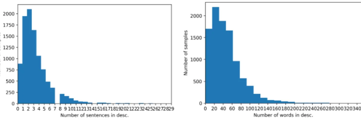
A majority of descriptions have a similar structure to the one above, in that they are 2-3 sentences long and comprise of 20-60 words 3.1.1. Others, however, can be quite varied in both their structure and content.

Figure 3.1.1: Distribution of the number of sentences and words in 10000 randomly sampled descriptions

A significant portion of the data contains very short descriptions, containing < 20 words. Some of these provide a brief, succinct overview of the content of the podcast (for e.g. ’The Wall Street Journals editor in chief, Matt Murray, explains the economic risks and realities of the coronavirus pandemic.’), while others are too vague and do not offer too much information (e.g. ’This is short podcast for my students at Changzhou University. I read a chapter from the book love or money -support this podcast: https://anchor.fm/pat-sauers/support’)

The longer descriptions, on the other hand, always seem provide useful information about the podcast.

3.1.2

Topics

As an initial test, the complete model vocabulary was used as potential topics. This, however, resulted in articles, pronouns and other redundant words like podcast, episode etc. being predicted as labels. To overcome this problem and to allow some control over the predicted labels, a pre-defined set of words was used as potential topics. This also ensured that only those words which are deemed to be good enough as labels (determined by meeting certain criteria) were considered by the model.

Spotify currently makes use of keyword extraction to assign labels. For the project, a subset of all keywords generated via keyword extraction was used as the set of potential topics. From the complete set, only those keywords which were popular, i.e. those that were the keyword for more than a certain number of podcasts, and additionally had a Wikipedia page attached to them, were considered as topics. This resulted

in a total of 103643 distinct topics. Some examples of these topics include : Blue moon, Shower gel, Brothel, Bruise, Brown hair, Meat industry, Webcam model and Chamomile.

3.1.3

Test Set 1: Descriptions assigned with the correct label

This test set was acquired by from user search logs. The data was collected from the user queries that led to users listening to the podcast. More specifically, if an episode was retrieved and listened to from a user search, the episode description was tagged with the user query as the correct label. The main idea behind this test set was to use user queries as ground truth for the descriptions. However, the ’correct labels’ in the set are limited to the set of existing topics (described above). This is because only those topics can be retrieved by the search system.

Owing to confidential company reasons, the set only comprised a total of 817 samples.

3.1.4

Test Set 2: Descriptions with labels from existing model

At Spotify, once keywords are generated for a description, each of the keywords are then assigned a relevance score by an in-house relevance model. This score is a value between of 0 and 1, which determines how relevant a keyword is for a particular description.

This dataset was a collection of the episode descriptions and their most relevant label (highest relevance score), as assessed by the relevance model. Since the test set was used for a manual evaluation task, the size of the set was limited to 100 and only 100 of the most popular episode descriptions were used.

3.1.5

Training and Testing Data

For training the models, a set of 2.3 million episode descriptions was used. This was generated by randomly selecting 10% of all the episode descriptions available. This was done in order to reduce the computational cost of training and with the notion that such a sample would be a reasonable representation of the complete data.

3.2

Implementation

3.2.1

Model Architectures

Two model architectures were used in this study: word2vec [37] and a transformer based. For the word2vec model, both a pre-trained model and models trained in-house on the podcast descriptions were used. Google’s pretrained model contains word vectors for a vocabulary of 3 million words and phrases which were trained on roughly 100 billion words from a Google News dataset. For each word in the vocabulary, the model produces embedding vectors of size 300. The in-house word2vec models were trained on a 2.3 million descriptions. Raw text data was used as input for training the model. An additional pre-processing step of the text by filtering out all stopwords was also tested, but it failed to provide good results. Figure 3.2.1 shows the distribution of 100 randomly sampled words in the embedding space.

Figure 3.2.1: Visualising the word2vec model: t-SNE [35] plot of the embedding space generated by the word2vec model. This model was trained on small set of 10000 descriptions and 100 randomly sampled words were plotted

A few variants of the word2vec model were trained before finalising the parameters of the in-house model. For all variants, some parameters were kept fixed like the min_count (minimum number of times a word has to occur in the corpus for it to be included in the model vocabulary) was set to 1, and the size (dimension of the resultant embedding space) was set to 300 in keeping with the pre-trained model. Since it is an unsupervised task, there was no definitive way to evaluate the different models. The assessment was done based on a manual evaluation of the labels being predicted, and using accuracy of the best predicted label (metric_1 in section 3.3). Both version of

the model: Skip-grams and Continuous-bag-of-words were trained, and the former showed a better performance than the latter. A few window sizes were also tried around the default value of 5 (4,6 and 7), but this did not appear to affect the model performance very much.

For the transformer based model, Google’s pre-trained USE [6] was used (Transformer encoder in 2.5). The sentence encoder produces embedding vectors of size 512 whether the input is words, sentences or whole paragraphs. This was used to produce vectors for all descriptions and topics.

3.2.2

Generating

description vectors

and

topic vectors

In order to assign labels to the descriptions, the first step was to generate description vectors and topic vectors. These refer to the vector representations of the descriptions and topics in the embedding space respectively.

word2vec model:

The descriptions vectors (or topic vectors) were created by computing the centroid of all the words contained in the description (or topic). Preliminary tests revealed that doing so often resulted in topics containing stop-words being over-represented in the predictions. This is most likely due to the high frequency of the stop-words in the descriptions, causing a higher similarity value between them and the topics containing stop-words. To overcome this, the description and topic vectors were weighted with tf-idf. The following is the overview of the steps involved in creating the vectors:

1. Temporary description vectors were generated as described above, and temporary topic vectors were generated by filtering out all stop-words from them.

2. A tf-idf matrix was created using 5000 randomly sampled descriptions. The weight associated with each word was the average of its tf-idf score across all the descriptions it occurs in. This was done, as opposed to creating tf-idf for each word in each description, because generating the tf-idf scores is a very slow process. At evaluation stage, adding the test descriptions to the corpus and computing the tf-idf scores would have been very inefficient. For all words that do not occur in the 5000 descriptions, the tf-idf score was set to maximum of

the scores of the known words. This was based on the idea that such words are at least as rare as any of the known words and was based on the method proposed in1_.

3. The description and topic vectors were then weighted with the tf-idf scores to create the final embedding vectors.

USE:

The sentence encoder can handle words, sentences and paragraphs as input. The raw text data (descriptions and topics) were used as input to the USE and the produced embeddings were used as is without any post processing.

3.2.3

Assigning Labels

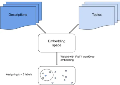
Once all the description vectors and topic vectors were generated, these were used to assign labels to the descriptions based on the distribution of the vectors in the embedding space. k-nearest neighbour was employed to do this. In the embedding space, for each description vector the k nearest topic vectors were computed to assign k labels. Figure 3.2.2 shows the different steps involved in the process. These steps are the same for both word2vec model and USE, with the word2vec having an additional step of weighting with tf-idf.

3.3

Evaluation

As discussed in section 1, assessing relevance of topics associated with texts can be challenging for a multitude of reasons. For this project, the quality of the labels was evaluated both quantitatively and qualitatively. The initial stages of the project involved more of a manual assessment of the labels generated by the models. This led to the incorporation of tf-idf while generating the vectors.

For the quantitative tests, the accuracy of the predicted labels was computed by comparing them to the existing labels (Test Set 1 from section 3.1). Two evaluation metrics were used for this purpose. The percentage of samples where the best

1_{http://nadbordrozd.github.io/blog/2016/05/20/text-classification-with-word2vec/. Accessed:}

Figure 3.2.2: Steps involved in generating description and topic vectors.

prediction of the model matched the existing label was our first metric. That is:

metric_1 = ( ∑n

i=11predictedi=correcti)× 100 n

For our second metric, we looked at the percentage of samples where one of the top three labels predicted by our models matched with the existing label.

metric_2 = ( ∑n

i=11correcti∈top3_predictedi)× 100 n

Here, 1 is the indicator function, predictedi is the model prediction for ith sample,

top3_predictediis the set of top three predictions made by the model for the ithsample,

correctiis the correct label for the ithsample and n is the total number of samples.

Qualitative assessment was done by manually scoring the relevance of the predicted topics. For this, three participants (two thesis students and one employee at Spotify) were asked look at the podcast descriptions and the labels predicted by the different models, and judge them as relevant or irrelevant (1 or 0 respectively). We then evaluated the performance of our models by calculating the mean of the number of

times they deemed it as relevant. That is ∑n

i=1relevancei

n

Results

This section describes the tests that were conducted and their results. The four datasets described in section 3.1 were used for these experiments. The results are followed by an analysis of the errors.

4.1

Accuracy with Keyword Extraction

To test accuracy of keyword extraction, a subset of Test Set 1 (section 3.1.3) was used as the evaluation set. As mentioned in section 3.1, the labels associated with each description in this test set were considered ground-truth for the evaluation. One problem, however, was that in more than 90% of the samples the text did not contain the assigned label. For a more accurate evaluation of the model, all the samples which did not include the label in the text were removed (based on the method suggested in [53]). This resulted in a total of 73 test samples.

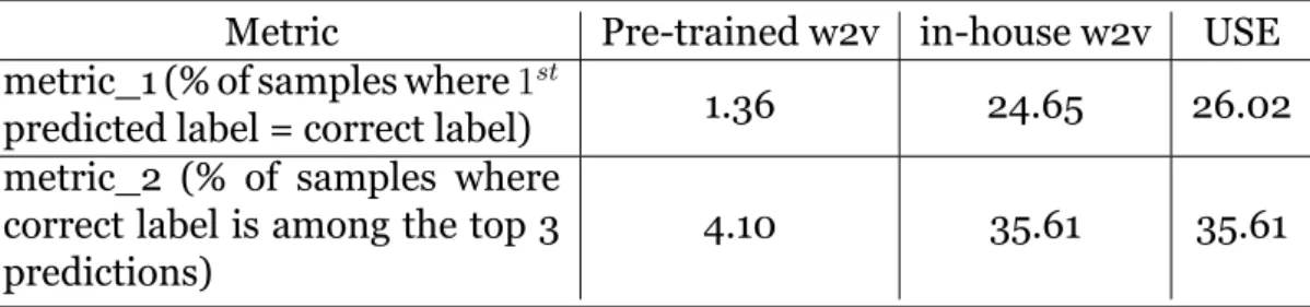
Table 4.1.1 shows the performance of the three models at keyword extraction task based of metric_1 and metric_2, as described in section 3.3. As can be seen, both the in-house word2vec and USE significantly outperform the pre-trained word2vec model. It should be noted that the performance of the USE is only slightly better than that of the in-house word2vec model.

The pre-trained word2vec model performs very poorly at this task. This could potentially be because the sample size is very small, and podcasts pertaining to one field, Real Estate, are over represented in the test set with about 23% being about this

subject matter.

Although the objective of the thesis project was to move beyond a simplistic keyword extraction approach, this test provides a basic understanding of the quality of embeddings generated by the different models with regards the podcast description dataset.

Table 4.1.1: Performance of the three models at keyword extraction task Metric Pre-trained w2v in-house w2v USE metric_1 (% of samples where 1st

predicted label = correct label) 1.36 24.65 26.02 metric_2 (% of samples where

correct label is among the top 3 predictions)

4.10 35.61 35.61

To validate the significance of these results, we conducted Chi-square tests that led to the following results:

• The in-house word2vec outperformed the pre-trained word2vec in terms of both metrics (p < 0.0001).

• The USE outperformed the pre-trained word2vec in terms of both metrics (p < 0.0001).

• The difference in performance of the USE and the in-house word2vec, however, was not significant.

4.2

Overall Accuracy

To test the overall accuracy achieved by the three models, all the samples from Test Set 1 (section 3.1.3) were used, containing a total of 817 samples. The correct labels in this test case were not necessarily words explicitly mentioned in the text, and so the models are evaluated based on how well they are able to predict context dependent labels. Therefore, doing this test provides us an understanding of how well the models are able to learn the meaning of the text and the semantic relationship between words.

Table 4.2.1 shows the performance of the three models based on metric_1 and metric_2 (section 3.3). As can be seen, USE demonstrates a better performance than both

word2vec models. Interestingly, unlike the previous test, the pre-trained word2vec model outperforms the in-house word2vec model here.

Table 4.2.1: Overall accuracy obtained by the three models

Metric Pre-trained w2v in-house w2v USE metric_1 (% of samples where 1st

predicted label = correct label) 11.50 5.01 15.54 metric_2 (% of samples where

correct label is among the top 3 predictions)

17.13 7.34 23.25

As with the previous test, Chi-square test was conducted to assess the significance of the results:

• The pre-trained word2vec outperformed the in-house word2vec in terms of both metrics (p < 0.0001).

• The USE outperformed the pre-trained word2vec (p < 0.05 for metric_1 and p < 0.01 for metric_2).

• The USE outperformed the in-house word2vec (p < 0.0001 for metric_1 and p < 0.05 for metric_2).

4.3

Comparing with existing model

As discussed in section 1, relevance of labels is dependent on a variety of factors, and is heavily influenced by the context and users’ point of view. In order to evaluate the quality of the predictions made by the models, it was vital to conduct a manual assessment of these predictions.

For the manual evaluation test, Test Set 2 (section 3.1.4) was used and scoring was based on the method described in section 3.3. For the 100 test samples, the current labels, and labels predicted by the in-house word2vec and USE were examined. The participants were asked to score the labels as 1 or 0 (relevant or irrelevant, respectively) depending on whether they thought it was a relevant label for the podcast description. The table 4.3.1 shows the percentage of samples that were classified as relevant by the participants. Although USE achieves a higher score than the word2vec model, it is lower than the score achieved by the current labels.

Table 4.3.1: Mean Relevance scoring obtained by the predictions of the different models. Here, 1st_{, 2}nd _{and 3}rd_{refer to the 1}st_{, 2}nd _{and 3}rd_{label predicted by the model.}

Current model in-house w2v USE 1st ₂nd ₃rd ₁st ₂nd ₃rd

61.1 8.23 5.8 8.23 27 22.35 17.6

In order to validate the significance of the results of this test, a Chi-square test was conducted. To do this, the distribution of the 1st _{predicted label of the in-house}

word2vec model was compared against the distribution of the 1st _{label of the USE,}

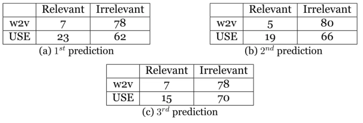
and similarly for the 2nd _{and 3}rd_{prediction. Table 4.3.2 shows the contingency tables}

used for the Chi-square test. In all three cases, the null hypothesis was that there is no relation between the two variables: the model that is being used and the relevance score.

Table 4.3.2: Contingency tables associated with the three distributions Relevant Irrelevant w2v 7 78 USE 23 62 (a) 1st_prediction Relevant Irrelevant w2v 5 80 USE 19 66 (b) 2nd_prediction Relevant Irrelevant w2v 7 78 USE 15 70 (c) 3rd_prediction

• The 1st _{prediction (table 4.3.2 (a)), resulted in a chi-square statistic of 10.3619}

and a p-value of .001286 (< 0.01). This implies the result is significant at p < .01 • The 2nd _{prediction (table 4.3.2 (b)), resulted in a chi-square statistic of 9.5091}

and a p-value of .002045 (< 0.01). This implies the result is significant at p < .01 • The 3rd_{prediction (table 4.3.2 (c)), resulted in a chi-square statistic of 3.3415 and}

a p-value of .067552 (> 0.01). This implies the result is not significant at p < .01. These tests showed that there was a significant difference between the performance of the in-house word2vec and USE when it came to comparing the relevance of the 1st

and 2nd _{prediction, but not the 3}rd_{one. Although, this means we cannot definitively}

rank the performance of the models, we can conclude that in terms of the models’ best prediction, the USE outperform the in-house word2vec.

This method of evaluation, however, poses a problem. Since the current model is based on keyword extraction, the current labels are always explicitly mentioned in the description, making it easy to assess its relevance. With the sentence encoder and the word2vec models, sometimes the relevance of the predictions is ambiguous or requires more knowledge about the contents of the podcasts to make a judgement.

It is easy to see that this method of assessment favours the existing labels. Though this test provides an understanding of how the different models perform, they are biased ways of evaluating the models.

4.4

Error Analysis and Discussion

This section provides an overview of some of the common errors in the USE predictions and their possible reasons. Additionally, possible solutions or workarounds to these errors are also discussed. Following this, a discussion about the results obtained by the different models is presented.

4.4.1

USE

error analysis

1. Short Descriptions

The dataset contains several short descriptions (figure 3.1.1), i.e. descriptions that made up of one sentence and/or contain ∼ 20 words. Some of these are succinct descriptors and do a sufficiently good job at capturing the context of the podcast (eg. ’Roslyn speaks on the subject of SELF COMFORT shares simple steps to explore and tap into one’s self. Being yourself is extremely important. Press play to hear her pHERspective as to why’). These generally work as good input for the models and produce good labels. On the other hand, there are some descriptions which, apart from being very short, are also vague. These often contains website URLs, words like ’subscribe to’, ’follow more at ..’ etc. and do not contain enough information to produce good labels. Given below is one such example.

Example

Description: This is short podcast for my students at

money --- Support this podcast:

https://anchor.fm/pat-sauers/support,c3bc12a9-2947-4c88-ae22-5f2ced58f218

Correct label: Business English

1st predicted label: Soundings Podcast (0.53673434) 2nd predicted label: Podcast (0.5265429)

3rd predicted label: A Very Spatial Podcast (0.51254237)

In this example, there is very little text in the description that can be picked up by the model ’relevant’ and hence, it ends up generating redundant labels. Even if the labelling were to be done manually, assigning labels to such texts could prove to be challenging.

When distilling all the content in the podcasts into summaries, some amount of information loss is unavoidable. Further compressing these to generate labels increases this loss, and some valuable or relevant content is bound to be lost. Using texts that provide very little information as input to the model, almost guarantees bad quality labels.

One possible workaround to this problem could be by enhancing the information provided in these descriptions, by looking at the corresponding show description (also provided by the content creators at the time of publishing podcasts on Spotify) or the entire transcript of the podcast, and thereby allowing the model to leverage a wider information source.

2. Instances where the correct label is a proper noun (often names of people)

Example

description : on this special episode of on purpose, i got to sit down with my good friend gary vee. gary is an investor, a serial entrepreneur and a 5 time new york times bestselling author. we got to talk in depth about how to stop caring what people think about you, why you should focus on happiness not hustle and why you need to contextualize advice before you

decide to listen to it. there are so many teachable moments in this episode and i know you will learn so much!

correct label : Gary Vaynerchuk 1st : Gary Chartier (0.38306186) 2nd : Gary Gerould (0.36270785) 3rd : Gary Burghoff (0.3587864)

In several cases where the correct label is the name of a person, the models (for USE and the word2vec) are prone to errors. Some of the errors include only getting a part of the name right (example above) or predicting only one name when multiple names are mentioned in the text. These errors can be handled by assessing what qualifies as a separate topic entity and what doesn’t.

In the example above, the model predicting Gary Chartier/ Gerould/ Burghoff instead of Gary Vaynerchuk, a name neither explicitly mentioned in the text nor well known enough for most people to automatically associate with the context of the description, is a very understandable error. This is a problem stemming from what is deemed good enough to be a topic on its own i.e. what is included in the Topic list, and also the possible use case of such a topic assigning system.

In several instances, including the one mentioned above, none of the predicted or the correct labels make for very good topics, but are assigned merely because they are included in the topic list. When making a list of possible topics, a thorough assessment of what can be considered a good (or relevant) topic is required.

In such a context (example above) the name is not really relevant enough to be a topic on it’s own. Other names such as ’Gandhi’, ’Buddha’, ’Trump’ are more relevant and require a topic entity on their own.

This requires a pre-processing of the topic names and depends on what we want out of the model. Here, the names of the host and guest is a relevant feature to extract but not a very useful topic. This error could be handled by extracting the names of the host and the guest, and excluding them from list of topics for the podcast in question. Additionally, the topic list used to predict labels can be scrutinised more carefully, and only those words which we potentially want as

topics can be included in it. While using the existence of Wikipedia a page and a count based metric to qualify words as potential topics is reasonably good, it probably allows in more words than we want.

3. Returning very similar or related words

Example

description :Matt Templeton got an early start in real estate as an assistant. At age 18, he had his license and was

already selling homes. Fast forward to 2020, Matt now has two teams dominating two different markets and is a true Real Estate Rockstar. On today’s podcast, Matt shares what helped him succeed as an agent, how he built two successful teams, and a follow-up strategy guaranteed to help listeners convert more leads. Sponsors Rebus University – Get Over $10,000 in Real Estate Training for as Little as $97 at

futureofrealestatetraining.com MyOutDesk – Book a FREE Business Strategy Session and See How to Grow Your Business with the Help of a Virtual Assistant at myoutdesk.com FREE Resources for Real Estate Agents Join the FREE Agent Success Toolbox and Get Immediate Access to Over 200 Real Estate Downloads Claim Your FREE Copy of Pat Hiban’s Best-Selling Book: 6 Steps to 7 Figures Claim Your FREE Copy of Tribe of Millionaires by Pat Hiban and David Osborn Learn more about your ad choices. Visit megaphone.fm/adchoices

correct label : real estate

1st : Real estate license (0.3768696) 2nd : Real estate investing (0.37079817) 3rd : Real estate entrepreneur (0.35089764)

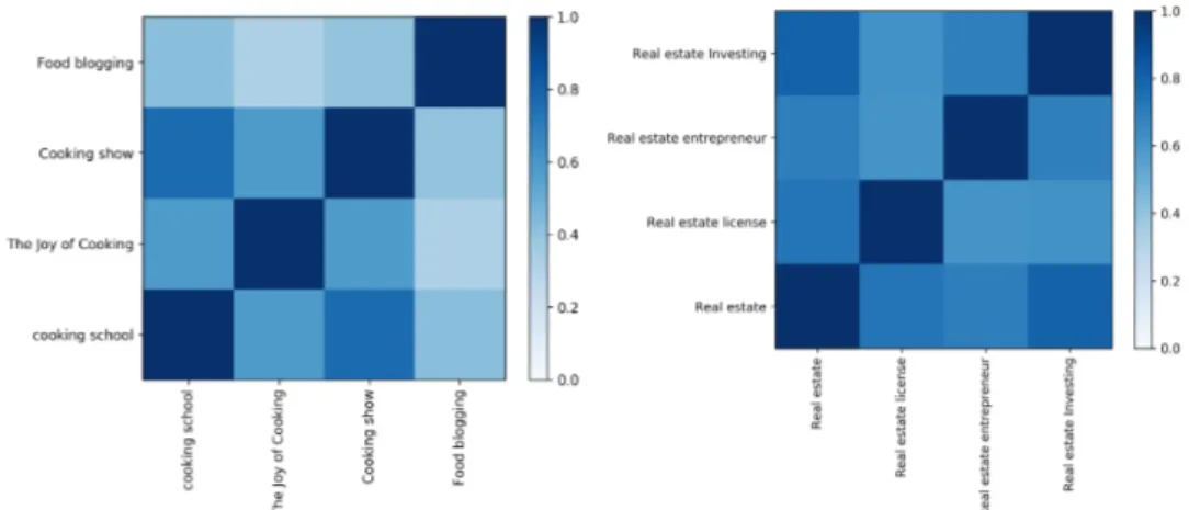
In the example below, the model predicts labels which are very similar to the correct label (figure 4.4.1) but are not exactly the same and hence get marked as an incorrect prediction.

Figure 4.4.1: Similarity scores of the predicted labels and the correct label using embeddings from USE

Example

description : this week�s guest is madalaine mcdaniel, the blogger and youtube host of lakeside table. a channel that is dedicated to showing you how to make simple and tasty recipes each week. a native of saint louis, madalaine was a former medical sales rep, and a single mom that started out cooking by listening out for the fire alarm, however, after meeting her husband jerry, and moving with him and his family to rural illinois, she decided to buckle down and learn to cook. since her early days of humble cooking, madalaine has blogged about her journey become an accomplished home cook in her own right. she now shares what shes learned, as well as tips and tricks about cooking on her show and her blog. in this episode, we talked about midwestern comfort food and amazing authentic italian cuisine, how to elevate dishes with spices, an amazing hack for dried herbs, divinely delicious popovers, the benefits of culinary school education, and a useful trick for measuring cream based foods. you can find madalaine on her website, youtube, instagram, pinterest, and facebook recipes mentioned in this episode popovers pecan crusted salmon over mustard sauce chicken tortilla soup golden crusted crab cakes come visit bff with the chef: the bff with the chef website twitter facebook instagram

correct label : cooking school

1st : The Joy of Cooking (0.3614062) 2nd : Cooking show (0.35326898) 3rd : Food blogging (0.3516994)

’Joy of Cooking’ (name of a book) is an irrelevant prediction and it does not have much to do with the content of the description. This is a very obvious error made by the model, but as with any DL model, some amount of error should be expected. The other two predictions, descpite not being correct, are relevant with ’Food blogging’ being arguably more relevant than the correct one itself.

In both examples, the model predictions add no value to the accuracy score described in the experiments and give no credit to the model. However, these predictions are valuable and can therefore not be classified as errors either. 4. Instances where model prediction is more relevant than

Example

description :last week, cnn broke the story that the united states had secretly extracted a top spy from russia in 2017. what does that mean now for american intelligence operations? guest: julian e. barnes, who covers national security for the new york times. for more information on todayâ��s episode, visit nytimes.com/thedaily.â background reading:â the moscow informant was instrumental to the c.i.a.â��s conclusion that president vladimir v. putin had ordered and orchestrated russiaâ��s election interference campaign.

correct label : cnn

1st : Russian interference in the 2016 United States elections (0.46988517)

2nd : Soviet espionage in the United States (0.4181317) 3rd : KGB (0.39150792)

The label assigned as ’correct’ is clearly wrong in this case. ’CNN’ provides no information about the podcast and is most likely assigned as a label since it is mentioned in the text. The predictions, on the other hand, are all relevant. The

sentence encoder does a good job at using a text and deciphering its content and meaning. Again, as in the precious case, it is very tough to quantitatively assess and compare their relevance.

This error boils down to the testing data that we use as ’gold standard’ to compare predictions to. For a problem such as this one, no dataset is going to be absolutely correct and error free. This problem, as discussed in the introduction, stems from ’relevance’ being highly subject and very dependent on the lens through which we view the results. It is an age old error which has existed right from when labels were manually assigned, where what one deems as relevant might not be so for another. This does not really fall under the category of an error of the model, but more of a shortcoming in the evaluation metric that we have decided.

4.4.2

Difference in performance across models

In some instances, the word2vec models to predict labels which is more reliant on word matching than actual contextual labels, as opposed to the USE, which predicts context dependent labels. This is best encapsulated by the following example:

Example

description : Ever since NASA broadcast its visits to the Moon between 1969 and 1972 to millions of people around the world, conspiracy theorists have debated endlessly over the photographs and video of the journey....after the last Apollo mission,

titled “Conspiracy Theory: Did We Land on the Moon”? Poring over every single detail for inconsistencies and potential government tampering, people who buy into the Moon landing conspiracy theory strive to prove that NASA never went to the moon. .... Some believe that because sending astronauts into outer space and onto the moon would be incredibly expensive, the US did not have enough money to complete the project. According to the conspiracy theorists, faking the Moon landings would be much cheaper – if it were convincing that because sending astronauts into outer space and onto the moon would be incredibly expensive, the US didn’t have enough money to complete

the project. According to the conspiracy theorists, faking the Moon landings would be much cheaper – if it were convincing enough, it could still send a message to Russia that the United States had the better technology. ... To get the answers to these questions and more, Turn On, Tune In Find Out! Correct Label : moon landing conspiracy theories

Predicted Topic names (k = 3) USE:

1st : Moon landing conspiracy theories (0.70455694) 2nd : Moon landing (0.65508926)

3rd : Great Moon Hoax (0.4640981)

pre-trained: 1st : Normandy landings (0.57233147) 2nd : Moon landing (0.45950862) 3rd : Emergency landing (0.45950862) in-house: 1st : Normandy landings (0.71615849) 2nd : Alternative facts (0.39722231) 3rd : Binary-coded decimal (0.39559181)

The USE not only predicts the right label, but also makes use of the context to predict other labels about Moon and conspiracy theories. The pre-trained word2vec model appears to heavily weight the word ’landing’ and predicts labels where the word occurs. The in-house model, evidently predicts completely wrong labels.

Another reason for the superior performance is that the sentence encoder is trained on several transfer learning tasks.