Crack speed in wood fibers composites and PLA

(1)

Department of applied mechanics

Project in Physics and Astronomy

Crack speed in wood fibers composites and PLA

Author: Axelle Aimard

Supervisor: Thomas Joffre

Examiner: Allan Hallgren

(2)

I) Abstract ... 3

II) Introduction ... 3

III) Theory ... 5

IV) Materials and methods ... 13

V) Experiment – Results... 17

VI) Conclusion ... 23

VII) Appendices ... 24

(3)

I)

Abstract

An experimental set up as been developed aiming to use a high-speed camera to measure crack speed propagation. Using this experimental set up the velocity of a crack tip has been measured in different natural fiber composite materials and PLA. The experiments were performed under different humidity conditions (dry and soaked into water) and for different crack length: 10%, 20% and 30% of the plate width. The speed measured ranged from approximately 400 m/s for long cracks in wet samples to approximately 850 m/s for short crack in dry samples. Classical fracture mechanics was able to explain the variations observed due to the crack length when the samples were kept dry. However, in the wet state, the crack speed is in some cases independent on the initial crack length which seems indicate that the crack speed does not depend on the fracture energy. This result might be due to a change in fracture mechanisms at the polymer chain level and highlight the need of new modelling approaches to predict the dynamic failure of heterogeneous materials.

II) Introduction

Fracture is an everyday life problem, the structures around us have to stand, for example. As the technology become more and more complex, the problem of fracture increases.

A lot of study of material's failure have been done since World War II and we are now even able to prevent such phenomena in some cases.

To enhance the knowledge on this topic could contribute to a save of a lot of money. For example, in the United State, the cost for fracture is estimated to be more than a hundred billion of dollar per year, with research it could be reduce by 20 %.

(T.L Anderson, 2005,

[1])

Fracture theory can be applied to different fields, like seismology, this can be explained by the fact that an earthquake is mainly a dynamic crack growth process on a large scale.

In nuclear industry, the study of fractures is also something important, large experiments have been run to investigate the arrest capacities of materials.

(Nilson Fred, 1999, [2])

2.1 Purpose

The purpose of the project is to study the crack propagation in different materials and with different parameters: moisture, initial crack length and fibers modifications.

The materials studied will be PLA and wood fibers composites.

A sample with an initial crack will undergo a tensile test, and the propagation of the crack will be recorded with a high-speed camera.

(4)

2.2 Background

2.2.1 High-speed camera:

The possibilities offered by a high-speed camera are numerous. For example, Researchers from the MIT Media Lab have created a new imaging system that can acquire data at a rate of one trillion frames per second (fps). At this velocity, light traveling through objects can be recorded.

(MIT media lab, 2011, [3])

2.2.2 Shear wave:

In fracture theory waves propagating in materials are considered to be the limited speeds for crack propagation, however a study made by AJ Rosakis showed that in a brittle polyester resin, the shears crack can propagate at higher speeds than the shear wave speed.

(Rosakis

A.J, 1999, [4])

2.2.3 Crack velocity & branching:

First researchers such as Sharon & al were looking at the fracture pattern

(Sharon &

Al,1995, [5])

but with the development of high speed camera, scientists were able to estimate the crack speed in strengthened glass and polymers.

Tang Zhongzhi & al studied strengthened glass. They used a high-speed camera which recorded 500,000 fps. They found the crack speed in glass to be around 1700 m/s.

(Tang,

Zhongzhi, et al.2014, [6]).

Kazuo Arakawa & al were looking at different polymers: the araldite and the homalite. By using a high-speed camera, they studied the branching phenomena but also the crack velocity and the stress intensity factor.

For the homalite, they found a velocity between 300 and 425 m/s for an initial crack length1 between 0,1 and 0,3.

For the epoxy, they found a velocity between 260 and 300 m/s for an initial crack length between 0,1 and 0,3.

(Arakawa, Kazuo, and Kiyoshi Takahashi,1991, [7])

2.3 Sample studied:

Wood fibers composites have many applications: they can be used for example for car parts. They have several advantages over synthetic fibre composites, for example the fibers are lighter and natural. The most common wood fiber composite has polyethylene (PE) matrix because of the price.

The samples we will study are wood fibers composites with a polylactic acid matrix (PLA). PLA is more expensive than PE but permits to have better mechanical proprieties.

This can be explained by the fact that wood fibres are hydrophilic and the polymer matrix is hydrophobic. The poor affinity between the fibers and the matrix results in the agglomeration of the fibers

(Balasuriya et al., 2001; Joffre et al. 2014b, [8])

and a lower stress transfer ability at the fibre-matrix interface. The PLA matrix is less hydrophobic than the PE matrix so

those two phenomena are less important with PLA resulting in better mechanical proprieties.

(Joffre, Thomas, et al.,2016, [9])

(5)

III) Theory

3.1 Crack mechanics

3.1.1 Crack separation modes:

Figure 1.Different fracture modes [1]

Mode I: Opening mode

In this mode, the tensile stress is normal to the plane of the crack. This mode is the most important mode since mode II cracks tend to re-orient in mode I. That’s the mode we will study.

Mode II: Sliding mode

In this mode, the shear stress acts parallel to the plane of the crack and is perpendicular to the crack front.

Mode III: tearing mode

In this mode, the shear stress acts parallel to the plane of the crack and also parallel to the crack front

.

(David Roylance, 2001, [10])

3.1.2 Griffith’s model:

Griffith's model is based on the change of energy during the growth of a crack. It shows that the crack propagation is due to a transfer of energy, this model is valid for infinite plates of brittle homogenous and isotropic materials.

In this study, the plates studied are considered to be infinite.

(6)

In this model, we are considering a slab with a central crack which has a length of 2a, this slab is subjected to a uniform tensile stress σ, at infinity.

Griffith demonstrated that the crack will propagate when the available elastic strain energy is at least equal to the energy needed to create new crack surface.

To create a new crack surface the stress needed is equal to:

(1)

where E is Young's modulus (Pa), ɣ is the surface energy of the material and a is the crack's length (m).

(2)

G is the energy release rate (Pa.m) or fracture energy.

(Fred Nilson, 1999, [2])

3.2 Determination of the fracture energy:

By doing a tensile test the force applied and the stroke will be recorded at the crack initiation. Using those data, the stress and the strain will be calculated.

The stress is link to the force as following:

(3)

Where σ is the stress, F is the force at the crack initiation, w is the length of the specimen and t is the thickness of the plate.

Then the fracture energy will be determined:

(4) Where G is the fracture energy, σ is the stress at crack initiation, a is the initial crack length, and E is the elastic modulus.

(Fred Nilson, 1999, [2])

σ=

√

2 E γ Πa

G=2 γ

σ=

F

wt

G=σ 2_{Π a} E

(7)

3.3 Evolution of the fracture energy with the velocity

Illustration 1.Velocity functions for gamma [3]

As we can see in Illustration 1, in theory, according to the text book by Fred Nilson the fracture energy should increases exponentially with the velocity. This is due to the fact that when the initial crack is small there is more energy to release.

(Fred Nilson, 1999, [2])

Note: In illustration 1, the x axis represents the crack velocity divided by the speed of the shear wave and the y axis represents the normalized fracture energy.

3.4 Shear, pressure and Rayleigh waves:

3.4.1 Shear waves

Shear waves are elastic transversal waves, meaning that the motion is perpendicular to the direction of the propagation of the wave. They are not divergent, and obey the continuity equation for incompressible media.

(5)

Where Cs is the speed of the shear wave propagation (m/s), υ is Poisson’s ratio, E is Young's Modulus (Pa) and ρ is the density (kg/m

ᵌ

). (Priestley Keith ,1999, [11])

3.4.2 Pressure waves

Pressure waves are longitudinal elastic waves, the motion has the same direction as the direction of propagation of the wave.

(6)

Where Cp is the speed of the pressure wave propagation (m/s), E is Young's Modulus (Pa) and ρ is the density (kg/m

ᵌ

).

(Milsom Jhon,Field ,2003,[12]).

Cs=

√

E

2∗(1+υ)∗ρ

(8)

3.4.3 Rayleigh waves

Continuum mechanics theories suggested that Rayleigh velocity should be the limiting crack tip velocity, Rayleigh speed wave propagation can be approximated by:

(7)

(Mott Nevill Francis,1948, [13])

3.5 Crack propagation

In theory, the crack tip velocity should approach, but never exceed the Rayleigh velocity. However, crack velocities close to the Rayleigh velocity have only been observed once by Rosakis et. al. 1999. Otherwise experiments by Nilsson (1972, 1974,

[21

]), and Ravi-Chandlar et. al. (1984),

[14]

report a maximum crack speeds of 0.4 − 0.8Cr.

Investigations of the fractured surfaces typically shows so-called mirror-mist-hackle patterns (

Sharon et. al. 1999, [15]

).

At the beginning, the crack propagates slowly and leaves a mirror-like surface. When the crack accelerates, it turns misty, and becomes at the end tortuous (hackle).

An experimental study ran by Fineberg et. al. (1991) showed that crack propagation at velocities over 0.4Cr is unstable for homogenous materials. (

Fineberg et. al,1991, [16]

). This instability results in microscopic branching, which can be observed as the hackle pattern on the fracture surface (

Sharon et. al.,1995, [5]

).

The results obtained by Fineberg and Sharon support the crack branching mechanism

suggested by Ravi-Chandlar et. al. in 1984, this macroscopic branching is due to microscopic cracks in front of the crack tip. The area in front of the crack in which microscopic cracks are formed is called the process zone.

Numerical simulation will later confirm the mechanism suggested by Ravi-Chandler (

Bobaru

et. Al, 2015 and Murphy et. Al, 2006, [17]).

Bobaru & al and Murphy both conclude that crack bifurcation is preceded by a widening of the fracture process zone.

Cr=Cs∗[0,862+1,14∗ν 1+ν ]=

√

E 2∗ρ∗[1+ν ]∗[ 0,862 +1,14∗ν 1+ν ]

(9)

3.6 Evolution of the velocity with the crack length

The relation between velocity and crack length has been determined by Anderson applying a dimensional analysis to a propagating crack. This applies for an infinite plate.

He determined the relation between the kinetic energy and the crack speed.

(T.L Anderson,

2005, [1])

(8) Where Ek is the kinetic energy (J), k is a constant which depend on the material, ρ is the density (kg/m3), a is the crack length (m), V is the velocity (m/s), σ is the stress (Pa), and E is Young’s Modulus (Pa).

Applying Griffith’s model, the fracture energy G is defined as following:

(9)

Where w is the work of fracture (J) and equal to the surface energy in the limit of an ideally brittle material, and k is a constant.

When the crack is initiated the kinetic energy term is not present meaning that :

(10)

By substituting, V is obtained to be :

(11)

Where Cp is the pressure wave (m/s), ao is the initial crack length (m) and a is the total length of the crack (m).

With this relation, we can see that in theory the velocity should be higher when the initial crack is small.

(T.L Anderson, 2005, [1])

Ek =0,5∗k∗ρ∗a2∗V2∗[ σ E] 2 G=0,5* [Π * σ * a 2 E − k2* ρ* a 2 * V2* [σ E] 2 ]'=2 w a o=2 * E * w Π σ2

V =

√

2∗Π

k

∗Cp∗[1− ao

a

]

(10)

3.7 High speed camera

3.7.1 History of high speed camera

The history of high frame imaging began in the 19th century, with the photographer Eadweard Muybridge. By using a sequence of still cameras he photographed moving horses.

(Kris

Balch, 1999, [18])

Illustration 2. Sequence made by Eadweard Muybridge [4]

3.7.2 What is a high-speed camera?

A high-speed camera is a camera which is able to record more than 1,000 frames per second. A common camera is recording between 24 and 40 frames per second.

Today the fastest high speed camera can record a trillion frames per second.

(MIT media lab,

2011, [3])

3.7.3 Applications

High speed cameras have a large range of applications. It can be used for scientific usage to study things not visible with the eyes: fluid mechanics, water droplet, live cells functioning... There are also industrial applications and military application, for example high speed camera can be used in production and assembly lines for industry in order to better tune the machine or for ballistics in military application. (

Kris Balch, 1999, [18]

)

3.7.4 Different types of high speed cameras:

At first, high speed cameras used films to record, until 1960 it was the only device available. Nowadays, most of the high-speed cameras are using electronics devices: CCD or CMOS sensors. Electronics is more efficient because with films camera you need a wind-up time to get to full speed while electronic camera can be triggered automatically, and record

(11)

3.7.5 Functioning

Imaging device: CCD and CMOS sensors

CCD means charge-coupled device and CMOS complementary metal-oxide semiconductor.

The first CCD sensor was developed in 1970 and the first CMOS in 1980.

The sensors convert the light signal (photons) into an electric signal (electrons) using photo sensible cells that recovered them.

(Photovore, 2011, [20])

3.7.6 CCD's functioning:

Illustration 3. CCD's sensors [5]

CCD's are composed of a field of light-sensitive small cells which are commonly called pixels. Each cell accumulates the light (photons) and converts it into electrons. The number of electrons is proportional to the intensity. The intensity received by each cell will be used to determine the colour at each pixel. A Bayer analogic filter will be used to convert intensity into colour.

(Photovore, 2011, [20])

3.7.8 CMOS' functioning:

CMOS’ sensors use a field of photodiodes. Each photodiode is sensible to only one of the primary colour (red, green, blue). There is only two possible answers « yes » or « no » converted in 1 or 0. By combining all the values from the different photodiodes the colour of each pixel can be obtained.

(Photovore, 2011, [20])

(12)

3.7.9 Comparison of CCD and CMOS sensors

CCD

CMOS

Image

High quality, low-noise

Low quality, High noise

Price

++

+

Light sensibility

High

Low

Power needed

++ (100x more than CMOS)

+

Usage

Older : more pixels

New

Battery life

+

++

table 1. differences between CCD and CMOS

3.7.10 Signal processing:

Illustration 5. Functioning of signal processing

At first, the signal from the sensor is sent to a preamp that will amplify the signal. Then, the signal will be sent to a sample and hold circuit. It's an analog device that captures the signal of a varying analog signal and holds its value for conversion. The next step is to convert the analog signal into a digital value, this will be done by the analog-to-digital converter. In general, pixels values are converted to 8 bits. (

Kris Balch,1999, [18])

3.7.11 High speed camera used in the experiment

The high-speed camera used for recording the crack velocity is a motion pro Y8-S2.

The maximum resolution is 1600 * 1200.Therorically, the max frame rate is 165 000 fps and at this rate the recording can last 3,84 s with a resolution of 1600x16. This camera is

composed of a CMOS-Polaris II sensor.

(13)

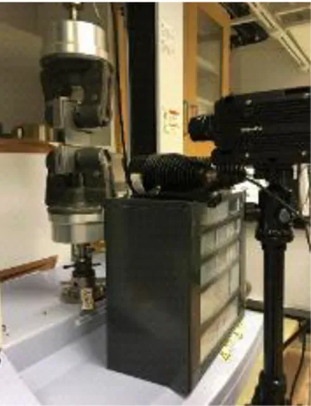
IV) Materials and methods

4.1 Experimental setup - Camera triggering

The camera can be triggered either manually or by motion. Motion trigger:

The camera can be triggered automatically if there is a motion in the image, meaning that a change in contrast in the image is necessary to trigger.

We did preliminary test with the motion trigger. In order to have a high contrast when the light get through the crack, samples were painted in black and light was put behind.

With this setup, the higher number of fps available was 30 000fps. It wasn’t enough to track the crack speed. Indeed, if the number of fps is increased, then the exposure decreased so much that more lights need to be added. Then the motion trigger is not functioning anymore because the variation of light intensity is too high. Furthermore, there is a time difference when the light get through the crack and when the crack is actually moving. The velocity measured using this technic would have been lower than the real value.

Manual trigger:

The camera can be triggered manually, by doing that, the variation of the light intensity is not a problem anymore so it permits to have a higher number of fps.

The numbers of frame per second, the exposure and the resolution are linked all together. The problem of the exposure is solved by adding more lights but, a compromise has to be found for the number of fps and the resolution knowing that the maximum frame rate of the camera is inversely proportional to the number of rows in the region of interest

.

The samples we are studying are 10cm long and 5cm large, meaning that we had to have a large region of interest. The camera is recording continuously, so we can record the time before the camera is

triggered.

(14)

4.2 Manufacturing

In this study, we used wood-fiber plastic composites samples and PLA (NatureWorks Ingeo 3251D) samples.

The composites are composed of softwood CTMP fibres (CS770, Rottneros, Sweden). Part of the fibres have been acetylated in order to increase the mechanical proprieties. The fibers have been acetylated in 50g batches. For 4h, the fibres were oven dried and boiled in acetic anhydride in a 1-L glass reactor.

The PLA and the fibers (unmodified and acetylated) were compounded using a co-rotating twin screw extruder (Coperion ZSK 26K, 10.6, Coperion, Germany) and granulated. Then the granules were injection moulded into plates with the following dimensions: 1*100*100 mm

ᵌ

. The fiber/polymer ratio is 20/80 for all the materials.

Different kind of samples have been realized changing the ratio between modified and

unmodified fibres: 100% modified fibres, 75 % modified fibres, 25% modified fibres.

(Joffre,

Thomas, et al,2016, [9])

4.3 Mechanical Testing

Rectangular samples of 100*50*1 mm were cut using a saw. Cracks were made in the samples using a saw and a razor blade. The razor blade was used in order to have a better crack. We cut all the samples in the injection direction.

Three crack length ratio (a/w) were studied: 0,1, 0,2 and 0,3. Some of the samples have been soaked in water during 5 days, which is the time necessary to be in the equilibrium conditions. During this process, the temperature was constant.The samples stayed into the controlled environment until the experiment.

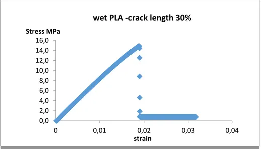
For the experiment, we used a Shimadzu Ags-X at a cross head speed of 5mm/min. The force sensor was 10 kN. The clamps used were 11cm long and were using hydrostatic pressure. The software used for the data acquisition is Trapezeimux, which gives the time, the force and the stroke.

For each sample, we calculated the stress and the strain and draw the curves stress versus strain in order to make sure that the conditions of the test were good. (no slip for example)

Figure 3. example of stress versus strain curve

0,0 2,0 4,0 6,0 8,0 10,0 12,0 14,0 16,0 0 0,01 0,02 0,03 0,04 Stress MPa strain

(15)

4.4 Imaging:

In order to record the propagation of the crack the velocity of acquisition was 69989 frames per second and the resolution 544*64 pixels.

The software used was motion studio. The camera was triggered manually and the acquisition time was 1,7 s with 1,1 s before the trigger.

4.5 Image Analysis:

The image analysis was done manually by using the software fiji

. (a), (b).

On each image, we determined the X and Y positions. Only the X position was used to calculate the velocity. When there were bifurcations, the longest bifurcation was the one used to determine the position.

Knowing the number of frames per second we determined the time for each frame, and knowing the resolution we determined the size of a pixel.

(Appendix 1)

The velocity is linked to the distance and time by:

V=

∆x/∆t

(12)

Where Δx is the distance between two positions of the crack tip, and Δt the time to travel this distance.

We draw the graph of the distance versus the time for each sample, the slope being the velocity.

Figure 4.Example of graph used for the determination of the velocity

R² = 0,9996 0 0,01 0,02 0,03 0,04 0,05 0,06 0,07 0,08

0,00E+00 1,00E-05 2,00E-05 3,00E-05 4,00E-05 5,00E-05 6,00E-05 7,00E-05 8,00E-05 ∆x (m)

t (s) dry composite - crack length 10%

(16)

4.6 Accuracy

We estimated the accuracy on X to be ± 1 pixel equivalent to 0,23 mm (Dx).

The accuracy on the time is 0,015% (Dt), it's the value given by the constructor, there is no way to validate this value.

(13)

We calculated the accuracy on the velocity (DV), using the equation (13). The accuracy varies with the number of points available to calculate the velocity, the maximal error found is 1,3% and the minimum is 0,3%. The measurement is precise, so in the following plot the errors bars won’t be put.

However, all the samples are not the same since they are not produced by an industrial process but manually, so that can explain the variation of velocities between two different samples. Furthermore, others errors could be attributed to the experimental setup.

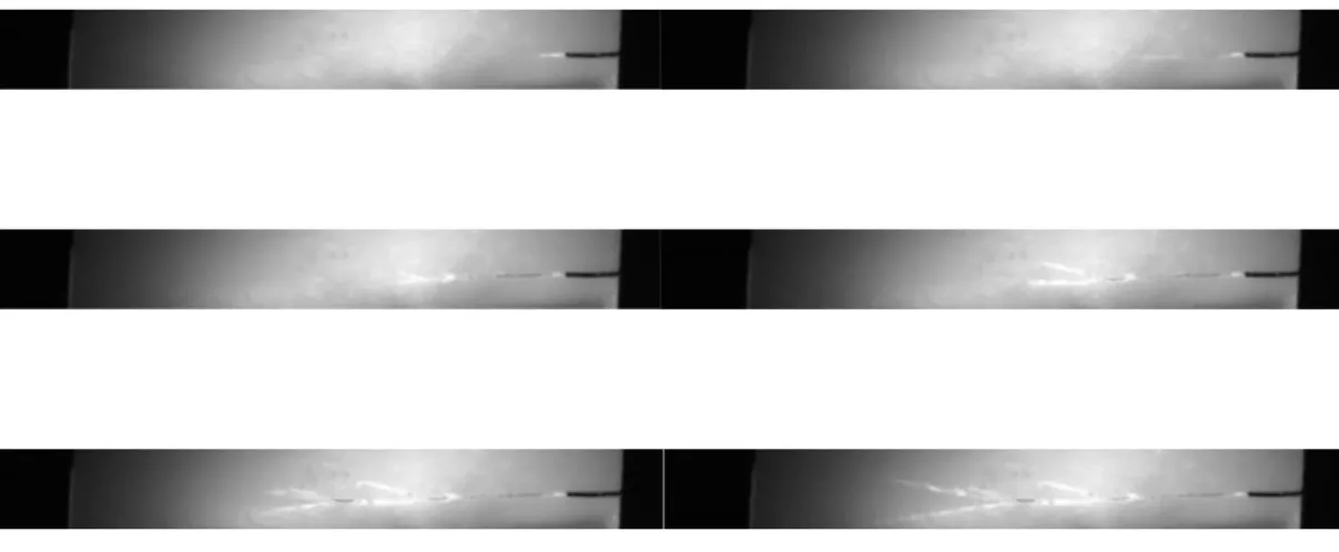
Illustration 8. Example of images’ sequence for the determination of the velocity2

2_{In illustration 8 is shown the propagation of the crack in a sample with an initial crack length} of 1cm. The time interval between each image is 1,43.10^-5 s.

(17)

V) Experiment – Results

5.1 Determination of theoretical values for pressure, shear and

Rayleigh waves:

The shear wave, the pressure wave and the Rayleigh wave theoretical velocities were calculated using formulas (5), (6), (7).

All the velocities are related to the density. The density is equal to the mass divided by the volume. To determine the density, we weighed the samples, and measured the length, the width and the thickness. All the measurement results can be found in Appendix 4.

The velocities are also related to Young Modulus and poison’s ratio. The determination of Young Modulus can be found in Appendix 2 and the values in Appendix 4. The values for poison’s ratio were taken from a previous study on the samples.

In theory, the velocity should be higher in the composites than in the PLA, since the waves’ velocities are higher for composites than PLA.

The velocity is higher when the samples are dry than when there are wet because Young’s Modulus is higher for the dry samples.

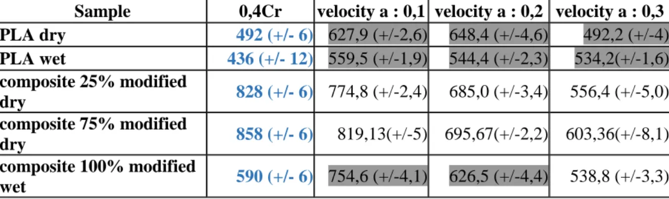
5.2 Determination of branching phenomena

If the velocity is higher than 0,4Cr the crack is assumed to be unstable and branching should appear.

Sample

0,4Cr

velocity a : 0,1 velocity a : 0,2 velocity a : 0,3

PLA dry

492 (+/- 6)

627,9 (+/-2,6)

648,4 (+/-4,6)

492,2 (+/-4)

PLA wet

436 (+/- 12)

559,5 (+/-1,9)

544,4 (+/-2,3)

534,2(+/-1,6)

composite 25% modified

dry

828 (+/- 6)

774,8 (+/-2,4)

685,0 (+/-3,4)

556,4 (+/-5,0)

composite 75% modified

dry

858 (+/- 6)

819,13(+/-5) 695,67(+/-2,2) 603,36(+/-8,1)

composite 100% modified

wet

590 (+/- 6)

754,6 (+/-4,1)

626,5 (+/-4,4)

538,8 (+/-3,3)

table 3. comparison 0,4Cr and crack velocities

Sample

Cp pressure wave (m/s) Cs shear wave (m/s) Cr Rayleigh wave (m/s)

PLA dry

1101 (+/-10)

683 (+/- 8)

1231 (+/- 10)

PLA wet

976 (+/- 18)

605 (+/- 14)

1091 (+/- 19)

25% modified

1851 (+/- 9)

1148 (+/- 7)

2070 (+/- 10)

75% modified

1918 (+/- 9)

1190 (+/- 7)

2145 (+/- 10)

100% modified

1318 (+/- 9)

818 (+/- 7)

1474 (+/- 10)

(18)

Number = branching should appear

5.3 Samples

Dry composite 25% modified

Crack length 0,1 Crack length 0,2 Crack length 0,3

Wet composites 100 % modified

Crack length 0,1 Crack length 0,2 Crack length 0,3

Dry PLA

Crack length 0,1 Crack length 0,2 Crack length 0,3

(19)

Crack length 0,1 Crack length 0,2 Crack length 0,3

5.4 Test 1 – 75% modified fibers composites dry

Velocities:

In figure 5 the crack speed determined experimentally is plotted versus the initial crack length. The speed is seen to be higher for shorter initial crack lengths, confirming the theory.

Only one outliner, it can be explained by the experimental conditions, looking at the sample, we saw that the pressure wasn't constant on all the sample, it can be an explanation for the value of the velocity.

Figure 5. Velocity versus crack length dry composite 75% modified

Branching:

When the initial crack length is 10% of the total length, there is branching phenomena, it doesn't follow the theory because the velocity is lower than 0,4Cr so the phenomena shouldn’t appear. However, the theory only concerned homogenous materials, so the fact that the composites contained wood fibers can explain why the theory is not followed.

There is no branching when the initial crack length is 20 % or 30% of the total length, according to the theory.

500 550 600 650 700 750 800 850 0 0,005 0,01 0,015 0,02 0,025 0,03 0,035 velocity (m/s) crack length (m) samples 75% modified

(20)

5.5 Test 2 – 25 % modified fibers composites dry

Velocities:

Same results as for the first test, the velocity is higher when the crack is shorter.

Figure 6. . Velocity versus crack length dry composite 25% modified

Branching:

It's the same that for the samples with 75% fibres modified, there is branching when the initial crack length is 10% of the total length. One branching when the length is 20%, but two without. There is no branching when the initial crack length is 30% of the total length.

5.6 Test 3 – PLA

Velocities:

The velocities are the same for 10% and 20%, but lower for 30%.

Figure 7.Velocity versus crack length dry PLA

400 450 500 550 600 650 700 750 800 850 0 0,005 0,01 0,015 0,02 0,025 0,03 0,035 velocity (m/s) crack length (m) samples 25% modified 400 450 500 550 600 650 700 0 0,005 0,01 0,015 0,02 0,025 0,03 0,035 velocity (m/s) crack length (m) samples dry PLA

(21)

Branching:

We can see branching for all the different crack length, with the increase of the crack length the number of branches decreases.

This is consistent with the theory because for all crack length the velocity is higher than 0,4Cr.

Comparison Velocities:

Figure 8.Velocity versus crack length wet & dry composites

The velocities are similar for the wet and the dry samples.

Figure 9. Velocity versus crack length wet & dry PLA

The velocity is lower when the samples are wet, which confirms the theory.

The differences of velocities for the wet samples are low comparing to the dry samples.

400 450 500 550 600 650 700 750 800 850 0 0,005 0,01 0,015 0,02 0,025 0,03 0,035 V (m/s) crack length (m) dry & wet composites

dry samples wet samples 400 450 500 550 600 650 700 0 0,005 0,01 0,015 0,02 0,025 0,03 0,035 V (m/s) crack length (m) dry - wet PLA

wet samples dry samples

(22)

5.7 Fracture energy:

In theory, the fracture energy (G) should increase exponentially with the velocity. G was calculated using formula (4).

Figure 10.fracture energy versus velocity wet and dry composites

The experiments follow the theory for the composites. There is an exponential evolution of the fracture energy with the velocity.

We can see that the fracture energy is close for the wet and the dry sample. The treatment of the fibers didn't seem to affect the fracture energy when the composites are soaked into water.

Figure 11. fracture energy versus velocity wet and dry PLA

0,00E+00 5,00E+03 1,00E+04 1,50E+04 2,00E+04 0 200 400 600 800 1000 G (Pa.m) V (m/s) wet - dry composites 75% modified dry 25% modified dry wet 0,00E+00 2,00E+03 4,00E+03 6,00E+03 8,00E+03 1,00E+04 1,20E+04 0 100 200 300 400 500 600 700 G (Pa.m) V (m/s) wet - dry PLA dry wet

(23)

For the PLA, the theory is followed only for the dry samples, however it is not the case for the wet samples, further studies on the fracture surface will be done to investigate and try to understand why. However, the theory is based on metal, the fact that we are studying polymers which are composed of long chains can be one explanation. Maybe the kind of bonds which are broken are not the same in the dry and the wet state.

The fracture energy is higher for the PLA than for the composites. Which follows the theory because Young's Modulus is higher for the composites and G is inversely proportional to E.

(Equation (4))

In their experiments, Nilsson and Ravi-Chandlar et. al. report a maximum crack speeds of 0.4 − 0.8Cr. In our study, we found a maximum crack speed between 0,3-0,6Cr.

(table 10,

appendix 4)

VI) Conclusion

The project was experimental. With this project, we are now able to have measure the crack velocity, the velocity in composites is between 500 and 850 m/s, and for the PLA between 400 and 600 m/s for a crack length between 10% and 30%.

The evolution of the velocity regarding the crack length follows the theory.

The bifurcation phenomenon is coherent with the theory for the PLA. For the composite, the theory cannot be directly applied to composite material because there are not homogenous materials, more work is needed to understand the phenomena.

For the fracture energy, the dry samples follow the theory and the wet composites too. The main problem is the fracture energy of the wet PLA, to try to understand what happened further studies will be done.

(24)

VII) Appendices

Appendix 1 Determination of the distance:

We used one image to determine the distance. We know the real length of the plate

(100,69mm +/-0,01mm) and, we measured it on the image with fiji (143 pixels). We can then determine the size of one pixel (P):

P = =

Determination of the time:

We recorded 69989 frames in one second, so we determined the time represented by one frame (t):

t = =

Appendix 2 Determination of Young Modulus:

Young's Modulus of all the samples was determined by performing tensile tests. The samples had the following size: 15*50*1mm. By knowing the force and the stroke we calculated the stress and the strain, we plotted the stress-strain curves and determined Young's modulus using those formulas:

(14) Where E is Young's modulus (Pa), σ is the stress (Pa), and ε is the strain.

Stress:

(15)

Where σ is the stress, F is the force, w is the length of the specimen and t is the thickness of the plate.

Strain:

(16)

Where lo is the distance between the clamps and Δl is the stroke.

100,69∗10−3 143 2,3∗10−4m

1 69989

_1,43∗10−5 s E= σ_ε

σ=

F

wt

ε= Δl lo

(25)

Appendix 3 Velocities values

Table test 1 – 75% modified composites dry

a crack length (m) v velocity (m/s) v average (m/s)

10% 0,00957 819,13 819 +/- 5

20% 0,02016 683,95 696 +/- 11

0,02084 707,38

30% 0,02921 603,36 604 +/-8

0,02875 788,81

table 4. Velocities for 75% modified fibers composites

Value

= value not taken into account for the average

Table test 2 – 25% modified composites dry

10% 0,01111 787,42 775 +/- 13 0,01075 762,07 20% 0,01963 642,9 685 +/- 22 0,019 708,46 0,02005 703,67 30% 0,02989 556,5 556 +/- 23 0,0289 494,31 0,03029 571,51 0,02921 603,36

table 5. Velocities for 25 % modified fibers composites

Table test 3 – dry PLA

10% 0,01055 641,44 628 +/- 14 0,01147 614,25 20% 0,01853 633,27 649 +/- 15 0,02012 663,48 30% 0,03018 531,23 492 +/- 40 0,02987 453,11

table 6. Velocities for dry PLA

(26)

Table test 4– wet composites

10% 0,01129 740,4 755 +/- 23 0,01088 724,7 0,01069 798,8 20% 0,02062 628,0 627 +/- 8 0,02021 638,8 0,02025 612,7 30% 0,0308 525,4 539 +/- 13 0,03031 668,0 0,03064 552,2

table 7. Velocities for wet composites

Value

= value not taken into account for the average

Table test 7- wet PLA

10% 0,01154 0,01103 559,49 559 +/- 2 20% 0,0217 550,68 544+/- 6 0,02115 538,1 30% 0,03002 532,81 534+/- 2 0,03022 535,59

(27)

Appendix 4 Sample

Mass (g)

+/- 0,0001

Volume (m3)

+/-0,05E-06

Density (kg/m3)

Young’s Modulus GPa

PLA dry

6,8507

5,68E-06

1206 +/- 10

1,46 +/- 0,11

PLA wet

6,874

5,19E-06

1324 +/- 13

1,3 +/-0,4

25%

modified dry

7,178

5,23E-06

1372+/- 13

4,7+/- 0,16

75%

modified dry

7,3534

5,76E-06

1277,49+/- 13

4,7+/-0,16

100%

modified wet

7,997

6,32E-06

1265,65+/- 11

2,2+/-0,12

table 9. Proprieties of the samples

sample

Cr (m/s)

Ao (ratio)

Velocity

PLA dry

1231

0,1

0,51Cr

0,2

0,52Cr

0,3

0,4Cr

PLA wet

976 0,1

0,57Cr

0,2

0,56Cr

0,3

0,55Cr

25% modified dry

2070

0,1

0,37Cr

0,2

0,33Cr

0,3

0,27Cr

75% modified dry

2145

0,1

0,38Cr

0,2

0,32Cr

0,3

0,28Cr

100 modified wet

1474

0,1

0,51Cr

0,2

0,43Cr

0,3

0,37Cr

(28)

III) References

Literature

1. Anderson, Ted L., and T. L. Anderson. Fracture mechanics: fundamentals and applications. CRC press, 2005.

2. Nilsson, Fred. Fracture Mechanics: From Theory to Applications. Department of Solid Mechanics, Royal Institute of Technology, 1999.

3. MIT Media Lab, 2011: http://web.media.mit.edu/~raskar/trillionfps/

4. Rosakis, A. J., O. Samudrala, and D. Coker. "Cracks faster than the shear wave speed." Science 284.5418 (1999): 1337-1340.

5. Sharon, Eran, Steven P. Gross, and Jay Fineberg. "Local crack branching as a mechanism for instability in dynamic fracture." Physical Review Letters 74.25 (1995): 5096.

6. Tang, Zhongzhi, et al. "High-speed camera study of Stage III crack propagation in chemically strengthened glass." Applied Physics A 116.2 (2014): 471-477.

7. Arakawa, Kazuo, and Kiyoshi Takahashi. "Branching of a fast crack in polymers." International

Journal of fracture 48.4 (1991): 245-254.

8. Joffre, Thomas, et al. "X-ray micro-computed tomography investigation of fibre length

degradation during the processing steps of short-fibre composites." Composites Science and

Technology 105 (2014): 127-133.

9. Joffre, Thomas, et al. "Characterization of interfacial stress transfer ability in acetylation-treated wood fibre composites using X-ray microtomography." Industrial Crops and

Products 95 (2016): 43-49.

10. Roylance, David. "Introduction to fracture mechanics." Massachusetts Institute of Technology,

Cambridge (2001).

11. Priestley, Keith. "SHEARER, PM 1999. Introduction to Seismology. xii+ 260 pp. Cambridge, New York, Melbourne: Cambridge University Press. (2000): 705-712.

12. Milsom, Jhon. "Field Geophysics (the Geological Field Guide Series). edisi III." London: John

Willey & Sons Ltd (2003).

13. Mott, Nevill Francis, and Ian Naismith Sneddon. "Wave mechanics and its applications." (1948).

14. Ravi-Chandar, K., and W. G. Knauss. "An experimental investigation into dynamic fracture: III. On steady-state crack propagation and crack branching." International Journal of

(29)

15. Sharon, Eran, and Jay Fineberg. "The dynamics of fast fracture." Advanced Engineering

Materials 1.2 (1999): 119-122.

16. Fineberg, Jay, et al. "Instability in dynamic fracture." Physical Review Letters 67.4 (1991): 457.

17. Bobaru, Florin, and Guanfeng Zhang. "Why do cracks branch? A peridynamic investigation of dynamic brittle fracture." International Journal of Fracture 196.1-2 (2015): 59-98.

18. Balch, K. "High frame rate electronic imaging." Motion Video Products (1999).

19. Journal of the society of Motion picture engineers: High Speed photography, preface p.5, Mar 1949

20. Photovore, 2011 : http://www.photovore.fr/news-differences-capteur-ccd-cmos-mos.html

21. Nilsson, Fred. "Crack propagation experiments on strip specimens." Engineering Fracture

Mechanics 6.2 (1974): 397-403.

Crack speed in wood fibers composites and PLA

Department of applied mechanics

Project in Physics and Astronomy