ANALYSIS OF LOW TRANSFORMATION TEMPERATURE WELDING (LTTW) CONSUMABLES -DISTORTION CONTROL AND EVOLUTION
OF RESIDUAL STRESSES
by Sindhu Thomas
ii
A thesis submitted to the Faculty and Board of Trustees of the Colorado School of Mines in partial fulfillment of the requirements for the degree of Master of Science (Metallurgical and Materials Engineering). Golden, Colorado Date: __________________ Signed: ____________________ Sindhu Thomas Signed: ____________________ Dr. Stephen Liu Thesis Advisor Golden, Colorado Date: ____________________ Signed: _____________________ Dr. Michael J. Kaufmann Professor and Head
Department of Metallurgical and Materials Engineering
iii ABSTRACT
Distortion and tensile residual stresses have become a major concern in the structural integrity of a welded structure. The tensile residual stress which is undesirable is observed in steel welds after completion of solidification and after the weld is cooled to room temperature. They result due to thermal contraction that occurs during cooling. These tensile residual stresses also give rise to distortion. The deleterious tensile residual stresses in the weld toe region reduce the fatigue life of weld components. Methods like flame straightening, post weld heat treatment and shot peening are used to reduce tensile residual stresses. However, these processes are expensive and time consuming. Finally, a decade ago a solution was targeted to this problem. Inducing compressive residual stresses from martensite transformation surfaced as a solution in order to reduce tensile residual stresses to improve fatigue life of the welded component. Efforts were made to design consumables that can induce compressive residual stresses near the weld toe region via phase transformations. The Martensite start (Ms) and finish (Mf) temperatures are
essential parameters in inducing compressive residual stresses. It is important that the martensite transformation begins at lower temperature and finishes at a temperature just above the final temperature to which the final weld is expected to cool. Consumables with lower Ms temperature, 100 oC, 150 oC, 200oC and 350oC, were designed. Alloy compositions in the consumables play a significant role in affecting the temperatures of phase transformations. This research work presents the comparisons of the experimentally and Sysweld calculated measurements for distortions and residual stresses for different plate thicknesses and also investigates the susceptibility of the low transformation temperature welding steels to intergranular corrosion. It showed that when two sets of welding wires with similar transformation temperatures with different compositions were tested on different plate thicknesses with same heat input both by experiment and simulation, different out-of-plane
iv
distortion resulted. Also, alloys with higher chromium equivalent promoted greater compressive residual stresses in the weld toe region which reduced distortion when compared to the ones with higher nickel content. Also residual stress evolution with time graphs were plotted to determine the amount of martensite required to promote compressive residual stresses and to calculate the time required to induce compressive residual stresses. The main aspect of this research is to analyze the behavior of Low Transformation Temperature Welding consumables in terms of distortion and residual stresses on various plate thicknesses.
v
TABLE OF CONTENTS
ABSTRACT ……….. iii
TABLE OF CONTENTS……….. v
LIST OF FIGURES……….. viii
LIST OF TABLES……….... xiii
ACKNOWLEDGEMENTS……….. xv
CHAPTER 1: INTRODUCTION………. 1
1.1 Justification for Research Performed………. 4
1.2 Objectives of the Overall Research Program………. 5
1.3 Research Conducted and Presented in the Report……….. 5
1.4 Organization of the Thesis……….. 6
CHAPTER 2: LITERATURE SURVEY (LITERATURE REVIEW)………. 8
2.1 Residual Stress and Distortion Management in Welded Joints………... 8
2.2 Carbon Equivalent Concept………. 9
2.3 The Martensitic Transformation in Steels………... 11
2.4 Transformation-Induced Compressive Residual Stresses………... 13
2.5 Relationship between Residual Stresses and Distortion………... 15
2.6 Alloying Effect, Physical Properties and Bulk Modulus ……….. 16
2.7 Low Transformation Temperature Welding Consumables Concept………... 22
2.8 Density Functional Theory………... 33
vi
2.10 Effects of Composition on Corrosion ……….……… 38
CHAPTER 3: CALCULATIONS AND THEORETICAL APPROACH…………... 41
3.1 Modeling Software – Sysweld………. .. 41
3.1.1 Sysweld Modeling……… 42
3.1.2 Thermal and Mechanical Parameters in Sysweld………... 45
3.1.3 Distortion Behavior……….……… 48
3.1.4 Residual Stress Simulation………… ……….. 49
3.2 ABINIT Modeling……… 50
3.3 Carbon Equivalent Equation Calculations……… 52
CHAPTER 4: EXPERIMENTAL PROCEDURES………. 58
4.1 Experiments Performed using LTTW Consumables………. 58
4.2 Distortion Analysis………. 60
4.3 Microstructure Characterization……….. 63
4.4 Corrosion Test………... 65
CHAPTER 5: WELDING SIMULATION ANALYSIS………... 72
5.1 Parameters Used in the Simulation……….. 72
5.2 Distortion Measurement………... 74
5.3 Residual Stress Distribution……… 77
5.4 New Experimental wire………. 80
5.5 Residual Stress Evolution with Time……….... 81
vii
6.1 Influence of Residual Stress on the Welding Distortions……….. 89
6.2 Influence of Plate Thickness on Weld Distortion………. 90
6.3 Parameters affects on Distortion ……….. 92
6.3.1 Effect of Voltage on Distortion……… 92
6.3.2 Effect of Current on Distortion angle……….. 94
6.3.3 Distortion Angle and Wire Feed Speed………... 95
6.3.4 Distortion Angle and Travel Speed………. 96
6.4 Corrosion test……… 98
6.5 Application of Sysweld as a Predictive Tool……… 98
6.6 ABINIT Calculations………. 100
CHAPTER 7: CONCLUSION………. 102
REFERENCES……….. 104
APPENDIX A Calculation of local induced pressure……… 109
viii
LIST OF FIGURES
Figure 1.1: A research roadmap for the project with the objectives………4
Figure 2.1: Weldability of several families of steels as a function of carbon equivalent [15]………...10
Figure 2.2: (a) Relationship between strain and temperature during cooling; (b) Development of stress during cooling [26,27]………..……14
Figure 2.3: Comparison of the conventional and the developed wire in terms of fatigue life [28]
………..…..15
Figure 2.4: Part of the Schaeffler constitution diagram representing the distribution of the alloys investigated [32]……….……27
Figure 2.5: Contour mapping for isotherm martensitic transformation temperature versus Creq
and Nieq [32]………...28
Figure 2.6: View of the Gleeble 1500 testing chamber [32]………..30
Figure 2.7: A schematic drawing showing the location in the multipass weld feed from which the sample was extracted for a cylindrical dilatometric sample (in mm) [32]………30
Figure 2.8: Dilatometric curves of the welds made by the developed wires indicating Ms temperature with CR of 30 ºC/s., a) the dilatometric curve for SO200A b) the dilatometric curve for SO200A c) the dilatometric curve for SO200A d) the dilatometric curve for SO200A……..31
ix
Figure 2.9: Different transverse deformation produced by various LTT welding consumables and
the commercial welding wire [32]……….33
Figure3.1: The meshed model as defined by Sysweld[37]………....42
Figure 3.2: Extruded Model as defined by Sysweld [37]……….….43
Figure 3.3: Meshed model and extended model as defined by Sysweld [37]………....44
Figure 3.4: The completed 3-D model as defined by Sysweld [37]………..44
Figure 3.5: Conversion of the ½ inch thick plate model to 1/16 inch thick plate model [37]……….45
Figure 3.6: Welding advisor screen in which welding parameters are given [37]………46
Figure 3.7: Computation manager screen where the thermal and mechanical analysis options are selected in order for simulation to be carried on [37]………46
Figure 3.8: Sysweld screenshot showing Clamping conditions [37]……….48
Figure 3.9: Sysweld screenshot showing Displacements measurement [37] ………...49
Figure 3.10: Sysweld screenshot showing Residual Stress measurement [37]……….49
Figure 3.11: A plot of Carbon weight percentage versus Ms temperature………53
Figure 3.12: A plot of Cr weight percentage and Ms temperature………55
Figure 3.13: A plot of Ni weight percentage and Ms temperature………57
x
Figure 4.2: Distortion angles plotted versus thickness for different wires and different thickness
of plates……….….63
Figure 4.3: Micrograph of the SO200A weld sample………64
Figure 4.4: Micrograph of the SO200B weld sample………64
Figure 4.5: Micrograph of the SO350A weld sample………65
Figure 4.6: Micrograph of the SO350B weld sample………65
Figure 4.7: Schematic figures illustrating the locations from which the Huey Test samples were extracted ………67
Figure 4.8: Samples extracted from the Base metal A36, the weld metal and HAZ of SO200A, the weld metal and HAZ of SO200B, the weld metal of SO200A, the weld metal of SO200B ………....67
Figure 4.9: Corrosion rate versus time for all the samples tested using Nitric acid test………....70
Figure 4.10: Polarization Graphs developed for the corrosion test samples..………71
Figure 5.1: A schematic diagram showing the observation point ……….73
Figure 5.2(a) The displacement for the structural welded joint made by the LTTW wire SO350A on a 1/16in. thick plate (b) The displacement for the structural welded joint made by the LTTW wire SO350B on a 1/8in. thick plate (c) The displacement for the structural welded joint made by the LTTW wire SO350A on a 1/16in. thick plate (d) The displacement for the structural welded joint made by the LTTW wire SO350A on a 1/16in. thick plate………...75
xi
Figure 5.3: Distortion angles plotted versus thickness for different wires and different thickness of plates calculated using Sysweld………...77
Figure 5.4 (a) The compressive residual stress distribution in the weld and the base metal shown for the LTTW wire SO350A for 1/16in. thick plate (b) The compressive residual stress distribution in the weld and the base metal shown for the LTTW wire SO350B for 1/8 in. thick plate (c) The compressive residual stress distribution in the weld and the base metal shown for the LTTW wire SO200A for ¼in. thick plate (d) The compressive residual stress distribution in
the weld and the base metal shown for the LTTW wire
SO200B………..78
Figure 5.5: Compressive stresses plotted versus thickness for different wires and different thickness of plates calculated using Sysweld……….80
Figure 5.6(a): The nodal stress drops in base metal – weld interface along X-axis for SO100A……….83
Figure 5.6(b).A base metal – weld nodal stress evolution with respect to time along X-axis for SO100B………..84
Figure 5.7(a): The nodal stress drops in base metal – weld interface along X-axis for SO200A……….85
Figure 5.7(b).A base metal – weld nodal stress evolution with respect to time along X-axis for SO200B………..86
Figure 5.8: Graph that shows the time it takes for the consumables to reach 100% martensite ………87
xii
Figure 5.9: Graph that shows the amount of martensite that the wires contain during
reversal………...87
Figure 6.1: The figure shows the plot of thickness and the values obtained by taking a difference of the values obtained from both the experiment and the numerical model Sysweld…………...92
Figure 6.2(a): A plot of distortion angle and voltage of SO200A. 6.2(b): A plot of distortion angle and voltage of SO200B. 6.2(c): A plot of distortion angle and voltage of SO350A. 6.2(d): A plot of distortion angle and voltage of SO350B. 6.2(e): A plot of distortion angle and voltage
of ER70S-3……….93
Figure 6.3(a): A plot of distortion angle and current of SO200A. 6.3(b): A plot of distortion angle and current of SO200B. 6.3(c): A plot of distortion angle and current of SO350A. 6.3(d) : A plot of distortion angle and current of SO350B. 6.3(e): A plot of distortion angle and current
of ER70S-3……….94
Figure 6.4(a): A plot of distortion angle and current of SO200A. 6.4(b): A plot of distortion angle and current of SO200B. 6.4(c): A plot of distortion angle and current of SO350A. 6.4(d) : A plot of distortion angle and current of SO350B. 6.4(e): A plot of distortion angle and current
of ER70S-3………...96
Figure 6.5(a): A plot of distortion angle and current of SO200A. 6.5(b): A plot of distortion angle and current of SO200B. 6.5(c): A plot of distortion angle and current of SO350A. 6.5(d): A plot of distortion angle and current of SO350B. 6.5(e): A plot of distortion angle and current of
ER70S-3………...……..97
xiii
LIST OF TABLES
Table 2.1 : Three types of Silicon Steel[31]………..20
Table 2.2: Ms Temperatures calculated for the set of welding consumables as shown on the Self and Olson contour mapping[32]………29
Table 2.3: Experimental Ms temperatures compared with the predicted calculations[32]………32
Table 3.1: Compositions of the wires that exhibit the same Ms temperatures ……….53
Table 3.2: Chromium content and the Ms equation for the wire SO200A…...……….54
Table 3.3 : Chromium content and the Ms equation for the wire SO200B………...…54
Table 3.4 : Nickel content and the Ms equation for the wire SO200A………...56
Table 3.5 : Nickel content and the Ms equation for the wire SO200A………..56
Table 4.1: Chemical composition in weight pct for the base metal, welding wires as-welded metal………...58
Table 4.2: Parameters used for different wires and the calculated heat input………..59
Table 4.3: Calculated out-of-plane distortion for different thickness of plates using LTTW wires and the conventional wire ER70S-3………..62
Table 4.4: Measurements and calculations of the nitric acid test………..68
Table 4.5: Samples and their corrosion rate………...71
Table 5.1: Yield strength dependent temperature for the weld and parent material for the welding simulation……….73
xiv
Table 5.2: Mechanical Properties assumed for the weld material ………74
Table 5.3: Simulation measurements for out-of-plane distortion for different LTTW wires and different thickness………..76
Table 5.4: Compressive residual stresses calculated by using Sysweld for different LTTW wires and different thickness………...79
Table 5.5: Chemical composition of new LTTW wires………81
Table 6.1: Differences between experiment and Sysweld calculated values of distortion ………90
xv
ACKNOWLEDGEMENTS
First and foremost I offer my sincerest gratitude to my advisor, Dr. Stephen Liu, who has supported me throughout my thesis with his practice and knowledge whilst allowing me the room to work in my own way. This research would not have been conducted without his help. I would like to acknowledge the advice and insight from Dr. Stan David throughout my work. I would also like to acknowledge my sponsor Dr. Zhili Feng from Oak Ridge National Laboratory for their financial support for Master’s Degree. I would like to thank NSF CIMJSEA for their funding support. I would also like to acknowledge Dr. David Olson and Dr. Brajendra Mishra for participating as committee members during this process. I greatly appreciate the assistance from Brian Shula from Engineering System International (ESI) for supporting me technically on Sysweld. Dr. Mark Eberhart was particularly helpful in Abinit software. I would like to thank Devasco International Inc. for supplying the experimental consumables for the research.
I am indebted to my fellow group members.
Finally, I would like to thank my parents for their continuous moral support , for their love and also for all their sacrifices. I also thank Suresh Kumar for his support throughout and also for sacrificing so many precious moments for the sake of accomplishing this task. To them I dedicate this thesis.
1 CHAPTER 1
INTRODUCTION
In recent years, welding-induced distortion and tensile residual stress have become major problems. The increased use of thin plates in fabrications has resulted in an increase in distortion. During arc welding the metal is melted by the application of extreme heat. After completion of solidification and after cooling to room temperature there are typically tensile residual stresses in the vicinity of the welded joint which gives rise to distortion. These stresses are caused by the dissimilar volumetric contraction around the weld due to slight differences in the thermal history. Tensile residual stresses predominantly occur in the weld toe region and are deleterious since they reduce the fatigue life of the weld component. Tensile residual stresses can also contribute to corrosion cracking and brittle fracture [1,2].
Flame straightening process is used to reduce distortion. However, it leads to additional costs in labor, materials, repainting, and timing delays. Allowing the distortion to remain implies in degraded performance, poor fit-up, decrease in structural integrity, and an overall bad appearance. Competiveness in cost and time can be increased by eliminating or mitigating these distortions during the fabrication process rather than allowing them to accumulate and then eliminating them as a post welding step. [3]
Several thermal and mechanical methods like post welding heat treatment and shot peening methods are applied to either diminish or remove tensile residual stresses by inducing compressive residual stresses. But both processes are expensive and more time consuming. It would be ideal if tensile residual stresses are reduced by modifying the welding processes. For example, changing the welding parameters can result in changes of the heat input and produce a
2
small weld deposit with lesser distortion. In recent times the concept of transformation-induced compressive residual stresses in a weld joint has been used to counteract the tensile residual stresses and improve the fatigue life of the joints. [4]
A low carbon structural steel is ferritic initially (body centered cubic – BCC) with cementite dispersed in the matrix and when later heated above the eutectoid temperature, austenite is formed with a face centered cubic (FCC) structure. This transformation is evidenced in the heat affected zone (HAZ). When the HAZ is rapidly cooled, the FCC structure of the austenite cannot transform into the stable BCC phase because the carbon atoms mechanically hamper the rearrangement of the iron atoms into the BCC crystal resulting in the formation of the body centered tetragonal (BCT) structure. The austenite may transform to martensite or bainite near room temperature. The carbon atoms present in the interstices are responsible for the c-axis dimension change of the crystal and the volumetric expansion which is related to the presence of the carbon in the octahedral sites. This particular change is called the “Bain Distortion” [5].
There is a five percent increase in volume with the austenite-martensite transformation. Compressive residual stresses occur when the martensite pushes against the rigid steel structure. This stress is based on the relative unit cell size differences between the BCT structure of the martensite and the FCC structure of the austenite [6]. The magnitude of the expansion will depend on the content of the different alloying elements which have different physical, chemical and electronic properties when compared with iron. As a result of these different properties each alloying element will affect the austenite-martensite transformation allowing it to occur at different temperatures. These changes will also affect the magnitude and type of the resulting residual stresses.
3
Martensite start (Ms) and finish (Mf) temperatures are the most important factors that introduce compressive residual stresses using the austenite-martensite transformation. The chemical composition of the alloy and cooling rate of the welding process strongly affect the Ms and Mf temperatures. In welding contraction occurs as the weld cools down. This thermal contraction results in tensile residual stresses. Since martensite has a lower density than austenite the martensitic transformation results in an increase in volume. This phase transformation- induced expansion counteracts the thermal contraction. Net compressive residual stresses result if the magnitude of expansion is greater than the thermal contraction. Thus, it is better that the martensitic transformation begins at a temperature as low as possible and completes just above the temperature the weld is allowed to cool. If martensite transformation finishes below the room temperature the transformation will become incomplete to result in a smaller amount of martensite. Hence the martensite transformation temperature is the most important factor to promote compressive residual stresses because the net magnitude of the residual stress is directly proportional to the martensite fraction [6].
With the help of the empirical formulas developed in the past decades to predict the martensite start temperature (Ms), welding wires of different compositions and different martensite start temperatures were designed. The low transformation temperature welding (LTTW) consumables played a very important role in promoting martensitic transformation at a lower temperature and inducing compressive residual stresses and also controlling distortion. Several calculations and experiments were conducted to find which wire worked the best in terms of producing lower distortion and compressive residual stresses. These calculations, experiments and their results are presented in this thesis. Also experiments were conducted to observe the effects of plate thickness on distortion and residual stress generation.
4 1.1 Justification for Research Performed
There is a need for a.) Better understanding the mechanism by which LTTW affect residual stresses, b.) verifying the ability of the LTTW consumables in controlling weld out-of-plane distortion and the effect of thickness of plate thickness on weld out-of-plate distortion and the displacement and residual stresses were calculated using the numerical modeling software Sysweld needs to be compared with the measured values and c.) More accurately design the LTTW consumables for prescribed levels of compressive stresses. An additional focus of the research is also to find the difference in behavior between chromium and nickel regarding distortion and induction of compressive residual stresses and VASP type (Vienna Ab Initio Simulation Package) calculations were performed for some preliminary quantum mechanical evaluation. Also a corrosion test called the Huey test was carried out to determine the susceptibility of the LTTW welded steels to intergranular attack.
5
A physical metallurgy approach was applied considering the chemical composition of the wire and the plate. Heat input and plate thickness, weld morphology like depth and width of the weld, and dilution contribute to the weld composition, the microstructure, and thermal contraction. Residual stresses and distortion are also affected by all the factors above. In Figure 1.1 the previous work done is coded by blue color and the work produced in the thesis is written in green.
1.2 Objectives of the Overall Research Program
The main objectives of this research are:
To characterize the out-of-plane distortion in LTTW welds.
To verify the applicability of LTTW consumables in residual stress management in thinner gauge materials.
To use numerical modeling package Sysweld in predicting weld distortion and residual stresses.
To characterize residual stress evolution with LTTW alloy composition. To measure the susceptibility of the LTTW welds to intergranular attack. 1.2 Research Conducted and Presented in the Report
Former work at CSM developed several LTTW wires. With these wires a conventional experimental wire ER70S-3 were also used to deposit bead-on-plate welds on an ASTM A36 grade structural steel plate. The microstructures in the welds were observed to consist of martensite. A large matrix of compositions on the Schaeffler Diagram that would result in martensite was then examined. Martensite start temperatures of the alloys were then used to
6
indicate the “strength” of each alloy in terms of martensite formation and distortion control and residual stress development.
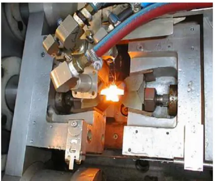
Four filler wires and a conventional experimental wire were chosen and bead-on-plate welds were initially deposited on four plates of different thickness using Gas Metal Arc Welding process (GMAW). Distortion measurements were conducted in order to compare the distortion behavior among all the wires. These measurements were compared with the calculated values using the numerical modeling software Sysweld. Residual stresses were also calculated using the software and all the results were compared for all the different wires. Metallographic samples were prepared and etched to reveal the macro and microstructures. Carbon equivalent values were calculated by changing the compositions of chromium, nickel and carbon. The change in alloy hardenability is expressed by carbon equivalent. Composition was analyzed to investigate which element caused the metal to distort and the effect that it had on martensite start temperature. Abinit and VASP software were used to calculate, albeit in a preliminary fashion, lattice properties of iron, nickel and chromium alloys. Also, Huey test or the nitric acid test was conducted on the LTTW alloys to measure the susceptibility of the LTTW to intergranular attack.
1.3 Organization of the Thesis
The layout of this thesis consists of seven subsequent chapters. Chapter One provides an introduction which includes the preface of the research topic. This chapter also gives the justification for carrying out this work and puts forth the objectives of the conducted study. This chapter also summarizes the experimental work conducted.
7
Chapter Two discusses the background literature on LTTW consumables and the research accomplishments in the recent past. It also demonstrates gaps in the knowledge base that provides the basis for the development of this work.
Chapter Three concentrates on the calculations and theoretical approach that was conducted in this work related to martensite start temperatures. It defines the basis upon which the experimental wires were selected. It gives a brief introduction to how Sysweld works in modeling stresses and distortion. It presents a short overview to ABINIT-VASP that was used to calculate selected lattice properties for Fe-Ni-Cr atoms arrangements. Finally some calculations of carbon equivalent values were conducted based on the compositions to investigate the affects of alloying elements on crystal properties.
Chapter Four covers the experimental procedure that was adopted to measure out-of-plane distortion on bead-on-plate welds by using LTTW wires and the conventional experimental wire. It also gives a procedure of the Huey test that was carried out to observe the corrosion behavior of the welds.
Chapter Five discusses the welding simulation analysis, which explains the thermal history of the wires and the base metal. It also shows the effects of the different experimental LTTW wires on distortion and residual stress.
Chapter Six describes the results and discussions that were obtained from the experiments. It also compares the measurements obtained both experimentally and theoretically.
Chapter Seven presents conclusions that summarize the main findings of the research conducted, the major results drawn from the observations and also suggests a direction and topics for future work in this area of research.
8 Chapter 2
Literature Review
This chapter provides relevant information for the reader to understand and interpret the data in the subsequent chapters. This chapter explains the importance of using Low Transformation Temperature Welding consumables to develop compressive residual stresses in welded joints by inducing martensite transformation.
2.1 Residual Stress and Distortion Management in Welded Joints
The problem of predicting residual stresses due to welding has long been recognized by structural designers and fabricators as very important but difficult. During welding the metal is melted by the application of extreme heat. After completion of solidification and after cooling there generally is a tensile residual stress established in the vicinity of the weld joint which gives rise to distortion. This stress is caused by the dissimilar volumetric contraction around the weld due to slight differences in the thermal history. These stresses predominantly occur in the weld toe region and are deleterious since they reduce the fatigue life of the weld component. Corrosion cracking and brittle fracture may also occur. In order to remove the tensile residual stresses methods like shot peening and post weld heat treatment are typically used [7, 8, 9].
Shot peening is an effective method of improving the fatigue strength of components and structures. Multiple effects are induced by shot peening. Plastic deformation induces a residual compressive stress in a peened surface, along with tensile stress in the interior. Surface compressive stresses confer resistance to metal fatigue and to some forms of stress corrosion. The tensile stresses deep in the part are not as problematic as tensile stresses on the surface because cracks are less likely to start in the interior. In most shot peening applications, uniform
9
residual compressive stress in the surface zone is the desired effect. These compressive stresses will resist the formation of fatigue cracks within the component during service, thereby improving significantly the life of the peened component [10, 11,12].
Post weld heat treatment (PWHT) is commonly used to reduce tensile residual stresses. Post Weld Heat Treatment is a heating and cooling treatment given to a weldment in order to relieve the tensile residual stresses. Care should be taken to maintain the temperature at a normal range. Higher temperature leads to faster increase in temperature in thin sections than the thick sections. Similar condition also appears when the temperature is low, that is, the temperature decreases fast in the thin sections than the thick sections. Residual stresses, distortion, cracks and fracture can result from non uniform heating and cooling [13].
Flame straightening is one of the methods used to control distortion. But it leads to additional costs towards labor, materials and process time.
Unfortunately all these methods have their drawbacks and are not efficient in reducing or diminishing the deleterious tensile residual stresses [14].
2.2 Carbon Equivalent Concept
Carbon Equivalent (CE) is an empirical value in weight percent, that relates the combined effects of different alloying elements used in the making of carbon steels to an equivalent amount of carbon to express hardenability and cracking susceptibility. By varying the amounts of carbon and other alloying elements in the steel, the desired strength levels can be achieved by proper heat treatment. A better weldability can also be obtained. Carbon equivalent is a rating of weldability related to C, Mn, Cr, Mo, V, Ni and Cu content. There are several commonly used equations for expressing Carbon Equivalent, each with different coefficients assigned for the
10
alloying elements. The most important of all the CE equations is the International Institute of Welding (IIW) carbon equivalent equation which is:
CE = C + (Mn/6) + (Ni/15) + (Cu/15) + (Cr/5) + (Mo/5) + (V/5)
The concentration of the alloying elements is given in weight percent. It can be seen in the above equation that carbon is the element that most affects weldability. Together with other chemical elements, carbon may affect the solidification temperature range, hardenability and cold-cracking behavior of a steel weldment. Figure 2.1 below summarizes the CE and weldability description of some steel families. Steels with low CE are generally weldable while high CE steels are more difficult to weld. The application of CE expressions is empirical [15].
11
Several expressions are also available for other steel groups with a wider range of alloying elements and with different prior heat treatments, hydrogen contents and weld hardness. [15] Another CE type equation is:
PH = Pcm + 0.075 log10 H + (Rf/40)
Where, PH is the cracking susceptibility parameter, H is the concentration of hydrogen (
ppm), Rf is the restraint stress (MPa). Pcm in this equation is calculated using the Ito-Bessyo equation, developed in the 1970’s for microalloyed steels.
Pcm = C + (Mn/20) + (Si/30) + (Cu/20) + (Ni/60) + (Cr/20) + (Mo/15) + (V/10) + 5B
The Pcm equation can be used independently to indicate the weldability of microalloyed steels as well.
2.3 The Martensitic Transformation in Steels
Martensite in steel is a product of the rapid, diffusionless transformation of austenite. Martensite in steels is a metastable body-centered tetragonal (BCT) phase of iron containing carbon. For martensite to form, a rapid cooling of the parent phase is required, so that carbon and other solute atoms cannot partition into other nucleation and growth products like α-ferrite and cementite (Fe3C). This rapid cooling will cause the solubility of interstitial atoms like carbon to
be greatly exceeded, turning the phase to be metastable. If martensite is heated to a temperature where the carbon mobility is enhanced, this element will diffuse to form carbides, while decomposing the supersaturated martensite to equilibrium ferrite [5, 16].
The formation of martensite is influenced by two different sets of factors: 1) those that alter the equilibrium temperature (To) between martensite and austenite, and 2) those that affect
12
the required undercooling (ΔTm =To-Ms) for the martensitic reaction to occur. Diffusion, nucleation and growth are not involved in the transformation of austenite to martensite. Martensite can form at very low temperatures, where diffusion of atoms, even of interstitials, is not conceivable. As such, martensite has exactly the same composition as the parent austenite does [17]. The austenite decomposition occurs when the temperature is lowered sufficiently to activate the martensite nuclei. This phase formation occurs in such a short time that no classic nucleation and growth process could be applicable. Proof of this activation manner is the fact that martensite can nucleate at temperatures close to the absolute zero, where the thermal vibration is so small that it could not be capable of triggering any process. Another reason for the non equilibrium state is that the shape deformation associated with martensitic transformation causes strains and that the resulting strain energy must be accounted before the transformation can occur. The carbon atoms partition between cementite and ferrite is suppressed as a result of rapid cooling. They are trapped in the octahedral sites of a body-centered cubic (BCC) producing new phase structure. At low temperature, the FCC phase cannot transform into the stable BCC phase because carbon atoms mechanically hinder the rearrangement of the iron into a BCC crystal [18].
The body centered tetragonal structure of martensite is similar to that of iron which is a BCC crustal; however the carbon atoms are all placed randomly in the interstitial sites, 0,1/2,1/2 sites, which results in lengthening of the c-axis. A good crystallographic coupling is emphasized between the parent and product phases. The martensite habit plane is very close to {225} plane in the austenite. There are twelve {225} planes and two possible twin-related orientations the slip and mechanical twinning of the martensite for each habit plane. Therefore, there are 24 possible orientation relationships between the lattices in the martensite and in the austenite of the steel. It
13
states that the {101} planes of martensite are parallel to the {111} plane of the parent austenite. At the same time, the {111} direction in the martensite is parallel to the {110} direction of the austenite. The Bain distortion which is explained earlier in the introduction causes a rotation away from the habit plane and a number of the cells of the parent phase will transform to new lattice. The martensite will then deform within the original boundary with a lattice invariant deformation. In this case the martensite will deform by slip or by twinning [19].
Two different temperatures define the martensitic transformation: Ms and Mf. The martensite start transformation temperature (Ms) is the temperature at which austenite starts transforming into martensite. The transformation from austenite to martensite proceeds as the temperature is reduced below Ms until the martensite finish temperature (Mf) is reached, at which point 100% martensite is expected [20].
2.4 Transformation-Induced Compressive Residual Stresses
After welding, the molten metal and the adjacent region of the weld cools down, the metal shrinks due to the reduction in vibrational amplitude of their atoms. After complete solidification and further cooling, a tensile residual stress develops between the weld and the base metal. The smaller the arc distance and higher the temperature, the greater the material shrinks, and the higher are the final residual stresses. The presence of the tensile residual stresses in a weldment dramatically reduces the fatigue limit of the joint. Many researchers have studied the effects of these harmful residual stresses on the fatigue strength of weldment and concluded that the fatigue life of a component increases when a compressive residual stress is present, especially on the surface [21, 22].
14
Previous literature reports that a Low Transformation Temperature Welding (LTTW) wire that contained 10 wt. pct. chromium and 10 wt. pct. nickel was developed for the gas metal arc welding process. This consumable was capable of developing residual stresses by martensitic transformation and with expansion of the weld metal near room temperature. The authors also verified that the fatigue strength of the welded joints made using the LTTW wire was improved without post-heating treatment [23]. Figure 2.1 shows the conventional welding with expansion beginning around 600ºC and continuing till 500ºC due to austenite decomposition. After the finish of the transformation, the weld shrinks again. At these high temperatures austenite typically decomposes into ferrite and carbides. However, the developed solid wire (10 wt. pct. Cr and 10 wt. pct. Ni) shows that the martensitic transformation starts around 280ºC, with expansion peaking around 100ºC to ambient temperature. As no further thermal contraction occurs, the expansion due to martensitic transformation and its effects remain [24, 25].
The tensile residual stresses are due to the shrinkage that occurs in the weld metal in the case of the conventional welding consumable and the compressive residual stresses are due to the expansion that occurs in the deposit using low transformation temperature welding consumable as shown in Figure 2.2.
Figure 2.2: (a) Relationship between strain and temperature during cooling; (b) Development of stress during cooling.
15
This compressive residual stress brought about by the low transformation temperature welding consumable improves the fatigue life of the material. The fatigue limits of the welds deposited by the LTTW consumables were three time higher than that of the conventional wire as shown in the Figure 2.3[26, 27, 28].
Figure 2.3: Comparison of the conventional and the developed wire in terms of fatigue life
2.5 Relationship between Residual Stresses and Distortion
Two of the major problems of any fusion welding process are residual stress and distortion. Residual stress is primarily caused by the compressive yielding that occurs around the molten zone as the material heats and expands during welding. When the weld metal cools it contracts which causes a tensile residual stress, particularly in the longitudinal direction. After welding a residual tensile stress remains across the weld centerline and causes a balancing compressive stress further from the weld zone. The tensile residual stress on the weld line reduces the fatigue strength and the toughness, particularly when combined with any defects associated with the
16
weld bead. To relieve some of the residual stresses caused by the welding process, the structure deforms, causing distortion. In conclusion, greater the compressive residual stress, lesser is the expected distortion [30,3].
2.6 Alloying Elements and Elastic Property – Bulk Modulus
Most metals are not used in their pure form but have alloying elements added to them to change their properties.
Manganese
All commercial steels contain 0.3 to 0.8 wt. pct. manganese, for deoxidation and strengthening purposes. Any manganese in excess of deoxidation requirements partially dissolves in the iron and partly forms Mn3C. There is a tendency nowadays to increase the manganese
content and reduce the carbon content in order to get steel with an equal tensile strength but improved ductility [31].
If the manganese is increased above 1.8 wt. pct. the steel tends to become air hardened, with resultant impairing of the ductility. The manganese content is also increased in certain alloy steels, with a reduction or elimination of expensive nickel, in order to reduce costs. Steels with 0.3-0.4 wt. pct. carbon, 1.3-1.6 wt. pct. manganese and 0.3 wt. pct. molybdenum have replaced 3% nickel steel for some purposes.
Non-shrinking tool steels contain up to 2 wt. pct. manganese, with 0.8-0.9 wt. pct. carbon. Steels with 5 to 12 wt. pct. manganese are martensitic after slow cooling and have little commercial importance. Manganese steels contain 12 to 14 wt. pct. of manganese and 1.0 wt. pct. of carbon. These steels are characterized by a great resistance to wear and are therefore used for
17
railway points, rock drills and stone crushers. Annealing embrittles the steel by the formation of carbides at the grain boundaries. Nickel is added to electrodes for welding manganese steel and 2% Mo sometimes added, with a prior carbide dispersion treatment at 600°C, to minimize initial distortion and spreading.
Nickel
Nickel and manganese are similar in behavior and both lower the eutectoid temperature. This eutectoid decomposition temperature upon heating is lowered progressively with increase of nickel (approximately 10°C for 1% of nickel), but the lowering of eutectoid on cooling is greater and irregular. The addition of nickel acts similarly to increasing the rate of temperature cooling of carbon steel.
Steels with 0.5 wt. pct. nickel are similar to carbon steel, but are stronger, on account of the finer pearlite formed and the presence of nickel in solution in the ferrite. When exceeding 10 wt. pct. nickel the steels have a high tensile strength, great hardness, but are brittle. When the nickel is sufficient to produce austenite the steels become non-magnetic, ductile, tough and workable, with a drop in strength and elastic limit.
Carbon intensifies the action of nickel. Steels containing 2 to 5 wt. pct. nickel and about 0.1 wt. pct. carbon are used for case hardening; those containing 0.25 to 0.40 wt. pct. carbon are used for crankshafts, axles and connecting rods.
The superior properties of low nickel steels are best brought out by quenching and tempering (550-650°C). Martensitic nickel steels are not utilized and the austenitic alloys cannot compete with similar manganese steels owing to the higher cost.
18 Chromium
Chromium can dissolve in either alpha- or gamma-iron, but, in the presence of carbon, carbides such as cementite (Fe,Cr)3C in which chromium may rise to more than 15% are formed.
Chromium carbides such as (Cr,Fe)3C2, (Cr,Fe)7C3, (Cr,Fe)4C can also be formed. Stainless steels
typically contain Cr4C. The pearlitic chromium steels with, say, 2% chromium are extremely
sensitive to rate of cooling and temperature of heating before quenching.
When chromium exceeds 1.1 wt. pct. in low-carbon steels an inert passive film is formed on the surface which resists attack by oxidizing reagents. Still higher chromium contents are found in heat-resisting steel.
Chromium steels are easier to machine than nickel steels of similar tensile strength. The steels of higher chromium contents are susceptible to temper brittleness if slowly cooled from the tempering temperature through the range of 550 to 450°C. These steels are also liable to form surface markings, generally referred to as "chrome lines".
The chromium steels are used wherever extreme hardness is required, such as in dies, ball bearings, plates for safes, rolls, files and tools. High chromium content is also found in certain permanent magnets.
Nickel and chromium
Nickel steels are noted for their strength, ductility and toughness, while chromium steels are characterized by their hardness and resistance to wear. The combination of nickel and chromium produces steels that exhibit all these properties, some intensified, without the disadvantages associated with the simple alloys. The depth of hardening is increased, and with 4.5 wt. pct.
19
nickel, 1.25 wt. pct. chromium and 0.35 wt. pct. carbon the steel can be hardened simply by cooling in air.
Low nickel-chromium steels with small carbon content are used for case hardening, while for most constructional purposes the carbon content is 0.25-0.35%, and the steels are heat-treated to give the desired properties. Considerable amounts of nickel and chromium are used in steels for resisting corrosion and oxidation at elevated temperatures.
Molybdenum
Molybdenum dissolves in both alpha- and gamma-iron and in the presence of carbon forms complex carbides (Fe,Mo)6C, Fe21Mo2C6 and Mo2C.
Molybdenum up to 0.5% appears to be more effective in retarding pearlite and increasing bainite formation. Additions of 0.5 wt. pct. molybdenum have been made to plain carbon steels to give increased strength at boiler temperatures of 400°C, but the element is mainly used in combination with other alloying elements.
Ni-Cr-Mo steels are widely used for ordnance, turbine rotors and other large articles, since molybdenum tends to minimize temper brittleness. Molybdenum is also a constituent in some high-speed steels, magnet alloys, heat-resisting and corrosion-resisting steels.
Tungsten
Tungsten dissolves in gamma-iron and in alpha-iron. With carbon it forms WC and W2C,
but in the presence of iron it forms Fe3W3C or Fe4W2C. A compound with iron-Fe3W2-provides
an age-hardening system. Tungsten raises the critical points in steel and the carbides dissolve slowly over a range of temperature. When completely dissolved, the tungsten renders
20
transformation sluggish, especially to tempering, and use is made of this element in most hot-working tool (“high speed”) and dies steels. Tungsten refines the grain size and produces less tendency to decarburization during working. Tungsten is also used in magnet, corrosion and heat-resisting steels.
Silicon
Silicon dissolves in the ferrite, of which it is a fairly effective hardener, and raises the Ac and the Ar temperatures when slowly cooled and also reduces the gamma-alpha volume change. Only three types of silicon steels as shown in Table 2.1 are in common use - one in conjunction with manganese for springs; the second for electrical purposes, used in sheet form for the construction of transformer cores, and poles of dynamos and motors, that demand high magnetic permeability and electrical resistance; and the third is used for automobile valves.
Table 2.1 : Three types of Silicon Steel
C Si Mn
1. Silico-manganese 0.5 1.5 0.8
2. Silicon steel 0.07 4.3 0.09
3. Silichrome 0.4 3.5 8
Silicon contributes oxidation resistance in heat-resisting steels and is a general purpose deoxidizer.
21
Copper dissolves in the ferrite to a limited extent; not more than 3.5 wt. pct. at normalizing temperatures, while at room temperature the ferrite is saturated at 0.35 wt. pct. It lowers the critical points, but insufficiently to produce martensite by air cooling. The resistance to atmospheric corrosion is improved and copper steels can be temper hardened.
Cobalt has a high solubility in alpha- and gamma-iron but a weak carbide-forming tendency. It decreases hardenability but sustains hardness during tempering. It is used in "Stellite" type alloys, gas turbine steel, magnets and as a bond in hard metal.
Bulk Modulus
It is a numerical constant that describes the elastic properties of a solid or fluid when it is under pressure on all surfaces. The applied pressure reduces the volume of a material, which returns to its original volume when the pressure is removed. Sometimes referred to as the incompressibility, the bulk modulus is a measure of the ability of a substance to withstand changes in volume when under compression on all sides. It is equal to the quotient of the applied pressure divided by the relative deformation.
In this case, the relative deformation, commonly called strain, is the change in volume divided by the original volume. Thus if the original volume Vo of a material is reduced by an applied pressure p to a new volume Vn, the strain may be expressed as the change in volume, Vo – Vn, divided by the original volume, or (Vo-Vn)/Vo. The bulk modulus, by definition, is the pressure divided by the strain, may be expressed mathematically as
Bulk Modulus = Pressure/ Strain =
22 Hooke’s law of elasticity.
2.7 Low Transformation Temperature Consumables Concept
Various equations were selected in order to calculate Ms and Mf temperatures as they both are important parameters in structural steel welding because of their influences on residual stress development in the weld [32]. There were many formulas developed through the years to relate martensitic transformation temperatures to steel chemical composition as illustrated below:
2.7.1 Martensitic Start Temperature Equations:
Ms is denoted as Martensite start temperature.
2.7.1.1 Payson & Savage:
Ms (ºF) = 930- 570C – 60Mn – 50Cr – 30Ni – 20Si – 20Mo – 20W
The Payson & Savage equation is applicable for alloy steels that contain up to 0.5 wt. pct. carbon content. It is also assumed that austenitizing temperature is one at which all the carbides will be completely in solution in the austenite. In the Payson and Savage equation, carbon has by far the greatest effect in depressing the Ms point. This equation was developed based on microstructural analysis in determining the Ms temperatures.
2.7.1.2 Carapella
Ms (ºF) = 925(1-0.620C)*(1-0.092Mn)*(1-0.033Si)*(1-0.045Ni)*(1-0.070Cr)*(1-0.029Mo)*(1-0.081W)*(1+0.120Co)
Unlike the Payson and Savage equation, Carapella’s equation has a multiplicative form rather than the additive form. Again, the metallographic technique was used in the identification
23
of the transformation start temperatures in the Carapella equation.
2.7.1.3 Rowland & Lyle
Ms(ºF) = 930 – 600C – 60Mn- 50Cr – 30Ni-20Si -20Mo-20W
Rowland and Lyle suggested that the carbon factor proposed by Payson and Savage should be raised from 570 to 600. Rowland studied carbon steel materials with the Carbon content ranging between 0.4 to 1.0 wt. pct. However, they were unable to obtain adequate agreement between their experimental observation and the calculated values.
2.7.1.4 Nehrenberg
Ms(ºF) = 930 – 540C – 60Mn – 40Cr -30Ni -20Si- 20Mo
Since there was a lack of agreement between the calculated and experimental values, Nehrenberg reviewed all the data and obtained an equation based on the experimental work of Payson and Savage. Nehrenberg used lower factors for carbon and chromium resulting in increasing the composition required for the same Ms point.
2.7.1.5 Grange & Stewart
Ms(ºF) = 1000 – 650C – 70Mn – 70Cr – 35Ni – 50Mo
Grange and Stewart used metallographic analysis where the percentage of martensite observed is plotted against the quenching temperature for carbon and low alloy steels. This equation is fairly good at estimating Ms temperatures for low alloy steels. The success of the microscopic method for the determination of the temperature range within which martensite forms will depend on the accurate observation.
24 2.7.1.6 Steven and Haynes
Ms(ºC) = 561 – 474C – 33Mn – 17Cr – 17Ni – 21Mo
Steven and Haynes studied the martensitic transformation behaviors of a wide variety of steel compositions and established a new empirical equation that related alloy composition and transformation temperature. In this work, microscopic method, X-ray diffraction, and dilatometric analysis were carried out to experimentally identify the Ms temperatures. Adequate agreement was observed between the experimental and the calculated values. Their study was conducted on carbon and low alloy steels such that the equation may not be appropriate to be used in the current research.
2.7.1.7 Andrews (Linear)
Ms(ºC) = 539 – 423C – 30.4Mn – 12.1Cr – 17.7Ni – 7.5Mo
Andrew obtained later empirically, from 184 different steels, linear and non linear equations for the calculation of Ms temperature. The linear equation can be applied generally within the composition limits (0.1 to 0.6 wt. pct. C, 0.04 to 4.9 wt. pct. Mn, Ni < 5.0 wt. pct., Cr < 4.6 wt. pct., Mo < 5.4 wt. pct.).
2.7.1.8 Andrews (Product)
Ms (ºC) = 512 – 453C + 15Cr – 16.9Ni – 9.5Mo + 217C2 – 71.5C*Mn – 67.6C*Cr
Andrew’s preliminary analysis indicated strong significance for the C2 term which had approximately half the co-efficient of C with opposite sign. In general, the linear formula is adequate but the non linear formula involving product and C2 terms is likely to be more accurate
25 for higher contents of alloying elements.
2.7.1.8 Eichelmann and Hull
Ms(ºC) = 1305 – 41.7Cr – 61.1Ni – 33.3Mn – 27.8Si – 1667(C+N)
Eichelmann and Hull equation does not include the effect of Mo in determining the Ms temperature.
2.7.1.9 Monkman
Ms(ºC) = 1182 – 36.7Cr – 56.7Ni – 1456(C+N)
Monkman found that the influence of C and N is not linear.
2.7.1.10 Self & Olson
Ms(ºC) = 521 – 14.3Cr – 17.5Ni – 2809Mn – 37.6Si- 350C – 29.5Mo + 23.1(Cr + Mo)*C – 1.19*Cr*Ni
Self and Olson used more parameters in the equation including some cross-product terms of alloying elements. The effect of carbon on the Ms temperature was considered. Since the Self and Olson equation was derived statistically based on a number of alloys, this equation is expected to provide accurate results for alloys whose compositions are within the range of the database.
2.7.1.11 Ghosh and Olson
Ghosh and Olson proposed a model to describe the composition dependency of the critical driving force for martensitic formation, including the effect of both interstitial and substitutional solutes. Ghosh and Olson provided the parameters for a number of elements (C, N, Mn, Si, Cr, Nb, V, Ti, Mo, Cu, W, Al, Ni, Co). The ΔGγ-M can be used to calculate the Ms temperature
26 using the Kaufmann equation below.
ΔGγ-M
= 526 – 42Ms
Developed Wires:
Earlier work at CSM developed four LTTW electrodes A1, A6, B5 and C5 based on the original 10 wt. pct. Cr and 10 wt. pct. Nickel composition to produce ferrite – martensite and ferrite – austenite microstructure. These wires were developed to investigate the Ms temperature of the welds and the effect of transformation temperatures on microstructural development. The sizeable matrix of welding alloys was calculated using the Ms equations discussed in the previous paragraphs spanned across the entire martensite field on the Schaeffler constitution diagram as shown in Figure 2.4. The Schaeffler diagram gives a quantitative description of the ferrite content and the lines are linear. The diagram provides the correlation of the effect of the austenite stabilizers and ferrite formers on the microstructure of the weld metal. Ferrite stabilizers are alloying elements that tend to promote the formation of BCC α phase. The austenite stabilizers are the alloying elements that tend to promote the FCC γ phase. Chromium and Nickel contents were set not to exceed ten wt. pct. since previous studies presented the 10 wt. pct. Chromium and 10 wt. pct. Nickel as the most appropriate combination to produce martensitic transformation – induced compressive residual stresses in the weld metal limiting the amounts of Cr and Ni also helps to lower the cost of the experimental consumables. The Creq and Nieq on the Schaeffler diagram can be calculated using the two equations that follow.
Creq = Cr + Mo + 1.5*Si + 0.5*Nb
27
Figure 2.4: Part of the Schaeffler constitution diagram representing the distribution of the a lloys investigated
It is interesting to note that alloys with very different Nieq and Creq were found to exhibit similar Ms temperature. Naturally, questions related to the effect of alloying elements on austenite – martensitic transformation must be raised. For example, is Ms a good indicator to describe the LTTW behavior. The Ms equations used in the research work were Self and Olson, Eichelmann and Hull, Ghosh and Olson equations. These equations have been developed for
28
stainless steels and high alloys which make them more appropriate to be used for the range of chromium – nickel alloy compositions in this work.
Ms temperatures were calculated for four sets of different chemical compositions which were identified on the isotherm lines contour mappings as shown in the Figure 2.5. The first two sets of chemical compositions have been selected specifically along 200 ºC and 350 ºC, respectively, using the Self and Olson formula. Using the Ghosh and Olson equation the Ms temperatures were calculated for the materials selected. This equation shows the martensite start temperatures of 163 ºC, 219 ºC, 157 ºC and 177 ºC for the SO200A, SO200B, SO350A and SO350B welding wires as shown in the Table 2.2. Once the Ms values were calculated, experimental analysis using dilatometric test were conducted to reveal which of the models better evaluated the Ms transformation temperatures.
Figure 2.5: Contour mapping for isotherm martensitic transformation temperature versus Creq
29
Table 2.2: Ms Temperatures calculated for the set of welding consumables as shown on the Self and Olson contour mapping
Method
Martensitic Transformation Start Temperature (Ms) in C
SO-200A SO-200B SO-350A SO-350B
Ghosh and Olson (1994) 163 219 157 177
Eichelmann and Hull (1953) 446 528 935 985
Self and Olson (1986) 200 200 350 350
Dilatometric measurements were conducted on a Gleeble 1500 thermo-mechanical simulation system to experimentally measure the Ms temperature as shown in the Figure 2.6. This figure shows a general view of the test chamber and the details of a typical sample set up for dilatometry work. A solid cylindrical sample of 6.0 mm diameter and 80 mm length was extracted from a multipass weld as shown in the Figure 2.7. This weld metal was subjected to thermal cycles to mimic the cooling behavior that austenite in steels undergoes after welding. The sample temperature was measured by thermocouples welded to its middle surface circumference. The sample was austenitized at 1100 ºC for eight seconds followed by cooling at a constant rate of 30 ºC/s to ambient temperature. The heating rate was 80 ºC/s. This Gleeble test was carried out for all the samples welded with these wires. The main objective of conducting this test is to determine the Ms temperature and Expansion point. The Gleeble test was conducted for all the samples welded using SO200A, SO200B, SO350A and SO350B. The test was carried using different cooling rates. The graph goes from the positive axes to the negative axes where the positive axes as the tensile residual stress and the negative axes is treated as the compressive residual stress. This means the samples goes from contraction to expansion when it reaches the Ms temperature.
30
Figure 2.6: View of the Gleeble 1500 testing chamber
Figure 2.7: A schematic drawing showing the location in the multipass weld feed from which the sample was extracted for a cylindrical dilatometric sample(in mm)
Ms is identified as the temperature at which the slope changes from positive to negative during cooling. The dilatometry test results are plotted in all the four designed welding wires as
31
shown in Figure 2.8. Sample SO200B exhibited the lowest Ms temperatures and the largest amount of expansion (+27 μm). The other samples made by the welding wires, SO200A, SO350A and SO350B, revealed expansive elongations of +20 μm, +13 μm and +5μm, respectively.
Figure 2.8: Dilatometric curves of the welds made by the developed wires indicating Ms temperature with CR of 30 ºC/s., a) the dilatometric curve for SO200A b) the dilatometric curve for SO200A c) the dilatometric curve for SO200A d) the dilatometric curve for SO200A
32
Data from Alghamdi in Table 2.3 shows the experimentally determined Ms temperatures values compared with the estimated values using Self and Olson (SO) and Eichelmann and Hull (EH) equations as well as the Ghosh and Olson (GO) methodology. Self and Olson equation appeared to better predict the Ms temperatures for the experimental alloys than EH and GO equations. Ms temperatures for the alloys used in this work were calculated using only the Self and Olson and Eichelmann and Hull equations.
Table 2.3: Experimental Ms temperatures compared with the predicted calculations
Welding Wire
Self and Olson
Ghosh and Olson Eichelmann and Hull
Experimental Ms temperature (°C) SO-200A 200 163 446 160 SO-200B 200 219 528 190 SO-350A 350 157 935 375 SO-350B 350 177 985 410
Distortion was determined for the welds deposited on a ½ in. thick plate using wires developed by the calculation after the Self and Olson equation. The results were plotted in terms of distortion angles as shown in Figure 2.9. The graph shows that SO200B produced lowest distortion. The distortion angles observed in these welds were calculated using the equation:
33
where, X = H – W, where H is the total height from the top surface of the work piece to the flat ground surface, W is the thickness of the welded work piece and Y is the distance from the edge of the welded plate to the centerline of the weld.
Figure 2.9: Different transverse deformation produced by various LTT welding consumables and the commercial welding wire
2.8 Density Functional Theory (DFT)
Apart from the martensite start temperatures, changes in alloying composition also play a very important role in inducing compressive residual stresses and decreasing distortion. The wires with higher chromium were observed to behave in a different fashion when compared to the wires with higher nickel. As a result of which Quantum Mechanic calculations were used to
0.00 0.50 1.00 1.50 2.00 2.50 3.00 3.50
SO200A SO200B SO350A SO350B ER70S-3
T rans v ers e D is tort ion Angle
34
calculate the bulk modulus of the alloying elements. The Density Functional theory (DFT) is presently the most successful approach to compute the electronic structure of matter. Its applicability ranges from atoms, molecules and solids to nuclei and quantum and classical fluids. The DFT provides the ground state properties of a system, and the electron density plays a key role. DFT predicts a great variety of molecular properties: molecular structures, vibrational frequencies, atomization energies, ionization energies, electric and magnetic properties, reaction paths etc. The DFT has been generalized to deal with many different situations: spin polarized systems, multicomponent systems such as nuclei and electron hole droplets, free energy at finite temperatures, superconductors with electronic pairing mechanisms, relativistic electrons, time-dependent phenomena and excited states, molecular dynamics, etc. The calculations of DFT are simple to implement yet often very accurate. The relatively low cost makes the DFT at present the only choice for calculations for systems with large number of electrons. DFT uses Ab initio nuclear structure calculation primarily based on approximating the many-nucleon wave function. DFT derives its basics from the Hohenberg-Kohn theorem. In short the Hohenberg–Kohn theorem demonstrates that the ground state properties of a many-electron system are uniquely determined by an electron density that depends on only 3 spatial coordinates. It lays the groundwork for reducing the many-body problem of N electrons with 3N spatial coordinates to 3 spatial coordinates, through the use of functionals of the electron density. This theorem can be extended to the time-dependent domain to develop time–dependent density functional theory which is used to describe excited states. [33] In this work preliminary calculations using Ab initio modeling have been conducted and summarized in the Results and Discussion section.