Soil Analysis for samples from the hill-fort of Hedeby

(1)

Soil Analysis for samples from the

hill-fort of Hedeby

Kandidatuppsats i laborativ arkeologi Stockholms Universitet

HT 2014 Fig. 1: Trench 2012 showing layer 14 where the scale is positioned. Photo toward the south. (Kalmring, In press).

(2)

Abstract

Hedeby Hochburg, borgen i Hedeby, har fått förhållandevis lite uppmärksamhet, jämfört med själva samhället i Hedeby. Utgrävningen från 2012 har dock väckt ett intresse, med ett antal frågor som behöver besvaras. I denna uppsats analyseras jordprover som samlats under utgrävningen, för att se om de kan visa något om den kronologiska relationen mellan borgvallen och gravarna i borgen. Tre metoder användes, FTIR (Fourier Transform Infrared Spectroscopy), röntgendiffraktion och röntgenfluorescens. Resultaten från XRF och XRD

visar på en rumslig relation mellan minst en av vallens konstruktionsfaser och nedsänkningen i

ett lager innanför vallen. Relationen med gravarna är inte tydlig än, och analysen gav inga

kronologiska ledtrådar. Resultatet kan användas som hypotes för vidare prövning i framtiden.

2

4

6 3.2

(3)

1. Introduction

Archaeology is a dynamic, interdisciplinary field that is evolving constantly as archaeologists are developing traditional analysis methods; dropping the out-dated, less reliable ones; and incorporating newer methods adapted from other branches of science when they prove to be effective in answering questions related to the archaeological narration.

Soil and sediment analysis techniques are at the centre of this evolution, contributing to the development of important aspects of archaeological research. Humans leave variety of morphological traces to their existence, whether on the “macro-scale” or on the “micro-scale” (Moore et al. 1988; Hjulström et al. 2009) . These analysis techniques could be used to trace humans; as it has been proved useful in different stages within the archaeological work, from early stages of site prospection, well into the interpretation phase (Wilson et al. 2008). Thus, systematically integrating soil analysis in the archaeological work is logical and beneficial on several levels, from providing more reliable data for interpretation to reducing costs on the longer term. It is also an almost constantly attainable procedure because it's hard to imagine a site lacking soil or sediment material that could be analysed in some way to gain more knowledge about it.

Chemical soil analysis methods covers a wide range from the traditional “wet chemistry” methods, like element extraction by acids, to instrumental methods for specific tests, like emission spectroscopy or absorption spectroscopy. However, the degree to which each of these methods will result in effective archaeological data for a given case depends hugely on site-specific circumstances, research aim, question formulation, process planning, and the actual process of collecting and treating the samples. These analytical chemistry methods are also used in other fields of research, like environmental studies, soil science, geomorphology, and quaternary geology (Ohse et al. 1984), to name some.

Soil analysis in archaeology had its pioneers identifying anthropogenic influences when Arrhenius found in the 1930s a clear connection between phosphate enrichment and prehistoric sites. Much development has happened since then and other elements were added as a human occupancy markers while taking into account the natural variations in the existence of these elements (Linderholm et al. 1994) .

The process of tracing humans via soil analysis has to deal with more than the anthropogenic alteration of a number of elements; certain considerations of natural processes has to be dealt with, as many other factors affect those elements like parent material,

(4)

biological influences, and pedogenic processes. Moore and Denton (1988) Sampled areas unaffected by humans when making their study on sites in Northern Quebec for comparison. They emphasized on the importance of being cautious when trying the understand the extent of anthropogenic influences and contrasted Ca to P as being much less reliable. These ideas were further developed and integrated into the methodology used for the analysis, specially in regard to what “natural” levels are.

Another step forward in the field was combining inorganic and organic chemical analysis to produce reliable results when trying to identify activity areas within a site (Hjulström et al. 2009) . The same paper by Hjulström and Isaksson (2009) discussed the very important question mentioned above of whether establishing a natural background to compare anthropogenically affected areas to is a viable approach. It came to the result that establishing a background is not possible if a matching, yet “untouched” source material isn't identified off-site, since any comparison with a background would be unreliable because of natural variations occurring sometimes at a very small spatial scales.

Like any other archaeological question, there is no one ready-made solution to apply automatically to get the desired result. The case of the rampart at the hill-fort of Hedeby discussed in the paper does not demand an in-depth approach in analysing the soil samples. Hence, organic chemical analysis and trace element analysis would be unnecessary because of the nature of the site and the questions which should be answered at this stage. More details about the adapted approach is in the Purpose and aim section.

2. Hedeby

4 Fig. 2: Danevirke's location in Schleswig-Holstein marked in white rectangle in the first map to the left. Its location in relation to Hedeby in the upper map to the right. And lastly, the rampart of Hedeby in relation to the hill-fort of Hedeby (white polygon) in the lower map to the right. Maps are from Open Street Maps, processed in ArcGIS 10.1.

(5)

The hill-fort of Hedeby, the Hochburg, lays north-east of the Viking settlement of Hedeby on a ridge plateau, by the lake Haddebyer Noor, nowadays in the north of Germany. Not a lot is known of the hill-fort, despite its spatial closeness to the well-studied settlement, maybe even because of this closeness (Kalmring In press), the story of this site has been historically obscured since the attention was naturally turn to the main Viking settlement. Still, addressing the hill-fort archaeologically has to take into attention this proximity to the settlement.

The first time the site’s semi-circular rampart of the settlement was identified as the same Hedeby mentioned in the rune stones from the same area was 1898 by a Danish archaeologist called Müller. The earliest building phase of the semicircular rampart around the settlement of

Hedeby was dated to around the 10th _{century CE (Dobat 2008, 39). Also, since the}

semicircular wall around the settlement passed through different phases of construction, namely that the early phase was a smaller with “modest structure” and then when incorporated with the connection wall of the Danevirke it was strengthened and made bigger (Dobat 2008, 42). The last military usage of the rampart at Hedeby was during the First Schleswig War when it was reinforced but not used in war acts. While at least a part of the hill-fort rampart was considered part of the Danevirke (Kalmring, In press).

As expected in a Viking settlement, the diet in Hedeby consisted of mainly fish, and the inhabitants had a connection to a big trade network that included importing lots of foreign goods, like red deer antlers and goat horn as raw material to be processed locally (Grupe et al. 2013, 139). Furthermore, excavations in the harbour site of Hedeby after discovering a shipwreck showed the evidence of a complex trade-friendly structures to accommodate the growing use of boats and ships (Kalmring 2010), further supporting the network connections.

2.1 In comparison to Birka

Drawing parallels between Hedeby and Birka has been a standard research practice since early days of research in the site of Hedeby (Kalmring In press). Similarities between both settlements extend beyond being contemporariness in time, many natural circumstances were similar in both places, having reliance on water ways, and having similar spatial position in general. Also anthropogenic action in relation to environment might have also been similar in many cases. The settlement in Hedeby had little agricultural land to it. But although it had big reliance on trade with its suitable position, still archaeofaunal studies showed that the nearby land was used for obtaining raw material and food (Grupe et al. 2013). Similar to Birka, where the surrounding land have provided fuel and food to the settlement (Holmquist 2002,

(6)

155). One major spatial difference though is that the size of the proto-city of Hedeby is almost double the size of Birka (Holmquist et al. 2012).

With more archaeological work being done since then, the similarities between the two sites are getting undeniable. these two sites were placed in a strategic water pass, both were surrounded by a rampart for protection, has similar brown soil in them, both has burials in their proximities, and both has a hill-fort (Holmquist et al. 2012).

Within this context, it was even suggested that even criminal activities might have been similar in both towns based on similar finds that could be explained within this light (Kalmring 2010).

2.2 Archaeological interpretation of the “Hochburg”

The earliest map of the Hochburg including the burial mounds inside its rampart was published in 1903, showing 31 mound but mentioning that it includes more than that. A bit over a decade later the site was inventoried while assuming that the mounds in it were “giants' graves” (Kalmring In press).

With the first identification of the settlement of Hedeby, Müller then assumed that the hill-fort represents the same case as in Birka. A town and a castle related to it, noting that with its spatial placement, the hill-fort must have developed together with the settlement or “at least have followed one overall plan” (Kalmring In press). The close distance of both sites to the defensive Danevirke made it easy for the rampart to be seen as part of this major defensive structure.

Seeking to understand the usage of the hill-fort, the comparison with Birka continued because of the lack of any concrete data to rely on for this site alone. And while generally the attention was rarely turned to the hill-fort, the graves still took all the attention in the little archaeological work that has happened in the site. Contrasting the previous assumptions of Birka and Hedeby being identical, however, in 1931 in a lecture regarding the German site, it was stated by Kiel museum's director that while in Birka the hill-fort, “borgen”, is integrated to the town wall, the case in Hedeby is different and because early surveys and excavations for some burials enclosed within the rampart in 1889 and 1896 showed that the burials are from the Viking period, this indicates that the rampart and, consequently, the hill-fort, belong to an older age, and must have served as defensive peasants' fort (Kalmring In press). Nonetheless, later research contradicted with this view, analysing that the usually more

(7)

common types of hill-forts, which could have served as peasant’s fort belonged to an earlier period in Scandinavia, like the Bronze age and the Migration period, and not really similar to the ones at Hedeby and Birka (Holmquist 2002, 154).

In short, very little is archaeologically confirmed on the hill-fort. Almost none of the early work in it came to any solid conclusions in regard to the dating of either the rampart or the burials. Not even chronological relation could be established to any of the burials with the rampart.

2.3 Recent excavations in Hedeby

The recent German and Swedish excavations in the hill-fort were conducted in 2012 with an objective of trying to solve some of the many questions regarding the hill-fort in Hedeby. The most optimistic results would lead to set an absolute dating for the rampart, while at the worst, it would give an understanding to the relative chronology of the rampart and the burial mounds through stratigraphical relation and typology of possible finds (Kalmring In press).

The placing of the main trench was chosen on the south west part of the rampart, where there was a reasonable conditions to meet the intended goals by including both the rampart and a nearby burial mound. The results of the excavation so far shows that the rampart was built in two phases, with the older phase including burnt bones which might have, theoretically, came from using the same soil that was used in the graves (Holmquist et al. 2012), assuming thus that the graves were constructed earlier to the rampart. Also like Birka, a post-hole was found on top of the rampart which was interpreted to be the result of a wooden palisade,. While three smaller post-holes on the inner side of the rampart indicated a construction on the inner trench beside the rampart .

These results are the main influence behind this paper. Therefore, we're using the soil samples collected during the excavation. Following the stratigraphical numbering established in the field and shown in the fig. 4, the purpose of this study is explained below.

(8)

8 Fig. 3: Profile and plan illustration of the 2012 excavation trench. Adapted fromSven Kalmring (In press). Layers that are tested in this paper are marked with green squares around its number.

(9)

3. Purpose and aim

The original aim of this paper was to check if there is close relation between certain excavated strata, therefore shed a light, if possible, on the formation chronology of the rampart in the hill-fort of Hedeby, by itself and also in relation to the burials intersecting in the same area. However, setting such an ambitious aim proved to be limited by tactical difficulties relating to the lack of statistical magnitude of the samples currently present. Hence, the results of this paper might provide a hypothesis to be tested further in a statistically valid manner.

In relation to the current research of the hill-fort, this paper comes as a continuity for the work of the 2012 excavations. It should be considered primarily as a test for soil analysis to contribute with information to help find answers within the frame that was originally proposed, a relative chronology. Only this time based on soil component analysis.

Along the way, soil analysis might help establish whether the rampart, in one or both of its phases was built using soil from within the enclosed space, specifically from the “trench”

adjacent to the rampart, i.e. layer 14 (see fig. 3. ), or even soils from the graves that are close

to the rampart. This would clear the relative chronology of both in relation to each others.

3.1 Material

Soil samples that were collected from the site during the excavations of 2012 are the material to be studied. It is worth mentioning though that only one soil sample was collected from each layer. The reason for the collection was to save a representing reference for the soil of each layer for general description purposes. Further laboratory analyses weren't expected nor planned at the time of the sampling. But the lack of datable material or other concrete chronological indication meant that those samples could be used to possibly obtain some data useful for the research.

Objectives

Direct visual observation during the excavations showed colour and texture differences between several layers and similarities between other layers. These differences and similarities were documented along the process. Aiming to get a better understanding for the site, those observations could form a base for an interpretation which associate some layers based on similarities, indicating original adjacency. Although these similar layers are currently non-contiguous vertically nor horizontally.

(10)

Some examples are layers 12 and 15. Both consist mainly of clay but 12 has some charcoal inclusions in it. If these layers have similar chemical components, that might mean that they were contiguous at some point and might even have belonged to the same layer before being moved to build the early phase of the rampart. Another example is the relation between layers 5, 11 and 14, which consist mainly of light brown sand and hard light sand but has different inclusions. The test should provide some data to prove whether these layers have any actual correlation.

4. Methods and sample processing

Out of the soil samples collected from all layers, a choice had to be made to select the samples which are likely to give a better answer to the questions in hand. The decision of these samples to be examined was mainly based on the profile drawing and the direct apparent relation between the different layers. The layers selected are: 5, 10, 11, 12, 14, 15, 16, 17.

Soil samples from these layers were heated on 90 Celsius degrees for 12 hours, then grounded lightly using a pestle and mortar just enough to break any existing aggregates. Statistical analysis was made using the software Statistica 10 of Statsoft Inc. Specific processing for the soil samples was made for each type of analysis, depending on the method, ass in the following details.

4.1 Fourier Transform Infrared Spectroscopy (FTIR)

Although the reaction of chemical bonds to infrared radiation has been known for quite long time, it got highly advanced and developed using the Fourier transform. Fourier transform Infrared Spectroscopy is a characterization technique to know the chemical bonds in a sample. This is how it works. Firstly, it uses infrared light to warm up the molecules to a degree that is not enough to make them release electrons. When heated, the molecules' bonds start to vibrate in a characteristic manner to each bond that exist, such as symmetrical or asymmetrical stretching. Also specific bonds absorb radiation at specific wave numbers. A detector register the radiation received, allowing us to know the absorbed radiation at the specific wave numbers, thus, identifying the chemical bonds existing in the sample.

FTIR has been effectively used to answer a variety of archaeological questions, often with the help of other characterisation methods. These fields spreads from fossilised bones from the Miocene-Pliocene, into Nineteenth century wallpaper (Castro et al. 2007; Roche et al. 2010; Squires et al. 2011) . Often hailed as a relative low-cost, accessible and rapid method

(11)

(Butler et al. 2013, 1737) .

The samples obtained from the site underwent an identical processing to eliminate any possibility of imprecision due to difference in preparation. The samples to be analysed in the spectrometer were made into pellets, 3mm in diameter. each consisting of 20 mg Potassium bromide (KBr) with 3 mg soil, ground and homogenized using pestle and mortar, then pressed together to form the pellet. The pellet is used to hold the powdered solid in place when it's analysed, and the use of KBr is because it is transparent in the infrared wavelengths and does not absorb any radiation.

The spectrometer used was Nicolet iS 10 FT-IR, run by OMNIC software. A background spectrum was run and collected before the spectra of the samples were collected with 64 scans

per sample, 4 cm-1_resolution.

4.2 X-ray Diffraction (XRD)

X-ray diffraction is a crystalline analysis method that is effectively used to determine the structural character of the material. It works by bombarding x-ray waves on a sample containing crystalline material. These waves gets diffracted (scattered) from the crystals, then they get detected by a detector, which, in turn, forwards the results to be displayed in a diffractogram. The patterns of the diffractogram indicate the different phases contained in the sample, peaking at different angles of diffraction. It also shows the intensity of the phase of crystalline material, represented in counts per second. This intensity is related to the structure and volume of the crystals on the sample.

The diffractometer uses Bragg's law of diffraction. Found in 1912, it allows for the calculation of the interplanar spacing d between atomic plans in a crystal material based on the diffraction angle θ. And if λ is the wavelength, then we have Bragg’s law (Bish et al. 1989, 8) :

nλ = 2d sinθ

Thus, knowing the wavelength and the angle of diffraction would give information on the atoms arrangement within the crystalline compounds. This method does also work for quantitative of minerals on condition that the minerals have “good crystal structure” (Xu et al. 2001) , although accurate quantitative phase analysis requires special attention on specific details during sample preparation, like in the processes of grinding and mounting (Bish et al. 1989, 73–76) .

(12)

The samples from the eight chosen layers were finely ground to break the grains into smaller size. Filled flat in the cavity of the sample holder, then they were put in the diffractometer. Radiation used was CuK alpha at 40 kV and 40 mA with measurement angle of 2theta between 10-110 degrees. Step size of 0.02.

4.3 X-ray Florescence (XRF)

X-ray florescence is a way to examine the elements of a soil sample, both quantitatively and qualitatively. It has a portable version making it usable directly in the field, which usually reduces the costs and enables a direct access to information. Although this might risk the accuracy of the results if the samples were not prepared in an ideal way. Since it has been proven that the proper processing of the samples to be analysed increases effectively the value of the results (Kjellin 2004, 3) . Generally speaking, although this method has its shortcomings, it has been used for more than 50 years in geology as an effective, non-destructive analysis method. And it's still used with confidence in geochemical studies (Gauthier et al. 2012) . Though the XRF is mainly used to detect main components in samples, some researchers have been working on developing strategies to enable and improve the detection of trace elements, even with the usage of field-portable XRFs (Parsons et al. 2013) .

XRF works by directing x-ray radiation toward the target sample to excite the atoms of the chemical components, and electron from the inner shell of the atom leaves the shell making an empty spot to be filled from another electron from an outer shell. When this happens, energy gets released, this surplus energy gets reduced by sending a photon with x-ray energy that falls in the electromagnetic spectrum and that could be detected with a detector. This energy also represent the difference between the two shells of the atom, enabling it to be identified (Kalnicky et al. 2001, 94–95) .

The soil samples from Hedeby were finely ground and sieved using a 0.25mm mesh then loaded in sample holders. The XRF was calibrated, then it was tested with a standard sample “SRM 2711a”. After that, each soil sample was analysed three times and the means of the three results were statistically compared to the rest of the samples.

4.4 Statistical inference

Each of the aforementioned methods has its benefits. The data obtained should be able to define the main components of the samples and measure its crystallinity. However, we're not

(13)

interested in the identification of these components per se, but rather pointing out the detailed similarities and differences between samples. So instead of comparing the results obtained from these analysis methods, specifically FTIR and XRD, against libraries of chemical bonds and crystalline components, it's rather more useful to just compare the results against other samples statistically to see where they match and where they differ.

To achieve this goal, hierarchical cluster analysis seems to provide the best result. Although other statistical tools, like analysis of variance (ANOVA) for non-normal variables (Friedman's test) were used at some point to no great avail because of reasons that will be discussed later in this paper.

Cluster analysis is a very effective tool to process results without the need to identify each peak and intensity in XRD patterns. It has been argued that the clustering of mineralogical compositions enables classification of geological domains without the need for higher XRD expertise (Antoniassi et al. 2012)

5. Results and statistical data

5.1 FTIR

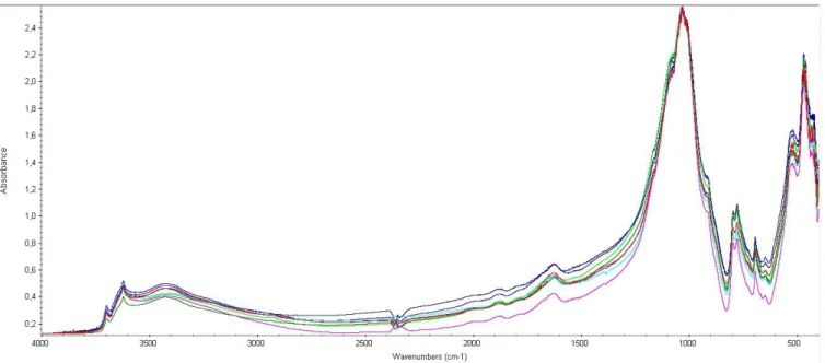
The resulting spectra of the eight layers was first visually compared to each others to check for obvious difference in peaks. As it shows in figure 2, all the spectra peaks at the same wave numbers but with variations in absorption. With the highest peak for all samples is at where silicate bonds are represented. (Si-O). The only clear difference is in the sample of

layer 14 which has a reverse peak at wave number 2350, which is where CO2 is represented.

This was the case of difference in the background and have nothing to do with the sample itself. Therefore all other peaks are relatively identical for all layers, as showen in Fig. 5.

Also, the results were compared statistically by creating a correlation coefficient matrix, which was then used in a hierarchal tree-joining cluster analysis to see which samples cluster together closely and which differs mostly from the rest. The matrix was made using the software WinFIRST.

As both the spectra and the diagram show below, layer 14 seems to differ the most out of the rest. This result contradicts with the initial assumption of similarity between layers 5, 11, and 14.

(14)

Fig. 5: FTIR tree-diagram for the eight layers, using weighted pair-group average linkage rule and squared Euclidean distance to emphasis distances.

14 Fig. 4: FTIR spectra for the eight layers for visual comparison. Peaks seem almost identical. One noticeable difference though is with layer 14, shown in purple.

0.000 0.005 0.010 0.015 0.020 0.025 0.030 0.035 0.040 0.045 14 15 17 16 12 11 10 5

(15)

5.2 XRD

Processing the XRD results proved to be a little bit harder since the patterns were almost identical. All samples peaked at almost the same phases with small variations in intensity. Focusing on the biggest peak differences showed that these exist in the intensity where quartz

(SiO2) , Albite (NaAlSi₃O₈) , and Microcline (KAlSi₃O₈) are detected (Fig. 6); the latter two

are alkali-feldspars and both quartz and feldspar are very common in the near surface quaternary sedimentations in all of the eastern side of Jutland Peninsula (Ohse et al. 1984; BGR n.d.) . As the whole area got affected by similar glacial processes of the last two glacial periods, Weichsel and Saale glaciations (Stephan 2014) .

When the the whole patterns including all of the peaks were processed in Statistica using Fig.6: XRD diffractogram zoomed in to show the main peaks' difference at the angle of detection for albite and microcline.

(16)

Friedman's ANOVA test (analysis of variance) the results were statistically insignificant with a very high error possibility. So the alternative was to mine for the differences in the data. After careful visual examination for the patterns it was decided to focus on the phases peaking between 2θ= 27.5 and 2θ= 68.2 because here the most variations were visible in the diffractogram. Excluding the rest, these peaks and intensities were used to create cluster analysis, and the tree-diagram below shows the results.

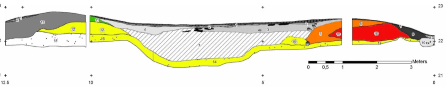
According to the proximity of the crystallinity between the layers shown in the dendrogram in fig. 7. Layers 12 and 15 clustering early, followed by the rest of the layers. The graph indicates high similarity in crystalline structures in the soil samples generally, but a noticeable four clusters are visible with the first and bigger one including layer 12, 15 14, 16, and 17; and the other three clusters include layer 5, layer 10, and layer 11 respectively. With layer 5 clustering somehow close to the biggest clusters mentioned above. The relation created between the layers is illustrated on the cross-section map in fig. 8.

16 Fig. 7: Cluster analysis for the selected XRD results between 2Theta 27.5 and 68.2. Unweighted pair-group Average as a linkage rule and simple Euclidean distance.

(17)

5.3 XRF

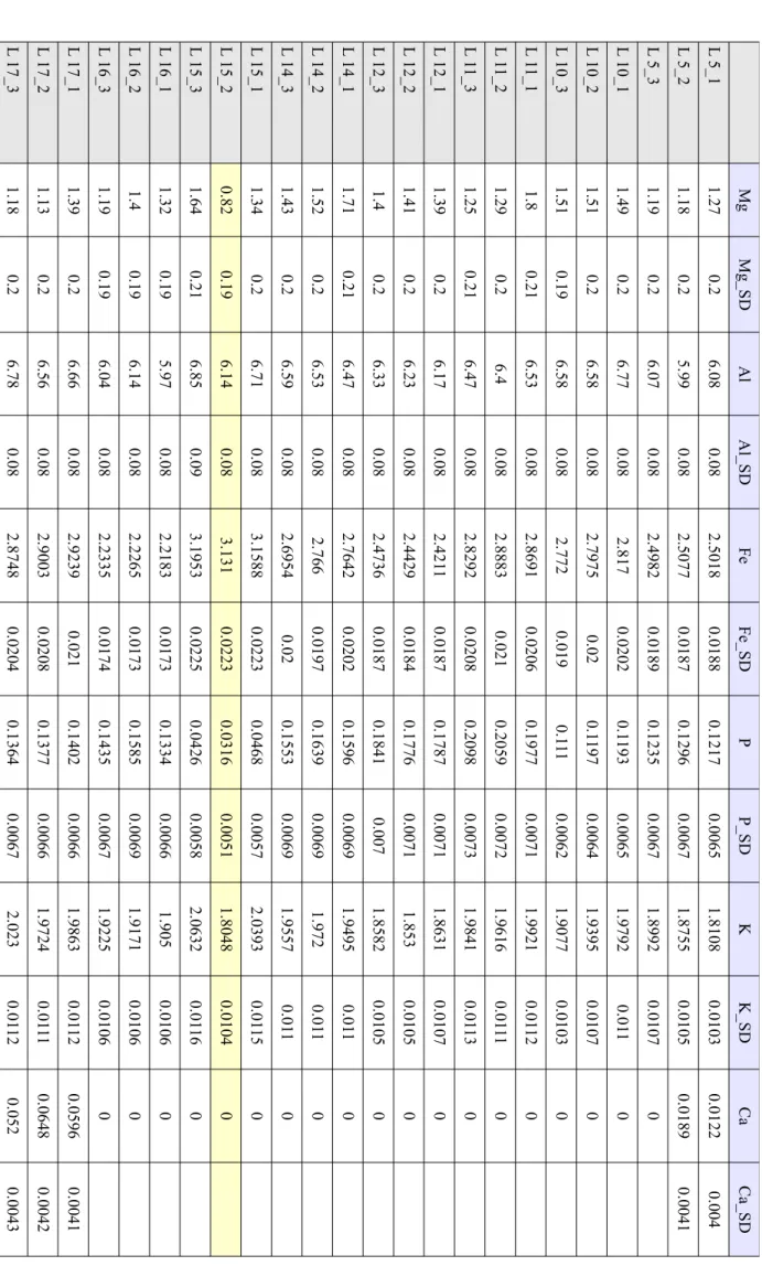
As mentioned earlier, each sample was analysed three times. Hierarchal cluster analysis was, once again, performed to check the similarities and differences between layers. After examining the results' table and a preliminary cluster analysis for the mean detected of the three runs for each sample, the second run of the sample of layer 15 turned out to be an outlier, differing markedly from both the other two runs for the same sample and the rest of the tests of all samples, and clustering lastly with the rest of the tests at a quite far linkage distance. The main difference between test 15_2 and the other two runs for layer 15, namely 15-1 and 15-3 is in the elements Mg, Al, Si, P, K, Ti, and Fe. This difference seems to be more of an error rather than actual value because of the huge difference in comparison to the other two tests of the same sample, see table.1 for the detailed data. This outlier will be ignored in the discussion analysis, mainly for the mentioned difference, but also because that the pirpose of the soil analysis here is mainly to figure the possibility of soil analysis to establish a hypothesis of a relation between the contexts of the site rather than to make final conclusions in this regard, and a single outlier won't affect this process, specifically because of the order

the rest of the tests exhibited (Fig 10)

The diagram below, in Fig. 10, shows the results of the clustering of the all the tests, and Fig. 8: The clusters visible in the XRD test results illustrated on the section map. The map is from Kalmring (in press)

(18)

using all detected chemical components. Another tree cluster analysis was made after excluding the light elements, i.e. elements that has atomic number lesser than 12 (lighter than Magnesium). This exclusion, however, didn't affect the resulted clustering at all, it was thus ignored.

XRF tests shows an expected clustering pattern in the beginning where each layer clusters its three runs together except for the aforementioned test 15_2. Then the two first layers to cluster together are layers 12 and 14. Stopping at linkage distance 3 we have three clusters. The first one includes layers 5 and 10, the second one includes layers 11, 12, 14, and 15; and lastly, layers 16 and 17 together form the third cluster. These three clusters are illustrated with three different colours in Fig. 9 to show the relation between the layers.

18 Fig. 10: Cluster analysis of all the XRF element tests. Unweighted pair-group average as linkage rule, and simple Euclidean distance.

(19)

6. Discussion

The FTIR results didn't provide useful information since all samples included similar chemical bonds in its contents. So the bases for the this discussion will be based on the other two tests run by x-ray diffraction and x-ray florescence.

Both crystallinity analysis and main element analysis showed similarity between some layers and differences between others. The comparison between these two results is illustrated in the schematic figure below (Fig.11) showing the relation between layers in each of XRD and XRF.

Even after excluding layer 15 for showing slight ambiguity in the process, both tests shows a direct and close relation between layers 14 and 12. Also, layers 16 and 17 are close together in both test, expressing similar crystal components with the first mentioned cluster (i.e, layers 14,12, and 15), they show however some difference in the main element components, standing at one end of the spectrum; while layers 5 and 10 stand on the other end, having both similar elements and pretty close crystallinity. Moreover, layer 11 is closely related to the first cluster in the element it contains, although being on the surface, highly exposed to environmental processes, might have been the reason for having different crystalline structure of its components.

According to these results, it is highly possible that the soil used for building the rampart, at least in the early phase of its construction, was brought directly from the inside of the enclosure, thus showing the trench-shaped strata visible in the cross-section in Fig. 3.

Furthermore, the strata related to the burial nearby, namely layers 5 and 10, shows Fig.11: Schematic cross-section map for comparison illustrating the relation between the layers based on the results of both XRF and XRD

(20)

difference in relation to the rest of the layers, which might be an indication of a process separated from the rampart construction both spatially and temporally. However, to make any conclusion in regard of the temporal relation between the burial and the rampart and the “trench” in between needs further sampling and analysis, since there is no clear chronological evidence about any relation of this kind.

This analysis is, nevertheless, exploratory in nature. With such approach, it is important to keep in mind the representativeness of the sample. The sampling wasn't performed with the intention of running soil analysis, under a clear and specific strategy, in order to answer specific questions. Hence, the results of this analysis forms a hypothesis that awaits further verification by applying a statistical sampling plan which extends farther than the excavated area to test if the hypothesis stands still. A general rule in statistics is that “the smaller the relation between variables, the larger the sample size that is necessary to prove it significant” (Lewicki et al. 2006, 9) . Thus, the necessary minimum sample size increases as the magnitude of the effect to be demonstrated decreases. This should be the theoretical base if any further soil analysis is intended in the future. Spatially, the samples here are from the excavated trench, so the results are naturally connected to this specific area; but the rampart extends way beyond to a much bigger area.

To expand the understanding of the spatial, and possibly temporal relation between the contexts and features present in the hill-fort generally, a detailed sampling plan for selected spots along the rampart and areas nearby, whether including burials or not, would help test the predictive validity for the results presented in this paper.

(21)

Mg Mg _S D A l A l_S D Fe Fe _S D P P _S D K K _S D C a C L 5_1 1.27 0.2 6.08 0.08 2.5018 0.0188 0.1217 0.0065 1.8108 0.0103 0.0122 L 5_2 1.18 0.2 5.99 0.08 2.5077 0.0187 0.1296 0.0067 1.8755 0.0105 0.0189 0.0041 L 5_3 1.19 0.2 6.07 0.08 2.4982 0.0189 0.1235 0.0067 1.8992 0.0107 0 L 10_1 1.49 0.2 6.77 0.08 2.817 0.0202 0.1 193 0.0065 1.9792 0.01 1 0 L 10_2 1.51 0.2 6.58 0.08 2.7975 0.02 0.1 197 0.0064 1.9395 0.0107 0 L 10_3 1.51 0.19 6.58 0.08 2.772 0.019 0.1 11 0.0062 1.9077 0.0103 0 L 1 1_1 1.8 0.21 6.53 0.08 2.8691 0.0206 0.1977 0.0071 1.9921 0.01 12 0 L 1 1_2 1.29 0.2 6.4 0.08 2.8883 0.021 0.2059 0.0072 1.9616 0.01 11 0 L 1 1_3 1.25 0.21 6.47 0.08 2.8292 0.0208 0.2098 0.0073 1.9841 0.01 13 0 L 12_1 1.39 0.2 6.17 0.08 2.421 1 0.0187 0.1787 0.0071 1.8631 0.0107 0 L 12_2 1.41 0.2 6.23 0.08 2.4429 0.0184 0.1776 0.0071 1.853 0.0105 0 L 12_3 1.4 0.2 6.33 0.08 2.4736 0.0187 0.1841 0.007 1.8582 0.0105 0 L 14_1 1.71 0.21 6.47 0.08 2.7642 0.0202 0.1596 0.0069 1.9495 0.01 1 0 L 14_2 1.52 0.2 6.53 0.08 2.766 0.0197 0.1639 0.0069 1.972 0.01 1 0 L 14_3 1.43 0.2 6.59 0.08 2.6954 0.02 0.1553 0.0069 1.9557 0.01 1 0 L 15_1 1.34 0.2 6.71 0.08 3.1588 0.0223 0.0468 0.0057 2.0393 0.01 15 0 L 15_2 0.82 0.19 6.14 0.08 3.131 0.0223 0.0316 0.0051 1.8048 0.0104 0 L 15_3 1.64 0.21 6.85 0.09 3.1953 0.0225 0.0426 0.0058 2.0632 0.01 16 0 L 16_1 1.32 0.19 5.97 0.08 2.2183 0.0173 0.1334 0.0066 1.905 0.0106 0 L 16_2 1.4 0.19 6.14 0.08 2.2265 0.0173 0.1585 0.0069 1.9171 0.0106 0 L 16_3 1.19 0.19 6.04 0.08 2.2335 0.0174 0.1435 0.0067 1.9225 0.0106 0 L 17_1 1.39 0.2 6.66 0.08 2.9239 0.021 0.1402 0.0066 1.9863 0.01 12 0.0596 0.0041 L 17_2 1.13 0.2 6.56 0.08 2.9003 0.0208 0.1377 0.0066 1.9724 0.01 11 0.0648 0.0042 L 17_3 1.18 0.2 6.78 0.08 2.8748 0.0204 0.1364 0.0067 2.023 0.01 12 0.052 0.0043

Table. 1: All detected elements in XRF for all layer, including three runs for each sample. The table shows the percentage detected of each

(22)

T i T i_S D Mn Mn_ S D C u C u_S D Z n Z n_S D S r S r_S D L E L E _S D L 5_1 0.3578 0.0202 0.0735 0.0083 0.0022 0.0005 0.0046 0.0004 0.0083 0.0002 56.31 0.21 L 5_2 0.3374 0.02 0.0797 0.0085 0.0023 0.0005 0.0055 0.0004 0.0086 0.0002 56.21 0.21 L 5_3 0.3597 0.02 0.087 0.0085 0.0031 0.0005 0.0063 0.0004 0.0088 0.0002 55.68 0.21 L 10_1 0.3748 0.0203 0.0628 0.0079 0.0033 0.0005 0.0062 0.0004 0.0083 0.0002 54.93 0.21 L 10_2 0.3758 0.0197 0.0658 0.0077 0.0029 0.0005 0.006 0.0004 0.0079 0.0002 55.57 0.21 L 10_3 0.3698 0.0188 0.06 0.0072 0.0025 0.0005 0.0054 0.0004 0.0079 0.0002 55.84 0.2 L 1 1_1 0.39 0.0212 0.1025 0.0091 0.0036 0.0005 0.0067 0.0004 0.0085 0.0002 56.53 0.21 L 1 1_2 0.4168 0.0208 0.1043 0.0093 0.0025 0.0005 0.0067 0.0004 0.0088 0.0002 57.36 0.21 L 1 1_3 0.4069 0.0212 0.1067 0.0092 0.0037 0.0005 0.0066 0.0004 0.0089 0.0002 56.95 0.22 L 12_1 0.3343 0.0195 0.0827 0.0085 0.0027 0.0005 0.0054 0.0004 0.0082 0.0002 56.59 0.21 L 12_2 0.3502 0.0198 0.0682 0.0082 0.003 0.0005 0.0052 0.0004 0.0083 0.0002 56.33 0.21 L 12_3 0.3558 0.0199 0.0919 0.0088 0.0028 0.0005 0.0052 0.0004 0.0079 0.0002 56.51 0.21 L 14_1 0.4307 0.021 0.085 0.0084 0.0038 0.0005 0.0057 0.0004 0.009 0.0002 56.07 0.21 L 14_2 0.4027 0.0203 0.086 0.0084 0.003 0.0005 0.0071 0.0004 0.0089 0.0002 56.15 0.21 L 14_3 0.4095 0.0213 0.0866 0.0087 0.003 0.0005 0.0059 0.0004 0.0085 0.0002 56.21 0.21 L 15_1 0.4695 0.0216 0.0447 0.0075 0.0028 0.0005 0.007 0.0004 0.0087 0.0002 56.64 0.21 L 15_2 0.408 0.0208 0.0564 0.0076 0.0028 0.0005 0.0068 0.0004 0.0089 0.0002 60.14 0.21 L 15_3 0.4567 0.0215 0.0535 0.0075 0.0033 0.0005 0.0075 0.0004 0.0087 0.0002 55.66 0.22 L 16_1 0.3571 0.0202 0.0763 0.0084 0.0037 0.0005 0.0047 0.0004 0.0084 0.0002 56.05 0.21 L 16_2 0.3343 0.0199 0.0851 0.0084 0.0023 0.0005 0.0052 0.0004 0.0082 0.0002 55.54 0.2 L 16_3 0.3442 0.0198 0.0761 0.0084 0.0022 0.0005 0.0045 0.0003 0.008 0.0002 55.96 0.2 L 17_1 0.3938 0.0205 0.081 1 0.0083 0.0036 0.0005 0.0075 0.0004 0.0087 0.0002 56.86 0.21 L 17_2 0.406 0.021 0.0781 0.0083 0.0025 0.0005 0.0072 0.0004 0.0087 0.0002 57.28 0.21 L 17_3 0.4306 0.0203 0.0689 0.0081 0.0022 0.0005 0.0066 0.0004 0.0088 0.0002 56.42 0,21

(23)

Y Y _S D Zr Zr _S D N b N b_S D P b P b_ S D Th Th_S L 5_1 0.0013 0.0001 0.0254 0.0003 0.0012 0.0002 0.0017 0.0002 0 L 5_2 0.0012 0.0001 0.0242 0.0003 0.0013 0.0002 0.0016 0.0002 0 L 5_3 0.0012 0.0001 0.0238 0.0003 0.0013 0.0002 0.0014 0.0002 0.0017 0.0005 L 10_1 0.0015 0.0002 0.0309 0.0003 0.0013 0.0002 0.0015 0.0002 0.0016 0.0005 L 10_2 0.0012 0.0001 0.0306 0.0003 0.0016 0.0002 0.0017 0.0002 0 L 10_3 0.0015 0.0001 0.0305 0.0003 0.0015 0.0002 0.0015 0.0002 0 L 1 1_1 0.0015 0.0002 0.029 0.0003 0.0012 0.0002 0.0017 0.0002 0 L 1 1_2 0.0016 0.0002 0.0297 0.0003 0.0016 0.0002 0.0019 0.0003 0 L 1 1_3 0.0016 0.0002 0.03 0.0003 0.0016 0.0002 0.0019 0.0003 0 L 12_1 0.0013 0.0001 0.0266 0.0003 0.001 1 0.0002 0.0013 0.0002 0 L 12_2 0.0013 0.0001 0.0264 0.0003 0.0012 0.0002 0.0019 0.0002 0.0018 0.0005 L 12_3 0.001 1 0.0001 0.0279 0.0003 0.0016 0.0002 0.0016 0.0002 0 L 14_1 0.0018 0.0002 0.0327 0.0003 0.0018 0.0002 0.0017 0.0003 0 L 14_2 0.0016 0.0001 0.0319 0.0003 0.0019 0.0002 0.0015 0.0002 0.002 0.0005 L 14_3 0.0014 0.0002 0.0321 0.0003 0.0015 0.0002 0.0019 0.0003 0 L 15_1 0.0019 0.0002 0.0273 0.0003 0.0016 0.0002 0.002 0.0003 0 L 15_2 0.002 0.0002 0.0289 0.0003 0.0017 0.0002 0.0018 0.0003 0 L 15_3 0.0021 0.0002 0.0285 0.0003 0.0015 0.0002 0.0022 0.0003 0 L 16_1 0.0015 0.0001 0.0242 0.0003 0.0012 0.0002 0.0017 0.0002 0 L 16_2 0.0014 0.0001 0.0236 0.0003 0.0009 0.0002 0.0016 0.0002 0 L 16_3 0.0012 0.0001 0.0241 0.0003 0.0008 0.0002 0.0022 0.0003 0 L 17_1 0.0014 0.0002 0.0262 0.0003 0.0013 0.0002 0.0023 0.0003 0.0016 0.0005 L 17_2 0.0014 0.0002 0.0266 0.0003 0.0015 0.0002 0.0014 0.0002 0 L 17_3 0.0018 0.0002 0.0257 0.0003 0.0013 0.0002 0.0016 0.0002 0

(24)

U U Si Si _S D A s A s_S D R b R b_S D L ay er 5_1 0 31.42 0.14 0 0.0076 0.0002 L ay er 5_2 0 31.61 0.14 0.0006 0.0002 0.0074 0.0002 L ay er 5_3 0 32.03 0.15 0 0.0074 0.0002 L ay er 10_1 0 31.39 0.14 0.0007 0.0002 0.0078 0.0002 L ay er 10_2 0 30.98 0.14 0 0.0077 0.0002 L ay er 10_3 0 30.79 0.14 0 0.0076 0.0002 L ay er 1 1_1 0 29.53 0.14 0 0.0089 0.0002 L ay er 1 1_2 0 29.31 0.14 0 0.0085 0.0002 L ay er 1 1_3 0 29.74 0.14 0 0.0084 0.0002 L ay er 12_1 0 30.91 0.15 0 0.0075 0.0002 L ay er 12_2 0 31.08 0.14 0 0.0079 0.0002 L ay er 12_3 0 30.74 0.14 0 0.0077 0.0002 L ay er 14_1 0 30.29 0.14 0 0.0084 0.0002 L ay er 14_2 0 30.35 0.14 0.0007 0.0002 0.0082 0.0002 L ay er 14_3 0 30.41 0.14 0 0.0083 0.0002 L ay er 15_1 0 29.49 0.14 0 0.0085 0.0002 L ay er 15_2 0 27.41 0.13 0.0006 0.0002 0.0079 0.0002 L ay er 15_3 0 29.97 0.14 0 0.0086 0.0002 L ay er 16_1 0 31.91 0.14 0 0.0073 0.0002 L ay er 16_2 0 32.15 0.14 0 0.0073 0.0002 L ay er 16_3 0.001 1 0.0003 32.04 0.14 0 0.0071 0.0002 L ay er 17_1 0 29.44 0.14 0 0.0082 0.0002 L ay er 17_2 0 29.4 0.14 0.0005 0.0002 0.0083 0.0002 L ay er 17_3 0 29.98 0.14 0.0009 0.0002 0.008 0.0002

(25)

7. References

Antoniassi, J., Kahn, H., Ulsen, C., & Tassinari, M.L. 2012. Prediction of Mineral Processing Behavior of Bauxite Ores by XRD Cluster Analysis. In M. A. T. M. Broekmans (ed)

Proceedings of the 10th International Congress for Applied Mineralogy (ICAM), 9–16.

Springer Berlin Heidelberg Available at: http://dx.doi.org/10.1007/978-3-642-27682-8_2.

BGR. Geologische Übersichtskarte 1 : 200 000, Blatt CC 1518 Flensburg. Bundesanstalt für

Geowissenschaften und Rohstoffe. Available at:

http://www.bgr.bund.de/EN/Themen/Sammlungen-Grundlagen/GG_geol_Info/Karten/Deutschland/GUEK200/Texte/Flensburg.html? nn=2032520 [Accessed May 1, 2015].

Bish, D.L., & Post, J.E. 1989. Modern powder diffraction. Washington, D.C.: Mineralogical Society of America.

Butler, D.H., & Dawson, P.C. 2013. Accessing Hunter-Gatherer site structures using Fourier transform infrared spectroscopy: applications at a Taltheilei settlement in the Canadian Sub-Arctic. Journal of Archaeological Science 40(4): p.1731–1742.

Castro, K. et al. 2007. Vibrational spectroscopy at the service of industrial archaeology: Nineteenth-century wallpaper. TrAC Trends in Analytical Chemistry 26(5): p.347–359. Dobat, A.S. 2008. Danevirke Revisited: An Investigation into Military and Socio-political Organisation in South Scandinavia (c AD 700 to 1100). Medieval Archaeology 52(1): p.27–67.

Gauthier, G., Burke, A.L., & Leclerc, M. 2012. Assessing XRF for the geochemical characterization of radiolarian chert artifacts from northeastern North America.

Journal of Archaeological Science 39(7): p.2436–2451.

Grupe, G., von Carnap-Bornheim, C., & Becker, C. 2013. Rise and Fall of a Medieval Trade Centre: Economic Change from Viking Haithabu to Medieval Schleswig Revealed by Stable Isotope Analysis. European Journal of Archaeology 16(1): p.137–166.

Hjulström, B., & Isaksson, S. 2009. Identification of activity area signatures in a reconstructed Iron Age house by combining element and lipid analyses of sediments. Journal of

Archaeological Science 36(1): p.174–183.

Holmquist, L. 2002. Patterns of settlement and defence at the proto-town of Birka, Lake Mälar, eastern Sweden. In Scandinavians from the Vendel period to the tenth century

2002.Studies in historical archaeoethnology, 153–175. Woodbridge, Boydell Press

Holmquist, L., & Kalmring, S. 2012. Stadslika handelsplatser med borgar - Hedeby och Birka. Populär arkeologi 29(3): p.4–8.

Kalmring, S. In press. Hedeby Hochburg- Theories, State of research, and dating. Offa.

(26)

Fornvännen 105(4): p.281–290.

Kalnicky, D.J., & Singhvi, R. 2001. Field portable XRF analysis of environmental samples.

On-site Analysis 83(1–2): p.93–122.

Kjellin, J. 2004. XRF-analys av förorenad mark. undersökning av felkällor och lämplig

provbearbetning. Examenarbete. Uppsala: Uppsala Universitet.

Lewicki, P., & Hill, T. 2006. Statistics: methods and applications. Tulsa, OK. Statsoft. Available at: http://bib.convdocs.org/docs/5/4212/conv_1/file1.pdf [Accessed February 6, 2015].

Linderholm, J., & Lundberg, E. 1994. Chemical Characterization of Various Archaeological Soil Samples using Main and Trace Elements determined by Inductively Coupled Plasma Atomic Emission Spectrometry. Journal of Archaeological Science 21(3): p.303–314.

Moore, T.R., & Denton, D. 1988. The role of soils in the interpretation of archaeological sites in Northern Quebec. In J. L. Bintliff, D. A. Davidson, & E. G. Grant (eds) Conceptual

issues in environmental archaeology, 25–37. Edinburgh: Edinburgh University Press

Ohse, W., Matthess, G., Pekdeger, A., & Schulz, H.D. 1984. Interaction water—silicate minerals in the unsaturated zone controlled by thermodynamic disequilibria. In

Hydrochemical Balances of Freshwater Systems: Proceedings of the Uppsala Symposium September 1984. IAHS-AISH Publication, Available at:

http://www.researchgate.net/profile/Horst_Schulz2/publication/256474645_Interaction

_water-silicate_minerals_in_the_unsaturated_zone_controlled_by_thermodynamic_disequilib ria/links/0c960522f416285d9f000000.pdf [Accessed May 1, 2015].

Parsons, C. et al. 2013. Quantification of trace arsenic in soils by field-portable X-ray fluorescence spectrometry: Considerations for sample preparation and measurement conditions. Journal of Hazardous Materials 262: p.1213–1222.

Roche, D., Ségalen, L., Balan, E., & Delattre, S. 2010. Preservation assessment of Miocene– Pliocene tooth enamel from Tugen Hills (Kenyan Rift Valley) through FTIR, chemical and stable-isotope analyses. Journal of Archaeological Science 37(7): p.1690–1699. Squires, K.E., Thompson, T.J.U., Islam, M., & Chamberlain, A. 2011. The application of

histomorphometry and Fourier Transform Infrared Spectroscopy to the analysis of early Anglo-Saxon burned bone. Journal of Archaeological Science 38(9): p.2399– 2409.

Stephan, H.-J. 2014. Climato-stratigraphic subdivision of the Pleistocene in Schleswig-Holstein, Germany and adjoining areas. E&G Quaternary Science Journal 63: p.3–18. Wilson, C.A., Davidson, D.A., & Cresser, M.S. 2008. Multi-element soil analysis: an assessment of its potential as an aid to archaeological interpretation. Journal of

Archaeological Science 35(2): p.412–424.

Xu, Z. et al. 2001. Quantitative mineral analysis by FTIR spectroscopy. Internet Journal of

(27)

Vibrational Spectroscopy [www.ijvs.com]. Vol 5, Issue 1. Available at:

http://www.ijvs.com/volume5/edition1/section2.html [Accessed January 4, 2015].

List of figures

Fig. 1: Trench 2012 showing layer 14 where the scale is positioned. Photo toward the south. (Kalmring, In press)...1

Fig. 2: Danevirke's location in Schleswig-Holstein marked in white rectangle in the first map to the left. Its location in relation to Hedeby in the upper map to the right. And lastly, the rampart of Hedeby in relation to the hill-fort of Hedeby (white polygon) in the lower map to the right. Maps are from Open Street Maps, processed in ArcGIS 10.1...4

Fig. 3: Profile and plan illustration of the 2012 excavation trench. Adapted fromSven Kalmring (In press). Layers that are tested in this paper are marked with green squares around its number...8

Fig. 4: FTIR spectra for the eight layers for visual comparison. Peaks seem almost identical. One noticeable difference though is with layer 14, shown in purple...14

Fig. 5: FTIR tree-diagram for the eight layers, using weighted pair-group average linkage rule and squared Euclidean distance to emphasis distances...14

Fig.6: XRD diffractogram zoomed in to show the main peaks' difference at the angle of detection for albite and microcline...15

Fig. 7: Cluster analysis for the selected XRD results between 2Theta 27.5 and 68.2. Unweighted pair-group Average as a linkage rule and simple Euclidean distance...16

Fig. 8: The clusters visible in the XRD test results illustrated on the section map. The map is from Kalmring (in press)...17

Fig. 9: The three clusters resulted from the XRF tests. The section map is from Kalmring (in press)...17

Fig. 10: Cluster analysis of all the XRF element tests. Unweighted pair-group average as linkage rule, and simple Euclidean distance...18

Fig.11: Schematic cross-section map for comparison illustrating the relation between the layers based on the results of both XRF and XRD...19

(28)

Soil Analysis for samples from the hill-fort of Hedeby