Is there a relationship between oil prices and house price inflation?

(1)

Is there a relationship

between oil prices and

house price inflation?

BACHELOR THESIS WITHIN: Economics NUMBER OF CREDITS: 15hp

PROGRAMME OF STUDY: International Economics and Civilekonom Programmet

AUTHOR: Amanda Magnusson & Lina Makdessi JÖNKÖPING May 2019

(2)

(3)

Bachelor Economics

Title: Is there a relationship between oil price and house price inflation? Authors: Magnusson, A. and Makdessi, L.

Tutor: Kristofer Månsson Date: 2019-05-20

Key terms: Energy economics, House price inflation, Oil price, House price turning points, Trade status, Linear regression model, Conditional logit model

Abstract

The purpose of this thesis is to investigate further whether oil price has an effect on house price inflation and additionally if it has a link to house price turning points. The methodology is grounded on the previous research paper made by Breitenfellner et al. (2015). The results are based on quarterly data from the countries; Finland, Denmark, Norway and Sweden through the time span of 1990-2018. A linear fixed regression model was performed including the explanatory variables of monetary policy and credit developments, macroeconomic fundamentals, housing market variable and demographic variables. Secondly, a logit model was used to identify a relationship between oil price and house price turning points. The model used misalignment made from GDP per capita and real interest rate.

The empirical analysis confirms that there is a positive relationship between oil prices and house price inflation. This evidence contradicts a major share of previous research papers (see Bernanke, 2010; Kaufmann et al., 2011). However, there are also some previous papers (see Yiqi, (2017); Antonakakis et al., 2016) and theoretical linkages in line with a positive correlation. Concerning, the oil price and house price inflation no empirical significance was found regarding their relationship. For future research, one could include regional aspects for the purpose of controlling for geographical differences.

(4)

Table 1. Presentation of the explanatory variables. _______________________________________________ 12 Table 2: Descriptive statistics concerning the chosen variables._____________________________________ 13 Table 3. Results of Brent crude oil price, lagged house price inflation and other determinants of the dependent

variable. ________________________________________________________________________________ 21

Table 4. Identified turning points for house prices. _______________________________________________ 24 Table 5. Estimation results for conditional logit models of house price turning points. ___________________ 25 Table 6. Oil price effects on house price inflation presented for each country separately. _________________ 27

APPENDIX

Table A 1: Descriptive statistics of the variables used in the empirical models. _________________________ 32

Table A 2: Long-run elasticity estimates of misalignment __________________________________________ 32

Table A 3: Hausman test ___________________________________________________________________ 33

Table A 4: Augmented Dickey Fuller unit root test _______________________________________________ 33

Table A 5: Simple regression model, first difference house price inflation and the lag of the difference house

price inflation. ___________________________________________________________________________ 34

Table A 6: Variance Inflation Factor__________________________________________________________ 34

Table A 7: White’s heteroscedasticity test with cross-terms ________________________________________ 35

Table A 8: Pooled linear regression model _____________________________________________________ 35

(6)

1. Introduction

In this paper, we will analyse the role played by oil price on house price inflation. The focus will lay on explaining if there is a relationship between oil and house prices. Additional analysis will be made concerning the role of oil price on historical house price turning points. Investigating the probability of a change in oil price causes house price fluctuations, considering price peaks. We will also examine whether there are differences between exporting and importing countries, in terms of the oil price effect on housing. The final results indicate that there is a relationship between oil and house prices, however we find no significant evidence linking oil price to house price turning points and the trading status of each country respectively.

Earlier research on the topic of energy price present differences in their findings regarding the relationship with house prices, where some suggest that there is a positive relationship while others suggest the opposite. The majority of previous research provides evidence for a negative linkage between oil price and house price. This includes the study of Bernanke (2010), who explains that the crude oil shock build-up from 2000 to the mid-2008, occurred in coexistence with the emerge of the US subprime mortgage crisis, which led to the most severe financial crisis since the Great Depression. The results of Kaufmann et al. (2011) are in line with Bernanke (2010) research suggesting that the oil shock had a direct role in the 2008 financial crisis. This can also be supported by the study by Leamer (2007), explaining that energy inflation and house price turning points are identified as important determinants of recessions. He also presented evidence that shocks in the housing sector was the result of eight out of nine post-war recessions. Further evidence regarding US recessions are presented by Hamilton (2005), who states that nine out of ten recessions were to follow an oil price shock. Breitenfellner et al. (2015) investigated the coincidence of the financial crisis of 2007-09 occurring at the same time as the oil shock. The reached conclusion was such that increases in energy price inflation raised the probability of the occurrence of house price turning points. Hence, causing a crisis in the house price market.

On the contrary, a few papers suggest a positive relationship between the oil price and the house price have been identified. The first one is presented by Antonakakis et al. (2016),

(7)

where they examine the dynamic co-movements between housing and oil market returns in the U.S. over the period of 1859 to 2013. They find evidence suggesting that the co-movements are consistently negative. However, they also provide evidence that in the 19th_{century as the U.S. economy experienced several recessions, the correlations of oil} and house prices were positive. Another positive linkage has been made by Yiqi (2017), who studied if oil prices have a significant impact on the housing prices in the Norwegian market. The results showed that oil prices have a positive relationship with the house price market in Norway.

On the topic, we found several papers relating monetary policies to house price inflation (see Fuss and Zietz, 2016; Bjørnland and Jacobsen, 2009; Leamer, 2007). It is also mentioned by Breitenfellner et al. (2015), that there is not much research in this area. This sparked our interest to further investigate the role played primarily by oil price. In contrast to using energy inflation, as Breitenfellner et al. (2015) use, we identified oil as the primary source of energy inflation and to see if the results would be any different when isolating the effects of oil.

Our hypothesis is that there is a significant relationship between the oil price and house price inflation. However, as previous research provide evidence for both positive and negative linkages, there is an uncertainty to which sign our sample estimate will take on. The expected results according to theory (described below) might take on positive or negative signs. However, the negative signs have been dominating in previous studies. The interest of this paper is to see which channel that dominates the relationship between oil prices and house price inflation in a time where we move away from a highly intense oil consumption pattern. Additionally, we also investigate if the trade status (exporting or importing oil) of the sample have any dominant effect on house price and we believe that there is some difference.

The theoretical linkages presented by literature can be attributed by six channels underlying the relationship of oil price and house price inflation. First, it is suggested that household disposable income, consumption and investment (essentially housing) is dampened due to adverse direct and indirect increases in the oil price (European Central Bank, 2010). Second, that quantity and supply adjustments on the supply side can be

(8)

affected as an increase in the oil price affect construction and building costs, hence leading to a positive relationship between the variables. Third, the tightening reaction of increased oil prices on monetary policy puts pressure on the interest rate, indirectly reducing the liquidity in the housing market as well as the corresponding aggregate demand (International Monetary Fund, 2008), causing a negative correlation. Fourth, when inflation expectations are rising, investors become keener on investing in the oil and housing market as they serve as a hedge against inflation, which indicates that there is a positive relationship between them. Second to last, the trading status of the economy is an important determinant of how the effects of oil price will affect the housing market within the country (Kilins et al., 2017). Lastly, explaining there might be lagging impacts of third common factors on both oil and housing price, such as economic growth or monetary policy (see Frankel, 2008; Bjornland and Jacobsen, 2009; Goodheart and Hofmann, 2008). As one can understand, there are several positive and negative relations identified between oil price and house price inflation in the theoretical section. The result will identify if the relationship is positive or negative and hence explain which theoretical linkages that are the dominant.

The empirical test of whether there is a relationship between oil prices and house price will be performed using a panel data set of quarterly data, gathered from OECD, Thomson Reuters data stream and the World Bank. The evaluated countries include a sample of Denmark, Finland, Norway and Sweden, and will cover the time-period 1990 until 2018. Including several proxies to account for relevant monetary policy and credit developments, macroeconomic fundamentals, housing market and demographic variables. We also account for house price misalignment, which is estimated by secondary data. Our results confirm that changes in oil price have a significant effect on house price inflation. However, when controlling specifically for the effects of oil price on house price turning points there were no indications of such relation. Including the empirical results from the individual countries, respectively, there is no noticeable difference in terms of exporting and importing oil economies, as theory propose there would be. The layout structure of this research paper is: Section 2 presents the relevant literature and the theoretical linkages. Section 3 describes the data. Section 4 explains the methodology used in the paper. In Section 5 the empirical results are presented and the

(9)

discussed in relation to the theoretical evidence. Under Section 6 conclusions will be drawn.

(10)

2. Theoretical Background

This section will explain several theoretical linkages between oil prices and the house price inflation made by existing literature. A summarization of these linkages will be put forward in the following channels: (2.1) income and demand, (2.2) energy related building cost, (2.3) monetary policy, (2.4) asset price, (2.5) trading status: exporting vs importing differences and (2.6) via reversed causality or omitted factors.

2.1. Income and Demand

The European Central Bank (2010) explain the impact of energy price activity by dividing the effects into three different sub-groups; terms-of-trade, demand- and supply-side effects. The terms-of-trade effects origins from the increase in the import prices of energy, this leads to an increase in total import price relative to export prices. Hence, an oil price increase in the importing country causes a reduction in purchasing power and wealth of households. This will possibly trigger a reduction in the households’ savings-rates and thereby also reduce the consumption and investment (in housing).

The second effect, the (aggregated) demand-side, which arise from the impact of energy prices on inflation (European Central Bank, 2010). As prices increases, the households’ real disposable income and, therefore, consumption are reduced. In an ideal economy, under perfect competition in the labour and product markets, a rise in energy prices would only lead to a relative price change, which would later be compensated by substitution for less-energy intensive products. Although, rigidities suggest otherwise. The effects of energy price are decomposed into first-round and second round effects. The first-round effects refer to the impact of changes in primary prices of energy (e.g. oil and gas) on consumer energy prices, and the impact of changes in consumer prices that occur as energy prices impact on producer and distribution prices. However, a one-off price increase of the first-round effects only contribute to an increase in the price level and, hence, no lasting inflationary effects. Whilst, the second-round effect capture the reactions of wage and price-setters to the first-round, as they want to keep their real wages and profits unchanged. The energy price movements are magnified and extended in the second-round effects and, thus, the impact on wages may be further reinforced by additional upward pressure on the price level. As the price-setters, the employers, want to pass rising labour costs on to consumer prices as they want to maintain the real value

(11)

of their profits, which are already penalised by higher input prices. Altogether, this can cause higher inflation expectations to become embedded in the wage and price-setting process, which can put the price stability of the economy to become endangered.

Lastly, there is the supply-side effects which arise from the input costs of the production process (European Central Bank, 2010). Thus, increases in energy price will lead to higher production costs, and in the short-term firms may react to the shock either by pricing or production behaviour, this by reduction of profit margins or increasing the selling price. This causes not only the consumption and quantities produced to fall but will also cause wages, employment and investment to go down. All this concludes that an increase in the oil price has the tendency to depress income, by decreased purchasing power, profit squeeze and increasing the unemployment rate.

To summarise, the effects of terms-of-trade, demand-side effects provide evidence for a negative relationship between the oil price and the house price. Concerning the supply side effects, there are evidence of both positive and negative relationships. The positive indicating that higher production costs as a consequence of rising oil price, can cause an increase in selling prices by firms in the short term. It can also be explained as a negative relationship, as increases in oil price can potentially depress income, squeeze profits and increase the unemployment rate.

The discussed effects above can partly explain the correlation between household consumption of energy and the mortgage delinquency rate. Kaufmann et al. (2011) suggest there is a relationship between the rising oil prices in terms of household expenditure on energy and the mortgage delinquency rate. They state that the rise in oil prices spread to other form of energy as well, e.g. natural gas and electricity. Since the own-price elasticity of demand for energy consumption is relatively small for households, rising energy prices cause households to spend a larger fraction of their income on energy, as oil prices increases. Also, as consumers do not place much emphasis on energy use when purchasing a home an unanticipated rise in energy prices causes households to fall behind on their mortgages, which increase mortgages delinquency rates.

(12)

However, not only do changes in energy price affect spending patterns of households, as the effect of real consumption aggregates have been questioned, other research provides evidence for direct effects in precautionary savings and the operating cost of energy-using durables as well (Edelstein and Kilian, 2009). Edelstein and Kilian (2019) explain that when consumers become pessimistic about the state of their personal financial situation as well as the overall economy when prices increases, this leads to concerns about the current buying situation as they expect the future economic condition to worsen. This due to unexpected losses in the purchasing power caused by falling oil prices have a negative relationship with the consumer expectations. Hence, deteriorating consumer confidence is likely to be an important link in the relationship between energy price shocks and household consumption (and investment).

2.2. Energy Related Building Cost Channel

The use of energy in terms of residential buildings can be divided into the building-stage and the operating-stage. The building-stage use of energy concerns the construction process, where firstly raw materials needed to be extracted and processed to a finished good and later transported to the construction location. Secondly, the process of building the residential demands labour and machines to finalise the build and not to be forgotten the process will repeat itself whenever maintenance or reparation is necessary. The operating-stage is the energy usage of heating and cooling to uphold a living- and working-standard.

A recognized positive effect of rising oil prices in terms of increasing construction and operational building costs, relating to house price increase, is presented by Antonakakis et al. (2016). This can also be partly explained by the supply-side effects of the previous section (2.1 Income and demand channel). It goes as follows, as construction and operational building costs rise as a consequence of increasing oil prices, the results might be such that is causes the supply of houses to decrease. This can in turn affect the price of housing by pushing up the price.

The energy related building cost channel also has substantial value to the overall energy consumption. According Quigley (1984), service commercial, industrial and residential structures accounts for 40% of the energy consumption in the US and 50% of this energy

(13)

is consumed by the residential sector. Hence, the negative effect of rising oil prices causes sizable effects on housing demand and prices. Further Quigley (1984) examines the services households derive from the dwelling (residential) they inhabit and consider the demand for residential energy as a factor input.

2.3. Monetary Policy

According to the International Monetary Fund (2008), changes in interest rate can affect the domestic demand for housing by directly targeting household spending plans through changes in cost and availability of credit. The indirect effects cause changes in house prices. International Monetary Fund (2008) also explains that in an analysis made on the Netherlands, looking at the effect of tightening monetary policies on housing dynamics the results demonstrate signs of contained housing dynamics in the aspect of house prices. The conclusions of the research were drawn as to indicate that house prices show more responsiveness to monetary policy changes, in the cases where countries with (a higher flexible) mortgage has been deregulated. In the US, the monetary policy is favoured in the more flexible and developed housing finances.

Edelstein and Kilian (2009) discusses that if regulations are made for oil prices to consequently rise per year and the consumption remains consistent, in the end household consumption will at large part be affected due to the decrease in real GDP. One will see a lower consumption on all household hence indirectly affect the house prices due to decrease on the demand side.

The results provided by Mishkin (2007) do align with the previously mentioned research. Monetary policy is a factor influencing housing prices to some extent, in both cases of an economic instability and stability in a country. However, the concerns made of the author is the extent of the influence.

2.4. Financial Market

On the asset market, housing related securities compete with energy securities. As the price for energy increases the housing securities sector becomes more vulnerable, since investors are drawn to commodity developments. However, when inflation expectations are rising investors become keener on investing in these markets as they serve as a hedge against inflation, which postulates a positive relationship between oil and house prices

(14)

compared to previous statement (Breitenfellner et al., 2015). The evolution of US house price boom is explained by Caballero at al. (2008) and El-Gamal and Jaffe (2010), stating that the consequence of the petro-dollar recycling that took place post the subprime crisis. As emerging countries grew quickly, the associated price increase in commodities caused capital to flow towards the US in search for liquid financial instruments (see Higgins et al. 2006). Evidence for this behaviour is presented by Caballero et al. (2008), explaining that the negative correlation between oil and stock prices between July 2007 and June 2008 was exceptionally strong. The after math of the bursting house price bubble, is that the interaction between financial, energy and housing markets continues to have an important role in explaining the global developments. As the crash worsened the scarcity of assets, lead to a large positive demand shock in the markets for commodities, especially for oil (Breitenfellner et al., 2015).

2.5. Trading Status: Net Exporter vs Net Importer

Killins et al. (2017) suggest that there is a difference in whether an economy imports or exports and hence that the trading status matters. Presenting evidence that the reaction of the housing market due to shifts in oil prices have much to do with the primary reason of the oil shock (supply or demand). By implementing structural VAR models observing two economies, an oil exporting (Canada) and an oil importing (U.S), they concluded that shocks originating from oil supply have no apparent effect on housing prices. On the other hand, (aggregated) demand shocks have a statistical effect on house prices in peaks and troughs, although they are economically negligible. Killins et al. (2017) concludes that both oil supply and (aggregate) demand shocks do not have any significant effect on the housing pricing. However, other oil-specific shocks (precautionary demand) have a predominant effect on housing prices in Canada (exporter) compared with the U.S. (importer) housing market. As a result, rising house prices capture the rises in uncertainty in regard to future supply shortfalls and hence the increases in oil price volatility. The consequences of the shock affected the housing market variance by 5% in the net exporting country and by 1,5% in the net importing country. Khiabani (2015) confirms the findings by Killins et al. (2017), that the relationship between house prices and a world oil shock appears stronger in net exporting countries compared to net importing.

(15)

The theoretical framework above provides evidence that the effects of oil price shocks on the housing market is distinguished by the trading status of the economy. Further, investigation is presented by Filis and Chatziantoniou (2014) as their results indicate that the inflation of exporting or importing oil countries has a significant positive relation to the occurrence of an oil price shock. Also, according to Jung and Park (2011), the positive effects of aggregate demand shock in oil exporting economies can be explained by an increase in wealth, consumption and investment due to the increase in the oil price.

2.6. Omitted Factors or Reversed Causality

The impact of oil and house prices may be influenced by global liquidity, monetary policy, regulation and supervision of the financial markets and some other proposed cyclical dynamics, this can cause the variables to appear causal when they are created by a third factor. Frankel (2008) have documented that globally accommodative monetary conditions drive commodity prices. Commodity prices are affected by the interest rate in terms of its effects on aggregate demand, inflation and the incentives for producers to postpone extraction.

Concerning the monetary policy channel, empirical evidence presented by Bjornland and Jacobsen (2009) suggest that the role of house prices in the monetary transmission mechanism is increasing. Their evidence of the relationship is constructed from a structural VAR model. Recent crises have increased the focus, especially among central banks, on asset price developments primarily due to the collateral role of asset (dwelling) prices. Although central banks inflation targeting has managed to keep inflation in check, they have not been able to control the negative real effect of the bursting of asset prices, which can be an important source of macroeconomic fluctuations. Since housing play a dual role, firstly as a store of wealth and second as a durable consumption good, they could work as transmitters of shocks. This since they react quickly to news as they affect the wealth of homeowners directly. Resulting in that this type of asset may be an important indicator of the monetary policy stance. Hence, the implementation of an efficient monetary policy strategy may be dependent on the understanding of the transmission mechanism of asset prices. Evidence of a multidirectional link between house prices, monetary- and macroeconomic variables have been established by Goodheart and Hofmann (2008). They suggest that the effects on shocks to money and

(16)

credit on house prices are stronger when house prices are booming than otherwise. In contrast, the results presented by Bernanke (2010) finds that the linkages of the past decade are rather weak, between monetary policies and house price changes.

Both Hamilton (2009) and Kilian (2009) suggest that the global demand has an important role in explaining oil price developments, and that this demand could come from house price wealth effects (Leamer, 2007).

(17)

3. Data Description

The data used in this thesis is gathered from the OECD statistical database (Organisation for Economic Co-operation and Development), with the exception of the oil prices which are collected from Thompson Reuters data-stream and GDP per capita growth which is collected from the World Bank. The time-series contains quarterly observations 1990:1 to 2018:3, covering the countries; Denmark, Finland, Norway and Sweden. One limiting factor concern the timeframe, where the demographic variables and the credit growth variable are collected per annual instead of quarterly. This is due to missing data. We analyse the sample on a panel dataset, as it allows us to control for variables that normally cannot be observed or measured. Hence, it accounts for individual heterogeneity (Gujarati and Porter, 2009). The collected data was chosen on the basis of our research question and the theoretical framework, presented in section 2. The dependent variable is the house price inflation and the independent variables are oil price, measured by the Brent crude oil price index, and the other determinants of house price changes. The other determinants of house price changes are presented in Table 1, where they are divided into different variable proxies for simplification purposes. The descriptive statistics for each variable are then presented in Table 2.

Table 1. Presentation of the explanatory variables.

Variable proxies Explanatory variables

Monetary policy and credit developments Credit growth

Interest rate changes Macroeconomic fundamentals GDP per capita growth

Current account balance Housing market variable Investment in housing

Demographic variables Share of working age population Population growth

(18)

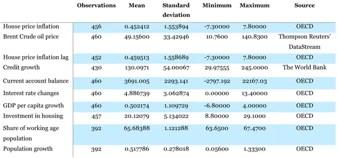
Table 2: Descriptive statistics concerning the chosen variables.

Observations Mean Standard deviation

Minimum Maximum Source

House price inflation 456 0.452412 1.553894 -7.30000 7.80000 OECD Brent Crude oil price 460 49.15600 33.42946 10.7600 140.8300 Thompson Reuters’

DataStream House price inflation lag 452 0.459513 1.558689 -7.30000 7.80000 OECD Credit growth 430 130.0971 54.00067 29.97555 245.0000 The World Bank Current account balance 460 3691.005 2293.141 -2797.192 22167.03 OECD Interest rate changes 460 4.886739 3.062874 0.00000 13.40000 OECD GDP per capita growth 460 0.502174 1.109729 -6.80000 4.00000 OECD Investment in housing 457 20.12079 5.134022 8.80000 29.1000 OECD Share of working age

population

392 65.68388 1.121288 63.6500 67.4700 OECD Population growth 392 0.517786 0.278018 0.05600 1.33300 OECD

House Price Inflation [Price]: The measure of price is based on OECD’s housing price index, an index which measures the development of the price of housing with 2015 being the base year. The price is measured in real terms, which is given by the ratio of nominal price to the consumers’ expenditure deflator in each country, which is seasonally adjusted, from the OECD national accounts database.

Brent crude oil [Price]: The measure of oil price is gathered from Thomson Reuter data-stream and is based on Brent crude which is a major trading classification of sweet light crude oil that serves as a benchmark price for purchases of oil worldwide. The measurement is USD per barrel. The mean value for the sampled countries is of 49.2 USD per barrel and the standard deviation is 33.4 USD.

Credit growth [percentage terms]: The measure of credit growth is based on The World Bank estimates, which is defined as domestic credit to the private sector by banks as a percentage of the total GDP. The index is measured as an annual percentage.

Interest rate [percentage terms]: Long-term interest rates gathered from OECD, referring to government bonds maturing in ten years. They are derived from an average of daily rates measured in percentage terms. The rates are mainly determined by the price charged by the lender, the risk from the borrower and the fall in the capital value. They are implied

(19)

by the prices at which the government bonds are traded on financial markets, not the interest rates at which the loans were issued.

GDP per capita growth [percentage terms]: The collected data originate from the OECD website. It is defined as a quarterly measure of GDP divided by the population of the chosen country. It is represented as a percentage since it shows the average growth level for the index.

Current account balance [USD]: The data is collected from OECD and is defined as the record of a country’s international transactions with the rest of the world. It is measured in USD at a quarterly frequency.

Investment in housing [percentage terms]: The measure of investment in housing is based on OECD’s investment by asset index, where housing investment is measured as a percentage of total gross fixed capital formation (GFCF).

Share of working age population [percentage terms]: The share of working age population data is also gathered from OECD, where they define the share of the population as those aged 15 to 64. This indicator is measured as an annual percentage of population.

Population growth [percentage terms]: Population growth is measured in terms of annual growth rate, where the measure is obtained from OECD and they define population as all nationals present in or temporarily absent from a country. Growth rates are the annual changes in population resulting from births, deaths and net migration during the year.

(20)

4. Method

4.1 Linear Regression Model

To begin with, a model had to be established to answer the research question regarding if there is a relationship between the oil price and house price inflation. The model should primarily focus on the role played by oil prices as a determinant of the overall house price changes. The model had to incorporate the dependent variable: house price inflation, and the independent variables; the oil price and the other chosen determinants explaining house price inflation changes.

Breitenfellner et al. (2015) used a fixed effect model when estimating the relationship of house price inflation, including both a country- as well as a time fixed effect. Equation 1 present the overall role of house price inflation by Brent Crude oil price and other determinants of house price inflation:

Equation 1: _Δ𝑝ℎ_𝑖𝑡 _{= 𝛾}₀_{+ 𝜌Δ𝑝ℎ}_{𝑖𝑡−𝑡}_{+ 𝜇∆𝑝𝑜}_𝑖𝑡 _{+ 𝑍}_𝑖𝑡_{𝜃 + Υ+𝜀}_𝑖𝑡

∆𝑝ℎ𝑖𝑡 denote the house price inflation and ∆𝑝𝑜𝑖𝑡 the Brent crude oil price. The vector 𝑍𝑖𝑡 summarize the other house price determinants, which are the following variable proxies; monetary policy and credit developments (credit growth, interest rate changes), macroeconomic fundamentals (GDP per capita growth), housing market variable (investment in housing) and demographic variables (share of working age population, population growth). The variable, _{Υ, accounts for the time trend. The error term, 𝜀}_𝑖𝑡, is assumed to be composed by a country and year fixed effect which is assumed to fulfil the standard assumptions required in linear regression models.

Testing whether we can follow the same structure Breitenfellner et al. (2015), we constructed a Hausman’s test. The null hypothesis of this test favours the random effects model, while the alternative hypothesis favours the fixed effects model.

The next step regards detection of stationarity among the individual data time-series. It is crucial that our time-series does not follow a nonstationary pattern, which possesses the statistical properties such that the variance and mean change over time. An ideal

(21)

time-series has both constant variance and mean over time, hence it is simpler to predict future values based on current data. In order to test for stationarity, we ran the Augmented Dickey-Fuller (ADF) unit root test, which test the null hypothesis that a unit root is present in a time series sample and the alternative hypothesis is that the time-series is stationary (Dickey and Fuller, 1979).

Further, tests regarding heteroscedasticity and multicollinearity will be performed. Detecting for multicollinearity a variance inflator factor test (VIF), where a value of VIF greater than 10 is assumed to detect severe multicollinearity (Gujarati, 2009). According to Gujarati (2009) a rule of thumb is that if the value of VIF is greater than 10, multicollinearity is severe. On the other hand, we also test for heteroscedasticity through a White’s heteroscedasticity test (White, 1980). Where the null hypothesis states that homoscedasticity is present and the alternative hypothesis states that heteroscedasticity is present.

4.2 Logit Model

To further answer our research question of whether or not there is a relationship between the oil price and house price inflation, we extended our framework of the research question with including the question if the oil price have a relation to the probability of the occurrence of house price turning points. This would account for the proposed co-movement of house- and oil-shocks, which is presented in the introduction. In this new way of answering our question, a new model has to be created. The chosen suitable model is in the form of a logit specification model. This is due to the reason that the new dependent variable, occurrence of a house price turning point, is of a binary nature. If a turning point is present it will take on the number one and if not, it will receive the number zero.

The last step is to construct the model to test the probability of house price turning points. As stated previously, the occurrence of a turning point is of binary nature, hence a logistic regression model is the appropriate choice. The logit model used in the analysis is given in Equation 2 below (Cramer, 1991):

(22)

Equation 2: _{𝑃(𝑝ℎ𝑡}_𝑖𝑡 _{= 1|𝑝𝑜}_1𝑖𝑡_{, 𝑋}_1𝑖𝑡_{, … , 𝑋}_𝑝𝑖𝑡_{) =} 1

1+𝑒−(𝛽0+𝛽1𝑝𝑜𝑖𝑡+𝛽2𝑋1𝑖𝑡+⋯+𝛽𝑝𝑋𝑝𝑖𝑡)

𝑝ℎ𝑡𝑖𝑡 takes the value one if a period (t) contains a house price turning point in country (i) and zero otherwise. The independent variable _𝑝𝑜_1𝑖𝑡 represents the Brent crude oil price and the independent variable _{𝑋𝑝𝑖𝑡} represents the other determinants of house price inflation turning points, where p is determined by these explanatory variables; misalignment, credit growth, real interest rate change, GDP per capita growth, current account balance, investment in housing, share of working age population and population growth.

4.2.1 Creation of Binary Variable

In order to identify the turning points of house price inflation data, we followed an empirical research presented by Crespo Cuaresma (2010), where asset price bubbles were studied using a variant approach of defining peaks in time series, proposed by Bry and Boshan (1971). A potential peak is determined based on the assumption that the local maximum is covered by a 6-quarter period, that is 𝑃𝑡−𝑗 < 𝑃𝑡> 𝑃𝑡+𝑘 for 𝑗 = 1, … ,3. If multiple consecutive peaks are present, the highest point should be used, and the rest shall be eliminated. An imposed minimum restriction of two quarters in length of a peak-to-trough were made, as well as a minimum of three years for a full peak-to-peak cycles. These restrictions help to ensure that the identified turning points will not be exclusively due to short-run volatility in house prices.

Moving on, another proposed main determinant in explaining house price turning points is misalignment. Misalignment can be explained as the long-run relationship of a combination of GDP per capita and real long-term interest rate against house prices, where the deviations from the equilibrium level is the measure of misalignment (Crespo Cuaresma, 2010). To make sure that our data holds up to the assumption of a co-integration between the variables, Engle-Granger tests were performed. First off, we tested the long-run relationship between house prices and GDP per capita, the results showed that co-integration exists. The second test, between house prices and the long-term interest rate, gave the same conclusion. Concluding that the assumed theoretical relationship holds for our collected data. This long-run relationship is modelled in terms

(23)

of house prices by a recursive co-integration regression enhanced by leads and lags. This by using Dynamic OLS (Stock and Watson, 1993) to test the house prices against GDP per capita and real long-term interest rates. The model equation is presented below (Equation 3).

Equation 3: _{𝑙𝑜𝑔(𝐻𝑃𝐼}_𝑡_{) = 𝛼}₀_{+ 𝛼}₁_{log(𝐺𝐷𝑃}_{𝑡) + 𝛼2}_𝐼_𝑡_{+ 𝜀}_𝑡

where _{𝑙𝑜𝑔(𝐻𝑃𝐼}_𝑡_{) denote the house price inflation, 𝑙𝑜𝑔(𝐺𝐷𝑃}_𝑡) denote the GDP per capita and _𝐼𝑡 denotes the interest rate, for any given time-period (t) respectively. The error term, 𝜀𝑡, is assumed to be composed by a year fixed effect which is assumed to fulfil the standard assumptions required in linear regression models.

(24)

5. Empirical Analysis

In this section, we will empirically analyse the results from our estimated models, provided in the previous section. The focus of the analysis will regard the relationship between oil price and house price inflation and additionally an analysis of the probability of a house price turning point in terms of oil price changes will be added. We will also evaluate the statements made by Kilins et al. (2017) concerning the oil trading affecting house price inflation for the sampled countries.

5.1 Result – Linear Regression Model

Starting off by identifying if we should use a random or fixed effects model using the Hausman test (see section 4.1). The results of our test were that we should reject the null hypothesis, at a 1% level of significance, hence the fixed effects model in the preferred one (Appendix Table A3). When the length of the time series is greater than the sample size, fixed effects model the preferred one (Gujarati and Porter, 2009). This give us reason to follow the model (Equation 1) constructed by Breitenfellner et al. (2015).

Furthermore, Augmented Dickey Fuller unit root tests are performed to test for stationarity, the results are fully presented in the Appendix Table A4. Firstly, testing for the dependent variable and the results were such that the null hypothesis was not rejected, indicating that the time series is nonstationary. Moving forward, the test was significant at the 1% probability level for the first difference of house price inflation. As suggested by Breitenfellner et al. (2015), the lag of house price inflation is also an independent variable. The test was performed on this variable as well, indicating that this variable also was stationary in its first difference. To make sure that the relationship is valid, we constructed a simple regression model including the first difference of house price inflation and the corresponding lag, results are presented in the Appendix Table A5. The conclusion was such that the coefficient estimate was significant at a 1% level of significance and that the R-square indicated a value of 44%. This gives us reason to believe that the lag should be included in the model as well. The same ADF test process was constructed for the independent variable, Brent crude oil, which gave similar result of being strongly significant in its first difference. The remaining variables were stationary in its original level, at a minimum level of 10% significance.

(25)

Regarding if there is any multicollinearity among the independent variables, we used the variance inflation factor (VIF). The results are presented in the Appendix Table A6 majority of the independent variables have a VIF less than 10, indicating that no severe multicollinearity is present, according to Gujarati (2009). However, there are some indications that both interest rate changes, population growth and credit growth have a VIF around or somewhat higher than 10. However, Gujarati (2009) also states that as the number of independent variables included in the model it makes more sense to increase the limit of the VIF slightly. Hence, this gives us the incentive to believe that there is no severe problem with multicollinearity.

The results from the White’s heteroscedasticity test with cross-terms concludes that we do not reject the null hypothesis of no heteroscedasticity at a 5% level of significance. The results are presented in the Appendix Table A7.

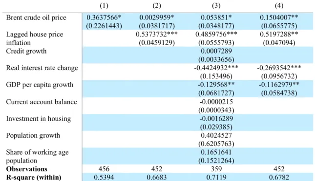
Now we can estimate the model specified by Equation 1 (see section 4.1) and the corresponding results are presented in Table 3. The first estimated values, presented in column 1 Table 3, comes from regressing Brent crude oil price on house price inflation. This partial regression model was constructed to include the isolated effect of unconditional within country correlation, doing so by specifying the model to include country and quarterly fixed effects. The relation between house price inflation and Brent crude oil price appears to be significantly positive and remains so even when adding another independent variable, the lag of the determinant (see column 2 Table 3). The lagged house price inflation variable suggests a strongly significant relationship with the dependent variable, as expected from the simple regression model presented previously. The third column of Table 3 accounts for all the chosen determinants of the model. Brent crude oil and the lagged house price inflation remains significantly positive related to the house price inflation. However, the magnitude of the Brent crude oil price coefficient is fluctuating depending on the other variables included in the model, whilst the lagged house price inflation is consistent throughout. For the other determinants of house price inflation, real interest rate change and GDP per capita growth is significant at a 5% level. Both variables appear to have a negative relationship with house price inflation. The

(26)

remaining variables does not seem to have a significant relationship with the dependent variable.1

Table 3. Results of Brent crude oil price, lagged house price inflation and other

determinants of the dependent variable.

(1) (2) (3) (4)

Brent crude oil price 0.3637566* (0.2261443) 0.0029959* (0.0381717) 0.053851* (0.0348177) 0.1504007** (0.0655775) Lagged house price

inflation 0.5373732*** (0.0459129) 0.4859756*** (0.0555793) 0.5197288** (0.047094)

Credit growth 0.0007289

(0.0033656)

Real interest rate change -0.4424932***

(0.153496) -0.2693542*** (0.0956732)

GDP per capita growth -0.129568**

(0.0681727)

-0.1162979** (0.0584738)

Current account balance -0.0000215

(0.0000343)

Investment in housing -0.0016289

(0.029385)

Population growth 0.4024527

(0.6205763) Share of working age

population

0.1651641 (0.1521264)

Observations 456 452 359 452

R-square (within) 0.5394 0.6683 0.7119 0.6782 The dependent variable is house price inflation. Country and year fixed effects are included in all specifications. Robust standard deviations in brackets. * (**) [***] stands for significance at the 10% (5%) [1%] level.

A last model estimate was made only including the significant variables from column 3. The new results are presented in column 4. When comparing the independent coefficient values with the previous one we can see that there are some differences. The R-square value seems to have dropped by a few decimal points and the overall model has a larger span of observations, meaning that the panel is more balanced than previously or due to the drop of variables. The Brent crude oil price coefficient appears to have increased by 0.1 compared to the previous model, that included all variables. However, the house price inflation lag is still the strongest indicator. A reason to why house price inflation is dependent on its own lag can be explained by it being based on its own historical data.

1_{New information regarding the trade status of Denmark have been brought} forward, that Denmark was in fact an oil exporter and not an oil importer as we expected it to be. Hence, a remake of the model has been made excluding Denmark from the sample. The results indicated no significant difference in the coefficient estimates and no change of the sign.

(27)

The results from this model can help to explain that there is a significant relationship between the oil price and the house price in our sampled countries, since the oil price have a significant impact on house price inflation. There is an issue regarding the sign of the relationship, as our model concludes that there is a positive relationship between the variables. This evidence contradicts a major share of previous research papers, which provide findings of a negative relationship between oil and house prices (see Bernanke, 2010; Kaufmann et al., 2011; Leamer, 2007; Hamilton, 2005). By directly comparing our linear regression model to the corresponding results from Breitenfellner et al. (2015), it is clear that we analyse opposite relationship signs. They receive a negative relationship between oil prices and house prices, however one similarity is identified. It regards the relatively small coefficient estimates of the energy price inflation, which indicates that even though there is a positive relationship between energy inflation and house price inflation it is rather small. The same observation goes for the estimated value of the oil price in our model, that the effect is small. Furthermore, other theoretical linkages suggesting a negative relationship have been made. The European Central Bank (2010), claim that increases in the oil price will affect house prices through a direct and indirect income and demand channel, causing house prices to fall.

On the contrary, empirical findings that support our result regarding a positive linkage between oil price and house price inflation are presented by Antonakakis et al. (2016) and Yiqi (2017). Antonakakis et al. (2016) finds that dynamic co-movements between the housing and oil markets are positive in some recessions in the U.S. during the 19th_century. While Yiqi (2017) concludes that there is a positive relationship between oil prices and house price inflation on the Norwegian market. There are also some theoretical linkages presented that support the suggested positive linkage. Regarding the construction and building operational costs, as the cost of the construction of residential buildings rise as a consequence of increasing oil prices, the result might cause the supply of houses to decrease. In turn, a decrease in supply causes upward pressure on the house prices. It can also be explained by changes in the financial markets. As rises in inflation expectations, a result of increasing oil prices, causes investors to become keener on investing in the oil and housing market as they serve as a hedge against inflation.

(28)

One might have expected the outcome to be different in regards to the previous research, when a lot of emphasis lays on explaining a negative relationship. However, as there is evidence for a positive relationship one might argue that the result is accurate. Possible reasons to why research papers have come to different conclusion could be due to different samples, inclusion of various time period etc. Another possible reason could regard the different geographic conditions of the samples.

Moving on to the estimate of real interest rate changes suggest a negative correlation to house price inflation. Theoretical research proves that this relationship is reliable, as the demand for housing can be explained by movements in the interest rate. The effect of an increase in mortgage interest rates causes the demand for housing to fall, as it gets more expensive to lend money which indirectly puts downward pressure on house prices. The relationship could also be explained by increasing mortgage delinquency rates, due to the consequence of an increased interest rate. Households do not afford to keep their homes and are forced to sell to a potential lower price than it’s worth due to a falling investment demand in housing.

When analysing the results of GDP per capita growth, one can see that the variable exhibit a significantly negative relationship to house price inflation. This is not to be expected from theory, however one could argue that house price inflation would be relying on previous values ranging back in time.

Continuously, one can see that no variables defined as demographic variables (share of working age population and population growth) is included in the chosen regression model. This could suggest that the demographic differences among the sampled countries do not have relevant effect on the overall house pricing. However, one could not fully exclude these variables from the analysis solely based on this research, since it could show an entirely different result if it were to be applied on countries that do not share the same economical and geographical similarities as with our sample used in this analysis. Concluding that, a large share of similarities rather than differences could be an indication to why these variables are insignificant. To identify the influence the demographic variables has on house pricing, an inclusion of more countries with geographic difference is recommended.

(29)

5.2 Result – Logit Model

We proceed the analysis by looking at the role of oil price on historical house price turning points. The results from the probability model developed in section 4.2, Equation 2, will be presented in this section.

The identified turning points are presented in Table 4, where each period is a turning point corresponding to a downward correction in house prices. This downward correction is defined as the observation corresponding to a peak, as well as the previous and following quarter. The largest number of turning points in house prices are detected during 1991-93 (Gulf war) and during the financial crisis of 2008. The graphs of estimated turning points of house price inflation can be found in the Appendix Figure A1.

Table 4. Identified turning points for house prices.

Denmark 1993 Q3 2007 Q1 2010 Q4 Finland 1993 Q4 2011 Q2 2000 Q2 2017 Q2 2008 Q1 Norway 1997 Q4 2013 Q2 2000 Q2 2015 Q3 2002 Q2 2017 Q1 2007 Q3 Sweden 1991 Q1 2010 Q4 2001 Q3 2016 Q1 2007 Q3 2017 Q3

The results taken from the misalignment estimate are measures of long-run elasticities for each individual country and their associated quarterly time-period. The data estimation of misalignment is presented in the Appendix (Table A2) for all sampled countries, separately.

We proceed the analysis by looking at the role of oil price on historical house price turning points. The probability model developed in Equation 3 has been tested. The results are presented in Table 5. In the first column of the table, a simple bivariate model is tested

(30)

between Brent crude oil price and the identified turning points of house prices. The result does not prove any significant relationship between the probability of oil price affecting the turning points in house prices. In the second column, the measure of misalignment is added to expand the model.

Table 5. Estimation results for conditional logit models of house price turning points.

(1) (2) (3) (4) (5) (6) (7)

Brent crude oil price 0.004359 (0.006405) 0.003827 (0.006923) -0.001468 (0.010151) 0.002454 (0.007016) -0.002354 (0.010645) -0.003346 (0.017452) Misalignment 0.655943 (1.095937) 0.839418 (1.307980) 0.509120 (1.753920) 1.766303 (1.864595) 2.110226 (3.372399) Credit growth 0.012499* (0.007593) 0.007044 (0.011138) 0.006845* (0.004227) Real interest rate

change 0.025643 (0.131966) 0.0184631 (0.216490) GDP per capita growth 0.496816** (0.258909) 0.344843 (0.278468) 0.372485* (0.232341) Current account balance -5.52E-05 (7.95E-05) -3.26E-05 (0.000130) Investment in housing 0.009691 (0.078674) -0.023866 (0.125314) Share of working age population -0.330499 (0.443785) -0.267578 (0.607171) Population growth 0.859150 (1.129676) 0.628992 (1.596557) Observations 459 398 391 395 331 327 429 R-square (McFadden) 0.002644 0.005341 0.046413 0.004277 0.013287 0.029143 0.028565

The dependent variable equals one in the identified turning point period and zero otherwise. Robust standard errors in brackets. * (**) [***] stands for significance at the 10% (5%) [1%] level.

Neither misalignment nor oil prices suggest any significant relationship to the probability of turning points occurring. In the following columns, an expanded range of determinants were added to account for the macroeconomic fundamentals, monetary policy and credit developments (column 3), the housing market variable (column 4) and the demographic variables (column 5). Throughout the different estimates, only column 3 showed signs of significance for two variables credit growth and GDP per capita growth. The last column accounts for the two identified significant variables, indicating that they have a positive relationship to the probability of the dependent variable taking the value of one. However, the coefficient estimates are relatively small.

(31)

The results of Table 5 contradict the hypothesised relationship between the turning points of house prices and the oil price, as it fails to provide a significant relationship of Brent crude oil. Comparable research by Breitenfellner et al. (2015) reached a positive significant relationship between energy price inflation and house price turning points. Possible reasons to why our estimated model fails to explain the correlation compared to Breitenfellner et al. (2015) could be due to various reasons; specification differences in the estimated data points of the turning points and misalignment, the use of Brent crude oil price as the main determinant instead of energy price inflation, the sampled countries and the included time span. Although oil prices serve as an explanatory variable and hence accounts for a large share of the overall energy price inflation, other variables explaining fluctuations in energy price are excluded. Combined with the fact that the comparable research covers a broader time span, where they include the 70s and 80s. One can suggest that not including data of previous decades may have changed the outcome. Assumptions are made that oil price had a greater impact on the house price inflation in the earlier decades, since households had a more oil intense consumption and are now shifting towards more renewable consumption patterns. It can also be explained by the fact that our sample size is much smaller in comparison and that it does not cover as much of the movement of the house and oil markets.

5.3 Results – Net Export vs Net Import

Providing answers to whether there is a significant difference between exporting and importing oil countries in terms of effects regarding the housing market can be explained by the results presented in Table 6. The result is estimated based on Equation 1, pooled for each country respectively (full results are presented in Appendix Table A8). The defined net export country in our case is Norway while the remaining three countries represents net import economies. The previous research of country specific effects in terms of trade (see Killins et al., 2017; Khiabani, 2015; Filis and Chatziantoniou, 2014), states that the housing market of exporting countries are more sensitive to changes in oil price. However, Killins et al. (2017) points out that even though demand shocks have a statistical effect on housing they are economically negligible.

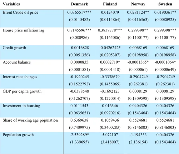
As one can see in Table 6, the estimated coefficients for the countries are significant at 10%, with exceptions for Finland. Evaluating the effect of Brent crude oil price our result

(32)

suggests that there is no substantial difference in the estimates. They are all reverting around a coefficient of 0.03-0.02. An interesting point is that Denmark shows the strongest relationship among the sample, even though it is an importing country. All in all, we cannot find evidence that differentiate export countries from import countries in terms of the oil price market affecting house price inflation. This contradicts the stated theoretical evidence presented, however one can point out once more that even if there would have been a significant difference between the trading status, it can be negligible.

Table 6. Oil price effects on house price inflation presented for each country separately.

Brent crude oil

Denmark 0.0365517*** (0.0115482) Finland 0.0124079 (0.0114864) Norway 0.0281124** (0.0116363) Sweden 0.0190361** (0.0080925)

The dependent variable is house price inflation. Robust standard deviations in brackets. * (**) [***] stands for significance at the 10% (5%) [1%] level.

(33)

6. Conclusion

Since the Great Financial Recession of 2007-09 and the burst of the house price bubble, economists have raised their awareness of the importance of understanding the causes and consequences of such crises. The house market inflation has been demonstrated to be affected by several different aspects of economy and geographical variables. The focus of the research questions in this paper have been laid on the role of oil prices as the main determinant of house price inflation in the sampled housing market.

The empirical analysis discusses the three different aspects; oil price on house price inflation, oil price on house price turning points and the differentiated trading patterns of oil in the countries. Concerning the first estimated model, the empirical results showed that there is a positive significant relationship between oil price and house price inflation, which can be explained by both previous research and theoretical linkages. In the second estimated model, we could not find a valid relationship between the main dependent variable and house price turning points. The only significant explanatory variables were real interest rate and GDP per capita. When considering the division of net import and net export trading behaviour of the sampled countries in terms of oil, no significant difference was found regarding the effect on their house price inflations.

The research question has been answered by the empirical analysis giving the answer that there is a positive relationship between oil price and house price inflation. This can be explained by the theoretical linkages suggesting that the relationship is positive, which are the construction and building operational costs and the financial market linkages, as they appeared to be the dominant ones. Where the cost of construction regarding residential buildings increases as an effect of rising oil prices, this causes the supply of houses to decrease and the price of houses to rise. In regard to the financial market, rises in inflation expectations causes investors to want to invest in the oil and housing market, since they serve as a hedge against inflation when oil prices rise. Moving forward, one should not exclude oil price as an independent variable explaining house price inflation as it has been proven to be significant empirically. However, one should be aware of the arguable differences of the impact oil prices have on house price inflation and also the extent of the effect.

(34)

As a suggestion, it would be interesting to better comprehend the impact of the geographical differences of the samples, both on national level but also to include regional aspects. In that way one could perhaps explain gain a greater insight to why oil prices may be positively related to house price inflation. We expect the regional aspect to shed light on the consumer behaviour and the demand for regional housing options in terms of urbanisation. One might find higher demand for housing in the city centre, together with a limited supply for residential and the restriction of not being able to construct more houses causes the price to increase. The upward pressure on the house prices in the city, can be further reinforced by people wanting to live close to their work (usually located in centre or close to the city). Since, an increase in oil price causes the transportation costs to rise, some might consider moving closer. Hence, the demand increases even more. The question of intense oil consumption patterns has been mentioned earlier in the paper, one would find it interesting to investigate that further. This could be done by having two separate time series, where one is identified as the highly dependent oil consumption period and the other one as the less dependent consumption period. This could incorporate the aspect of environment awareness, which is a well discussed topic in this modern society.

(35)

References

Antonakakis, N., Gupta, R., Muteba Mwamba, J.W., 2016. Dynamic comovements between housing and oil markets in the US over 1859 to 2013: a note. Atlantic Economic Journal 44, 377-386.

Bjørnland, H.C., Jacobsen, D.H., 2009. The role of house prices in the monetary policy transmission mechanism in small open economies. Working paper 2009/06, Norges Bank.

Breitenfellner, A., Cuaresma, J.C., Mayer, P., 2015. Energy inflation and house price corrections. Energy Economics 48, 109-116.

Bry, G., Boschan, C., 1971. Cyclical Analysis of Time Series: Selected Procedures and Computer Programs, NBER. Technical Working Paper No. 20.

Caballero, R., Fargi, E., Gourinchas, P., 2008. Financial crash, commodity prices and global imbalances. NBER Working Paper 14521.

Cramer, J.S., 1991. The LOGIT model for economists. Edward Arnold Publishers, London, 1991.

Crespo Cuaresma, J., 2010. Can emerging asset price bubbles be detected? OECD Economics Department Working Papers 772.

Dickey, D.A., Fuller, W.A., 1979. Distribution of the estimators for autoregressive time series with a unit root. Journal of the American Statistical Association 74(366), 427-431.

Edelstein, P., Kilian, L., 2009. How sensitive are consumer expenditure to retail energy prices? Journal of Monetary Economics 56, 766-779.

El-Gamal, M.A., Jaffe, A.M., 2010. Energy, financial contagion, and the dollar. Working paper, department of economics, Rice University and James A. Baker III Institute for Public Policy.

European Central Bank, 2010. Energy markets and the euro area marcoeconomy. Occasional paper series 113. European Central Bank.

Filis, G., Chatzaintoniou, I., 2014. Financial and monetary policy responses to oil price shocks: Evidence from oil-importing and oil-exporting countries. Review of

Quantitative Finance and Accounting, 42(4), 709-729.

Frankel, J.A., 2008. The effect of monetary policy on real commodity prices. In: Compbell, J. (Hg.) Asset prices and monetary policy. NBER, University of Chicago press.

(36)

Fuss, R., Zietz, J., 2016. The economic drivers of differences in house price inflation rates across MSAs. Journal of Housing Economics 31, 35-53.

Goodheart, C., Hofmann, B., 2008. House prices, money, credit and the macroeconomy. Oxford Review of Economic Policy 24, 180-250.

Gujarati, D.N., Porter, D.C., 2009. Basic Econometrics. (5. Ed.) Boston: McGrawHill. Hamilton, J., 2009. Causes and consequences of the oil shock of 2007-2008. Brooking Papers on Economic Activity.

Higgins, M., Klitgaard, T., Lerman, R., 2006. Recycling petrodollars. Current issues in economics and finance 12/09. Federal Reserve Bank of New York.

International Monetary Fund, 2008. The changing housing cycle and the implications for monetary policy. World Economic Outlook, pp. 103–132 (Washington, D.C., April) Jung, H., Park, C., 2011. Stock market reaction to oil price shocks: A comparison between an oil-exporting economy and an oil-importing economy. Journal of Economic Theory and Econometrics, 22(3), 1-29.

Kaufmann, R.K., Gonzales, N., Nickerson, T.A., Nesbit, T.S., 2011. Do household energy expenditures affect mortgage delinquency rates? Energy Economics. 33, 188-194.

Killins, R.N., Egly, P.V., Escobari, D., 2017. The impact of oil shocks on the housing market: Evidence from Canada and U.S. Journal of Economics and Business 93, 15-28. Leamer, E.E., 2007. Housing is the business cycle. NBER Working paper series 13428, September. National Bureau of Economic Research.

Mishkin, F.S. (2007). Housing and the monetary transmission mechanism. NBER Working Paper Series, 13518.

Quigley, J.M., 1984. The production of housing services and the derived demand for residential energy. The RAND Journal of Economics 15, 555.

White, H., 1980. A heteroscedasticity-consistent covariance matrix estimator and a direct test for heteroscedasticity. Econometrica 48, 817-838.

Yiqi, Y., 2017. The effect of oil prices on housing prices in the Norwegian market. Norwegian School of Economics, master thesis within economics.

(37)

Appendix

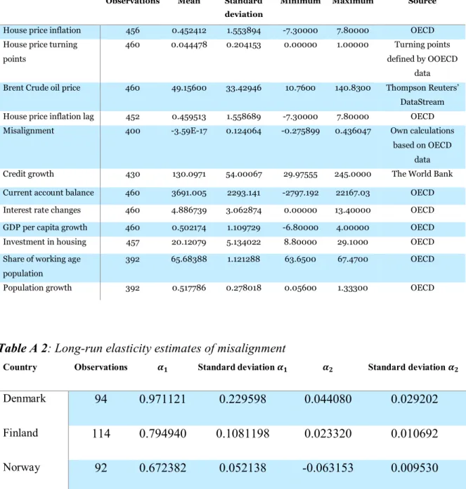
Table A 1: Descriptive statistics of the variables used in the empirical models.

Observations Mean Standard deviation

Minimum Maximum Source

House price inflation 456 0.452412 1.553894 -7.30000 7.80000 OECD House price turning

points

460 0.044478 0.204153 0.00000 1.00000 Turning points defined by OOECD

data Brent Crude oil price 460 49.15600 33.42946 10.7600 140.8300 Thompson Reuters’

DataStream House price inflation lag 452 0.459513 1.558689 -7.30000 7.80000 OECD Misalignment 400 -3.59E-17 0.124064 -0.275899 0.436047 Own calculations

based on OECD data Credit growth 430 130.0971 54.00067 29.97555 245.0000 The World Bank Current account balance 460 3691.005 2293.141 -2797.192 22167.03 OECD Interest rate changes 460 4.886739 3.062874 0.00000 13.40000 OECD GDP per capita growth 460 0.502174 1.109729 -6.80000 4.00000 OECD Investment in housing 457 20.12079 5.134022 8.80000 29.1000 OECD Share of working age

population

392 65.68388 1.121288 63.6500 67.4700 OECD Population growth 392 0.517786 0.278018 0.05600 1.33300 OECD

Table A 2: Long-run elasticity estimates of misalignment

Country Observations 𝜶𝟏 Standard deviation 𝜶𝟏 𝜶𝟐 Standard deviation 𝜶𝟐

Denmark 94 0.971121 0.229598 0.044080 0.029202

Finland 114 0.794940 0.1081198 0.023320 0.010692

Norway 92 0.672382 0.052138 -0.063153 0.009530

Sweden 100 1.391068 0.119953 -0.002715 0.012723

Dynamic OLS, with up to two lags and leads of first difference explanatory variables included in all regressions (Schwarz).