ANALYTICAL SOLUTIONS FOR MULTIPLE-MATRIX IN FRACTURED RESERVOIRS:
APPLICATION TO CONVENTIONAL AND UNCONVENTIONAL RESERVOIRSby
ii
A thesis submitted to the Faculty and the Board of Trustees of the Colorado School of Mines in partial fulfillment of the requirements for the degree of Master of Science (Petroleum Engineering).
Golden, Colorado Date ______________
Signed: ______________________ Mehmet Ali Torcuk
Signed: ______________________ Dr. Hossein Kazemi Thesis Advisor Golden, Colorado Date ______________ Signed:______________________ Dr. William Fleckenstein Professor and Head Department of Petroleum Engineering
iii ABSTRACT
In this thesis, I present a new method to model heterogeneity and flow channeling in petroleum reservoirs—specially reservoirs containing interconnected microfractures. The method is applicable both to conventional and unconventional reservoirs where the interconnected microfractures form the major flow path. The flow equations, which could include flow contributions from matrix blocks of various size, permeability and porosities, are solved by the Laplace transform analytical solutions and finite-difference numerical solutions. The accuracy of flow from and into nano-Darcy matrix blocks is of great interest to those dealing with unconventional reservoirs. Thus, matrix flow equations are solved using both pseudo-steady-state (PSS) and unpseudo-steady-state (USS) formulations.
The matrix blocks can be of different size and properties within the representative elementary volume (REV) in the analytical solutions and within each control volume (CV) in the numerical solutions. While the analytical solutions were developed for slightly compressible linear systems, the numerical solutions are general and can be used for non-linear multi-phase, multi-component flow problems.
The mathematical solutions were used to analyze the long-term performance of a gas well and two oil wells in two separate unconventional reservoirs. Finally, the formulations were used to assess enhanced oil recovery potential from a typical nano-Darcy matrix block. It is concluded that matrix contribution to flow is very slow in a typical low-permeability unconventional reservoir and much of the enhanced production is from the fluids contained in the microfractures than in the matrix.
In addition to field applications, the mathematical formulations and solution methods are
presented in a transparent fashion to allow easy utilization of the techniques for reservoir and engineering applications.
iv
TABLE OF CONTENTS
ABSTRACT ... iii
LIST OF FIGURES ... vi
LIST OF TABLES ... vii
ACKNOWLEDGEMENT ... viii
CHAPTER 1 INTRODUCTION ... 1
CHAPTER 2 SINGLE-MATRIX AND MULTIPLE-MATRIX MODELS ... 4
2.1 Homogeneous Single-Matrix Model ... 4
2.2 Multiple-Matrix Model ... 5
CHAPTER 3 MATRIX-FRACTURE TRANSFER FUNCTIONS ... 6
3.1 Pseudo-Steady State Transfer Functions ... 6
3.2 Unsteady State Transfer Functions ... 7
CHAPTER 4 LAPLACE DOMAIN ANALYTICAL SOLUTIONS FOR PSS AND USS TRANSFER FUNCTIONS ... 10
4.1 Laplace Domain Solutions for Pseudo-Steady State Transfer Functions ... 10
4.1.1 Solutions for Single-matrix Problem ... 10
4.1.2 Solutions for Multiple-matrix Problem ... 11
4.2 Laplace Domain Solutions for Unsteady State Transfer Functions ... 12
4.2.1 Solutions for Single-matrix Problem ... 12
4.2.2 Solutions for Multiple-matrix Problems ... 14
CHAPTER 5 EXTENSION OF SINGLE-PHASE THEORY TO WATER-OIL FLOW ... 18
CHAPTER 6 CLOSED FORM SOLUTIONS FOR PRESSURE TRANSIENT TEST ANALYSIS WITH USS TRANSFER FUNCTION ... 20
6.1 Closed-Form Solutions for Single-Matrix Model ... 20
6.1.1 Early Time Closed-Form Solution ... 21
6.1.2 Intermediate Time Closed-Form Solution ... 21
6.1.3 Late Time Closed-Form Solution ... 22
6.2 Closed-Form Solutions for Multiple-Matrix Model ... 24
5.2.1 Early Time Closed-Form Solution ... 25
6.2.2 Intermediate Time Closed-Form Solution ... 26
6.2.3 Late Time Closed-Form Solution ... 27
CHAPTER 7 PRESSURE DISTRIBUTION IN A NANO-DARCY MATRIX BLOCK ... 29
v
8.1 Example 1: Long-Term Production Data From a Horizontal Well in Bakken in Field 1 ... 32
8.2 Example 2: Long-Term Production Data From a Horizontal Well in Bakken in Field 2 ... 34
8.3 Example 3: Long-Term Shale Gas Production Data From a Horizontal Well in Field 3 ... 35
8.4 Example 4: Pressure Transient Test Example From a Horizontal Well in Bakken in Field 3 .... 36
CHAPTER 9 DISCUSSION, CONCLUSIONS AND RECOMMENDATIONS ... 39
LIST OF SYMBOLS ... 41
REFERENCES CITED ... 44
APPENDIX A DERIVATION OF UNSTEADY-STATE TRANSFER FUNCTIONS ... 46
APPENDIX B DERIVATION OF THE LAPLACE DOMAIN SOLUTIONS ... 51
B.1 Laplace Domain Solutions for Uniform Spherical Matrix Blocks ... 51
B.2 Laplace Domain Solutions for Non-Uniform Spherical Matrix Blocks ... 55
APPENDIX C DERIVATION OF NUMERICAL SOLUTION FOR MULTIPLE-MATRIX PSS MODEL ... 57
vi
LIST OF FIGURES
Figure 1.1: An outcrop of fractured basement rock from Alcova Reservoir, Wyoming (Courtesy: H.
Kazemi, CSM) ... 1
Figure 1.2: An idealized schematic of multi-stage hydraulic fracturing in unconventional reservoirs ... 2
Figure 2.1: Idealization of the heterogeneous dual-porosity medium with uniform cubic matrix blocks (Warren and Root, 1963) ... 4
Figure 2.2: Schematic of a fractured dual-porosity medium with non-uniform matrix blocks ... 5
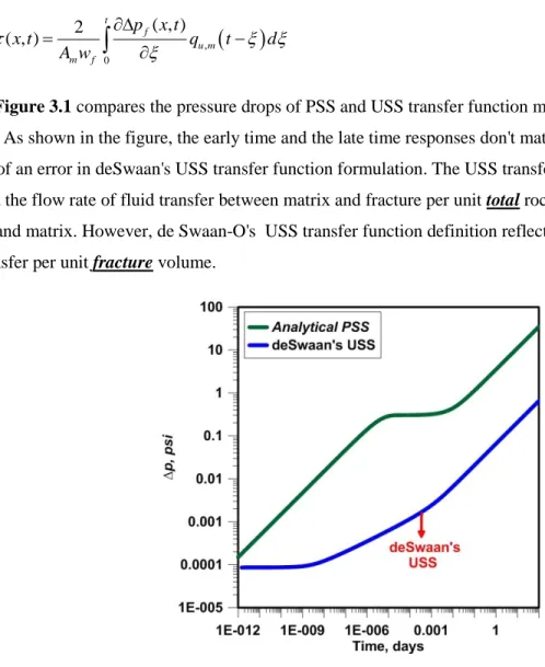
Figure 3.1: Comparison of pressure responses of PSS and de Swaan-O's USS models ... 7
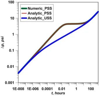
Figure 4.1: Comparison of dual-porosity model pressure responses ... 13
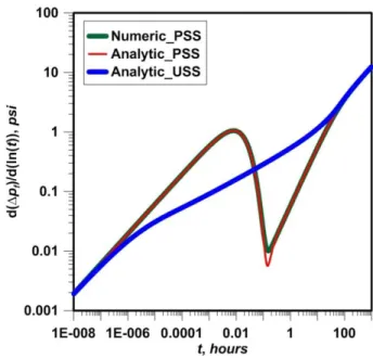
Figure 4.2: Comparison of dual-porosity model pressure-derivative responses ... 14
Figure 4.3: Pressure drops in fracture and each matrix block for triple-matrix Example 1 ... 16
Figure 4.4: Pressure drops in fracture and each matrix block for triple-matrix Example 2 ... 17
Figure 6.1: Pressure and logarithmic derivative of pressure for horizontal well example ... 24
Figure 6.2: Pressure drop as a function of t1/4 for bilinear flow analysis ... 28
Figure 7.1: Schematic of equal volume rings inside a spherical matrix block ... 29
Figure 7.2: Average pressure drop in the spherical matrix and the pressure drops in each region ... 31
Figure 8.1: Long term production data from a single-stage hydraulically fractured horizontal well in the Bakken in Field 1 ... 33
Figure 8.2: Long term production data from a 20-stage hydraulically fractured horizontal well in the Bakken in Field 2 ... 34
Figure 8.3: A typical long-term shale gas production data (Nobakht and Mattar, 2010) ... 36
Figure 8.4: Pressure and pressure derivative for field Example 4 ... 37
vii
LIST OF TABLES
Table 4.1 – Input data for triple-matrix example-1 ... 15
Table 4.2 – Input data for triple-matrix example-2 ... 16
Table 6.1 – Input data for Flow through a 5000-ft horizontal well ... 23
Table 7.1 – Input data for pressure distribution in a matrix block example ... 31
Table 8.1 – Data For Bakken Field Example-1... 33
Table 8.2 – Triple-Matrix Properties For Field Example-1 ... 33
Table 8.3 – Data For Bakken Field Example-2... 34
Table 8.4 – Triple-Matrix Properties For Field Example-2 ... 35
Table 8.5 – Data For Shale Gas Field Example ... 36
Table 8.6 – Data For Bilinear Flow Analysis ... 37
viii
ACKNOWLEDGEMENT
Firstly, I would like to thank my advisor, Dr. Hossein Kazemi, not only his contributions to this study but for the outstanding mentorship and guidance that he has provided me. His ideas opened up my horizon. I am thankful to members of dissertation committee: Dr. Azra Tutuncu, Dr. Yu-Shu Wu, and Dr. B. Todd Hoffman for their valuable comments on this study. I am also thankful to all professors in Petroleum Engineering Department at Colorado School of Mines, for their contributions to my academic background. Special thanks to Basak Kurtoglu for the valuable discussions, suggestions and comments she has provided me throughout the course of this thesis.
Financial assistance provided by Marathon Center of Excellence for Reservoir Studies (MCERS) is gratefully acknowledged.
During the course of this thesis, I have benefited from the kind assistance of many friends. First, I wish to express my sincere thanks to Denise Winn-Bower for her patience and helps. I am especially grateful to all my friends who are either in Turkey or in US. It is impossible to list all of your names here. I would like to thank them all for their enjoyable friendship.
Finally, but most deeply, I thank to my family and my girlfriend, Canan Aslan for the moral support that they have provided me.
This thesis is dedicated to my grandfather, Mehmet Ali Torcuk who had been a great source of inspiration.
1 CHAPTER 1 INTRODUCTION
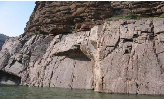
Fractures in a petroleum reservoir are created by natural forces, by man-made interventions, or combination of the two. The natural fractures are created by folding, faulting, and subsidence of geologic structures over a long period of time. The giant carbonate oilfields in the Middle East are good examples of naturally fractured reservoirs. Fig. 1.1 shows an outcrop of a fractured basement rock from Alcova reservoir in Wyoming overlain by Madison formation.
Figure 1.1: An outcrop of fractured basement rock from Alcova Reservoir, Wyoming (Courtesy: H. Kazemi, CSM)
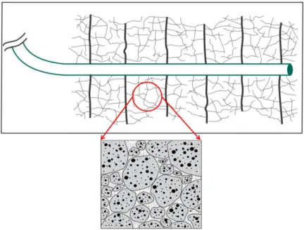
In addition to the natural fractures, engineering activities, such as water injection and hydraulic fracture stimulation also cause creation of fractures in a petroleum reservoir. In the last decade, there has been a great interest in enhanced oil and gas recovery in unconventional shale reservoirs. To make shale reservoirs productive, multistage hydraulic fracturing has been used to break the tight shale matrix into smaller pieces to create larger surface areas of contact (microfractures). Multistage hydraulic fracturing creates a dual-porosity environment in the vicinity of the hydraulic fracture. An idealized schematic of a multi-stage hydraulic fracturing in an unconventional reservoir is shown in Fig. 1.2. The near wellbore region includes a high density of microfractures which are created by stress changes resulting from hydraulic fracture stimulation.
2
Figure 1.2: An idealized schematic of multi-stage hydraulic fracturing in unconventional reservoirs Presence of fractures in petroleum reservoirs requires techniques to characterize flow in fractured reservoirs. Because of fractures' extreme heterogeneity and anisotropy, characterization of fractured reservoirs has been a challenging issue. For instance, fractures can negatively affect the success of an EOR project because of flow channeling of the injected fluids. On the other hand, primary production from unconventional reservoirs is enhanced because of the presence of fractures. Both in naturally fractured reservoirs and hydraulically fractured reservoirs, the matrix blocks are heterogeneous and have different sizes and shapes. To model fluid flow in a such fractured reservoir, the mathematical
formulations must account for heterogeneity of the matrix blocks.
Mathematical models describing the fluid flow in dual-porosity media began with papers from Barenblatt et al. (1960) and Warren-Root (1963). These models assume pseudo-steady state (PSS) fluid transfer from matrix to fracture. Later, a model, which considered unsteady-state (USS) or transient fluid transfer between matrix and fracture, was reported by Kazemi (1969) and de Swaan-O (1976). The Barenblatt and Warren-Root models ignore spatial distribution of pressure and transient flow in the matrix block. Each matrix block is assigned an average pressure; that is it is assumed that pressure is uniform in the matrix block.
In this work, I focus on the modeling of fluid flow in naturally fractured conventional and unconventional reservoirs. A multiple-matrix model is presented to account for the flow contributions of various matrix blocks having different geometric shapes and different properties. The most common flow hierarchy in a fractured petroleum reservoir is: matrix to fracture to wellbore (if it is a naturally fractured
3
reservoir) or matrix to natural fractures to hydraulic fracture to wellbore (if it is a hydraulically fractured reservoir). In this study, I consider the 1D flow from matrix to natural fractures to a hydraulic fracture which is also the wellbore. I mainly focus on the developments of analytical solutions for multiple-matrix model. However, the multiple-matrix model presented in this study can be used for 3D numerical modeling of single and multi-phase flow. Furthermore, it can also be used in compositional modeling of petroleum reservoirs to capture PVT phase behavior variability in the matrix blocks.
The organization of this thesis is as follows: First, I give the formulation for single phase flow in a dual-porosity reservoir supported by a uniform set of matrix blocks (single-matrix case). Then this formulation is extended to multiple-matrix model where a non-uniform set of matrix blocks support flow into the fractures. Next, I present the relevant pseudo-steady state and unsteady state transfer functions. Then, I develop the Laplace domain analytical solutions for both the single- and multiple-matrix models. In addition, I provide the closed form solutions for pressure transient test applications. The theoretical development is followed by examples to show applications to field problems. In these field problems, I show the effects of heterogeneity variation of matrix blocks on well performance. Finally, I present a discussion on the work done and give the conclusion of the work.
4 CHAPTER 2
SINGLE-MATRIX AND MULTIPLE-MATRIX MODELS
The concept of dual-porosity modeling includes a continuum of interconnected fractures and a set of matrix blocks (cubes, spheres and slabs) imbedded in the fractures. However, in nature, the matrix block size and properties vary; which is the focus of this thesis. In this chapter, I first give the diffusivity equation for 1D fluid flow in dual-porosity reservoirs. Next, I present the basic definitions and equations used in the multiple-matrix model.
2.1 Homogeneous Single-Matrix Model
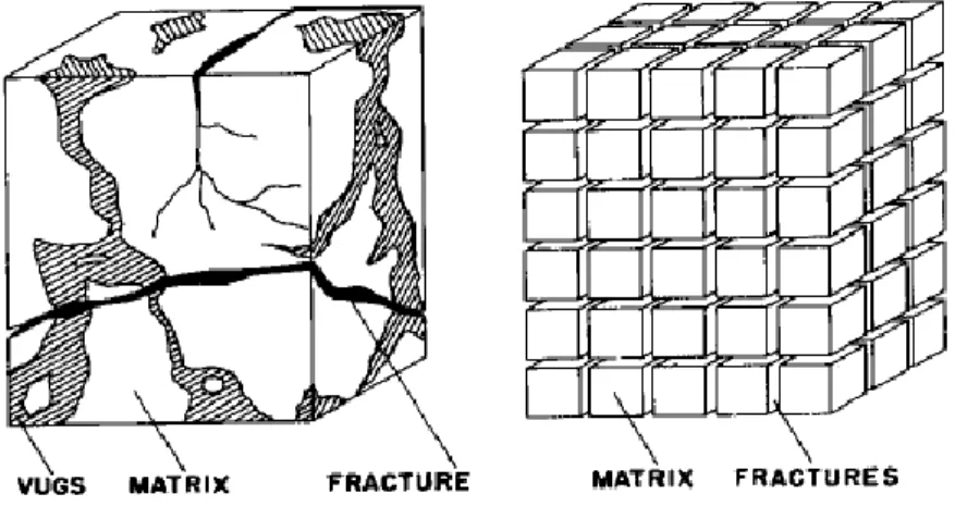
Naturally fractured dual-porosity reservoirs are usually idealized as a set of uniform matrix blocks with the geometric shapes of cube, sphere and slab (Fig. 2.1).
Figure 2.1: Idealization of the heterogeneous dual-porosity medium with uniform cubic matrix blocks (Warren and Root, 1963)
To couple the fluid flow between the matrix and the fracture with uniform matrix block
idealization of fractured reservoirs, a transfer function is added to the continuity equation. The continuity equation for the single phase, slightly compressible, 1D flow in a dual-porosity media with uniform size, homogeneous and isotropic matrix is given by:
2 , 2 ( , ) ( , ) 0.006328kf eff pf x t ct f pf x t x t [2.1] Where:5 f i wf
p p p
[2.2]
2.2 Multiple-Matrix Model
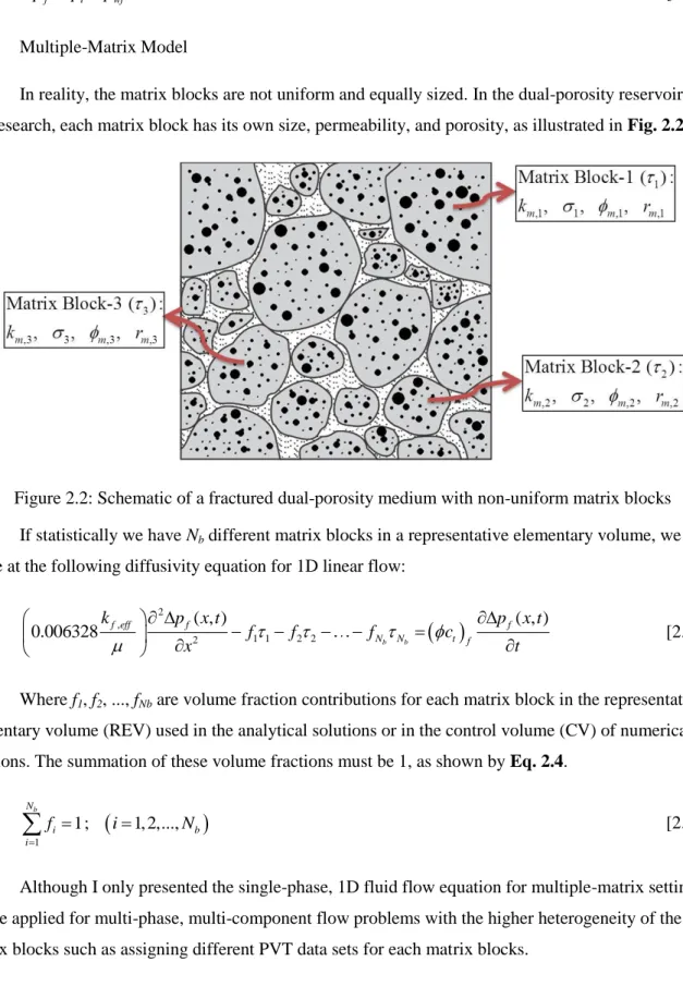
In reality, the matrix blocks are not uniform and equally sized. In the dual-porosity reservoir of this research, each matrix block has its own size, permeability, and porosity, as illustrated in Fig. 2.2:
Figure 2.2: Schematic of a fractured dual-porosity medium with non-uniform matrix blocks If statistically we have Nb different matrix blocks in a representative elementary volume, we
arrive at the following diffusivity equation for 1D linear flow:
2 , 1 1 2 2 2 ( , ) ( , ) 0.006328 b b f eff f f N N t f k p x t p x t f f f c x t [2.3]Where f1, f2, ..., fNb are volume fraction contributions for each matrix block in the representative
elementary volume (REV) used in the analytical solutions or in the control volume (CV) of numerical solutions. The summation of these volume fractions must be 1, as shown by Eq. 2.4.
1 1; 1, 2,..., b N i b i f i N
[2.4]Although I only presented the single-phase, 1D fluid flow equation for multiple-matrix setting, it can be applied for multi-phase, multi-component flow problems with the higher heterogeneity of the matrix blocks such as assigning different PVT data sets for each matrix blocks.
6 CHAPTER 3
MATRIX-FRACTURE TRANSFER FUNCTIONS
In this chapter, I present the pseudo-steady state and unsteady state matrix-fracture transfer functions for both uniform matrix blocks and the matrix blocks having different geometric shapes and properties. I start with the derivation of pseudo-steady state transfer function for single phase flow. Then, I present the unsteady-state transfer functions for sphere, slab and cuboid matrix blocks. Here I show the basic steps of the derivation, however, full derivation of unsteady-state transfer functions can be found in Appendix A. The transfer functions presented in this chapter are going to be used in both the analytical and numerical solutions in the next chapters.
3.1 Pseudo-Steady State Transfer Functions
The dual porosity diffusivity equation considers the conservation of mass in the fracture. The transfer function in Eq. 2.1, reflects the volume of fluid transferred from matrix to the fracture per unit rock volume per unit time. If I consider the conservation of mass principle in the matrix system, I can write:
m t m p c t [3.1]The relationship between the conservation of mass principle and fluid flow between matrix and fracture can be obtained from the Darcy's law. The transfer function representing the fluid transfer between fracture and the surrounding rock matrix for single-phase flow is:
m f m k p p [3.2]If we combine Eqs. 3.1 and 3.2, we get:
m m f m t m k p p p c t [3.3]Where the shape factor, , for a cuboid matrix block with dimensions Lx, Ly and Lz is:
2 2 2 1 1 1 4 x y z L L L [3.4]
7
The definition of the pseudo-steady state transfer function is independent from the shape of the matrix blocks, however, the shape factor has different definitions for the matrix blocks having different geometry.
3.2 Unsteady State Transfer Functions
As stated before, the fluid transfer from shale matrix blocks to the fractures takes a long time to reach pseudo-steady state regime because of the extremely tight nature of the matrix blocks. Thus, I first focused on formulating the transfer function to model the transient fluid flow between fracture and matrix. My derivation of unsteady state (USS) transfer functions, for different geometric shapes, followed the formulation provided by de Swaan-O in 1976 (shown below):
, 0 ( , ) 2 ( , ) t f u m m f p x t x t q t d A w
[3.5]Figure 3.1 compares the pressure drops of PSS and USS transfer function models for an example
problem. As shown in the figure, the early time and the late time responses don't match each other. This is because of an error in deSwaan's USS transfer function formulation. The USS transfer function must represent the flow rate of fluid transfer between matrix and fracture per unit total rock volume containing fracture and matrix. However, de Swaan-O's USS transfer function definition reflects the flow rate of fluid transfer per unit fracture volume.
8
The new unsteady-state (USS) transfer function, which represents the flow rate of fluid transfer between fracture and matrix per unit rock volume, is given below:
, 0 ( , ) 1 ( , ) t f u m m p x t x t q t d V
[3.6]Where, qu m, is the flow rate caused by a unit pressure drop at the matrix surface. For a spherical matrix, qu m, is given by the following equation:
, , ; ( , ) 0.006328 m m m u m m r r p r t x k q x t A r [3.7]I begin to illustrate the use of Eq. 3.6 by assuming that the matrix blocks are spheres and
surrounded by fractures. The pressure change at any point, r, in such a sphere, when the surface pressure m
p is suddenly decreased by 1 unit of pressure, is given below (adopted from the heat conduction
problem by Carslaw and Jaeger, 1959):
22 2 1 1 2 1 , ; 1 exp sin n m m m n m m r n t n r p r t x r n r r
[3.8] Where:
0.006328 m m t m k c [3.9] o m m m p p p [3.10]
1 m m p r r psi [3.11]Thus, for the spherical matrix block, the transient transfer function becomes:
2
2 1 0 , 6 ( , ) 0.006328 exp t f m m n p x t k x t n t d
[3.12]Where is the shape factor for a spherical matrix block as shown: 2 2 m r [3.13]
9
I also consider slab and cuboid (cuboid means rectangular cuboid in this thesis) for the shape of the matrix blocks and present the unsteady-state transfer functions for these shapes (for derivations see Appendix A). For a slab matrix block, the transfer function is:
2
2 0 0 , 8 ( , ) 0.006328 exp 2 1 t f m m n p x t k x t n t d
[3.14]Where is the shape factor for a slab matrix block, given below: 2 2 z L [3.15]
And for a cuboid matrix block the transfer function takes the following form:
2 2 2 2 2 2 2 2 2 2 0 0 0 6 2 2 2 2 2 2 2 2 1 2 1 2 1 2 1 2 1 2 1 , 512 ( , ) 0.006328 2 1 2 1 exp 2 1 x y z l m n f m x m y z l L m L n L l m n p x t k x t l L m L n L
0 t d t
[3.16]Where is the shape factor for a cuboid matrix block:
2 2 2 2 1 1 1 x y z L L L [3.17]
10 CHAPTER 4
LAPLACE DOMAIN ANALYTICAL SOLUTIONS FOR PSS AND USS TRANSFER FUNCTIONS In this chapter, I present the Laplace domain analytical solutions for constant terminal rate and constant terminal pressure, both for single and multiple matrices using both the pseudo-steady state and unsteady state transfer functions. I evaluated these solutions in the Laplace domain and then numerically inverted the results into real time domain using numerical inverse of the Laplace transform (Stehfest, 1970).
4.1 Laplace Domain Solutions for Pseudo-Steady State Transfer Functions
I first present the analytical solutions for pseudo-steady state fluid transfer model. To develop the solutions, I used the transfer function presented in Section 3.1.
4.1.1 Solutions for Single-matrix Problem
The diffusivity equation for single-phase, slightly compressible, linear flow in a dual-porosity medium with uniform matrix block distribution is:
2 , 2 ( , ) ( , ) 0.006328 f eff f t f f k p x t p x t c x t [4.1]Where the transfer function is:
pf pm
[4.2] And
1
m f m D p p p t [4.3]Here, is inter porosity flow parameter and is fracture storativity ratio. The mathematical definitions of and are:
2 , m f eff k L k [4.4]
t f t f t m c c c [4.5]11 The dimensionless form of the diffusivity equation is:
2 2 Df Df Df Dm D D p p p p x t [4.6] Where: D x x W [4.7]
, 2 0.006328 f eff D t f t m k t t c c L [4.8]
,
141.2 f eff o Df D f f k h p t p p t qB [4.9]Taking the Laplace transform of Eqs. 4.3 and 4.6, and combining them, I have:
2 2 ( ) ( ) 0 Df D Df D D d p x g s p x dx [4.10]And the g(s) function is:
1
1 s g s s s [4.11]The wellbore pressure solution for this 1D, single-phase flow problem is:
2 Df p s s g s [4.12]4.1.2 Solutions for Multiple-matrix Problem
The pseudo steady state transfer function representing the flow rate of fluid transfer from each matrix block in a multiple-matrix model is:
, , ; 1, 2,..., m i i i f m i b k p p i N [4.13]12 And
, , , , ; 1, 2,..., m i m i i f m i t m i b k p p p c i N t [4.14]The wellbore pressure solution in the Laplace domain for this problem is as single-matrix solution, as shown below:
2 Df p s s g s [4.15]However, the g(s) function has a modified form to capture the flow contributions from non-uniform matrix blocks, Eq. 4.16:
1
2
1 2 1 2 1 1 1 ... 1 1 1 b b b N N N s s s g s s f f f s s s [4.16]4.2 Laplace Domain Solutions for Unsteady State Transfer Functions
This section presents the Laplace domain analytical solutions for unsteady state transfer functions presented from Eq. 3.11 to 3.15. I developed the solutions for only spherical matrix blocks, however, similar solutions can be derived for cuboid and slab matrix blocks by following the similar procedures. 4.2.1 Solutions for Single-matrix Problem
The 1D dual-porosity pressure solution at the any point x, for constant terminal rate, in the Laplace domain, is (for full derivation, see appendix B):
,
1 , exp 0.006328 f f eff qB p x s g s x k hL s g s [4.17]And for x=0, the pressure solution at the wellbore intersected by an axial vertical fracture is:
, 1 0, 0.006328 f f eff qB p s k hL s g s [4.18]13
2 2 1 , , 6 1 0.006328 t f m n f eff f eff m c k g s s k k s n
[4.19]Similarly, flow rate vs. time solutions for the constant terminal pressure case can be obtained. For instance the bottom-hole flow rate solution in the Laplace-domain is:
, 0 0.006328kf eff f x g s qB hL p s [4.20]After inverting Eq. 4.18 for the USS fluid transfer model, I compared the results with the numerical and analytical pseudo-steady-state (PSS) dual-porosity models. For analytical PSS model, I used the Laplace domain solution and calculated the pressure response in the Laplace domain. Then, I used numerical Laplace inversion to get the real time domain solutions. The numerical PSS results were generated by using the finite-difference numerical solution method. Fig. 4.1 is a comparison of the USS analytical pressure solution with the numerical and analytical PSS pressure solutions. The USS dual-porosity model presented in this thesis generates the same pressure drops as the analytical and numerical PSS dual-porosity models for early and late time periods. The solution difference in the intermediate times is because of the difference in the formulation of USS and PSS models. I emphasize that the USS formulation is physically a more realistic model.
14
Fig. 4.2 presents a comparison of pressure derivative for USS and PSS models. Both the
analytical and numerical steady state (PSS) models show the V-shape characteristic of pseudo-steady state model. However, the unpseudo-steady-state model doesn't have the V-shape character.
The pressure transient studies presented in this thesis indicate that the classical pseudo-steady-state (PSS) V-shape characteristic of the pressure derivative plot for dual-porosity reservoirs is unrealistic, especially for unconventional reservoirs.
Figure 4.2: Comparison of dual-porosity model pressure-derivative responses
4.2.2 Solutions for Multiple-matrix Problems
The analytical solutions of the dual-porosity problems are based on the assumption that the matrix blocks are uniform throughout the reservoir. However, in this thesis, I deal with non-uniformity and heterogeneity of matrix blocks. In my formulation, the Laplace domain analytical solutions for the multiple-matrix model are same as the solutions for the uniform matrix block case but the g(s) function is different.
15
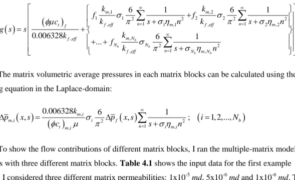
,1 ,2 1 1 2 2 2 2 2 2 1 1 , 1 ,1 , 2 ,2 , , 2 2 1 , , 6 1 6 1 0.006328 6 1 ... b b b b b m m n n f eff m f eff m t f m N f eff N N n f eff N m N k k f f k s n k s n c g s s k k f k s n
[4.21]The matrix volumetric average pressures in each matrix blocks can be calculated using the following equation in the Laplace-domain:
,
, 2 2 1 , , 0.006328 6 1 , m i , ; 1, 2,..., m i i f b n t m i i m i k p x s p x s i N c s n
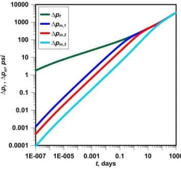
[4.22]To show the flow contributions of different matrix blocks, I ran the multiple-matrix model for two cases with three different matrix blocks. Table 4.1 shows the input data for the first example problem. I considered three different matrix permeabilities: 1x10⁻⁵ md, 5x10⁻⁶ md and 1x10⁻⁶ md. The matrix blocks were spheres and the radii were also different: 0.5 ft, 1.0 ft and 5.0 ft. The volume fractions were 0.10, 0.10 and 0.80. Fig. 4.3 shows the pressure drops in the fracture and each matrix block. The time required for matrix block-1 to reach the pseudo-steady state regime is about 0.4 day, while for second and third matrix blocks is 2 and 100 days, respectively. This clearly shows that increasing matrix block size and decreasing matrix permeability decreases the matrix contribution to flow.
TABLE 4.1 – INPUT DATA FOR TRIPLE-MATRIX EXAMPLE-1
Reservoir, Well, Fluid Properties Matrix Block-1 Matrix Block-2 Matrix Block-3
μ (cp) 0.02 km (md) 1x10 -5 5x10⁻⁶ 1x10⁻⁶ B (RCF/SCF) 1 φm 0.15 0.20 0.10 ct,m (1/psi) 1.5x10 -4 σ (1/ft2) 39.47 9.87 0.395 ct,f (1/psi) 5x10 -4 rm (ft) 0.5 1 5 h (ft) 30 f (fraction) 0.1 0.1 0.8 L (ft) 5000 φf 3.94x10 -5 k f,eff (md) 8.3x10 -4 q (SCF/D) 1000
16
Figure 4.3: Pressure drops in fracture and each matrix block for triple-matrix Example 1
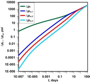
In the second example (Table 4.2), I used a fixed matrix porosity, 0.10, to see the effects of matrix size and permeability on the pressure drop in each matrix block. In this example, the matrix blocks were again spheres and the radii were 1.0 ft, 3.0 ft and 5.0 ft. I used the same matrix permeabilities: 1x10⁻⁵
md, 5x10⁻⁶ md and 1x10⁻⁶ md. The volume fraction of the first matrix block is 0.8, and the second and third matrix blocks have 0.1 for volume fractions.
TABLE 4.2 – INPUT DATA FOR TRIPLE-MATRIX EXAMPLE-2
Reservoir, Well, Fluid Properties Matrix Block-1 Matrix Block-2 Matrix Block-3
μ (cp) 0.02 km (md) 1x10⁻⁵ 5x10⁻⁶ 1x10⁻⁶ B (RCF/SCF) 1 φm 0.10 0.10 0.10 ct,m (1/psi) 1.5x10⁻⁴ σ (1/ft2) 9.87 1.096 0.395 ct,f (1/psi) 5x10 -4 rm (ft) 1 3 5 h (ft) 30 f (fraction) 0.8 0.1 0.1 L (ft) 5000 φf 2x10 -4 k f,eff (md) 8.3x10 -4 q (SCF/D) 1000
Fig. 4.4 shows the resulting pressure drops in the fracture and in each matrix block. Similar to the
17
longer time to reach the pseudo-steady state flow regime. This clearly indicates that the property of one matrix block in a multiple-matrix system affects the pressure responses of other matrix blocks.
18 CHAPTER 5
EXTENSION OF SINGLE-PHASE THEORY TO WATER-OIL FLOW
The equations for the multi-phase, multi-component flow problems are highly non-linear, thus the analytical solutions for these non-linear systems are not present. However, for an approximation, I show the application of multiple-matrix model to the Buckley-Leverett (B-L) displacement, a quasi-linear form of multi-phase flow in dual-porosity reservoirs. The linearized B-L displacement in the fracture for a dual-porosity system with unsteady state transfer function was first presented by de Swaan-O (1978):
, , , wf wf t f f S x t S x t u x t [5.1]Here is the unsteady state (USS) transfer function for water entering the matrix (or, equivalently, oil leaving the matrix):
0 , t wf t S x t R e d
[5.2]Laboratory experiments indicate that, the cumulative oil recovery by water imbibition and/or gravity drainage from matrix can be approximated by the following exponential curve (Kazemi, et al., 1992):
1 t
RR e [5.3]
Where, R is the maximum oil volume recovered per unit rock volume at infinite time and R is
the oil volume recovered per unit rock volume at any time t. The exponential decline parameter,, can be calculated by matching experimental data using Eq. 1.3. The calculated exponential decline parameter includes the combined effects of viscous, capillary and gravity forces for the specific rock sample. The Laplace domain solution of the water saturation at any point (x, t) in the fracture space for a single-matrix is:
, 1 1 , exp 1 wf t f f R s S x s x s u s [5.4]If we have multiple-matrices in each representative elementary volume (REV), the water-oil displacement equation, Eq. 5.1, becomes:
19
1 2
, 1 2 , , ... b b N wf wf t f N f f f S x t S x t u f f f x t [5.5]The unsteady-state transfer function for each matrix block is:
, 0 , ; 1, 2,..., i t wf t i i i b S x t R e d i N
[5.6]In this multiple-matrix setting, each matrix block may have its own mass transfer coefficient (i) and ultimate recovery per unit rock volume (R,i). The water saturation in the fracture for multiple-matrix model in the Laplace-domain is:
1 ,1 2 ,2 1 2 1 2 , , 1 1 ... 1 , exp 1 1 b b b b f f wf t f N N N f N R R f f s s s S x s x s u R f s [5.7]20 CHAPTER 6
CLOSED FORM SOLUTIONS FOR PRESSURE TRANSIENT TEST ANALYSIS WITH USS TRANSFER FUNCTION
To derive the closed form solutions for both single- and multiple-matrix model for interpretation of the pressure transient test data, I present the formulation in terms of dimensionless parameters. The dimensionless diffusivity equation in the Laplace-domain is:
2 2 Df Df D p g s p x [6.1]6.1 Closed-Form Solutions for Single-Matrix Model
The diffusivity equation for single phase, slightly compressible linear fluid flow in a dual porosity medium with uniform matrix block distribution is:
, 2
2 0.006328 kf eff pf ct f pf x t [6.2]I need to define the dimensionless parameters to write the diffusivity equation (Eq 6.2) in dimensionless form: D x x L [6.3]
, 2 0.006328 f eff D t f t m k t t c c L [6.4]
,
141.2 f eff Df D f k h p t p t qB [6.5]By using these dimensionless variables, I obtain the dimensionless diffusivity equation as following (for full derivation, see Appendix B):
2 2 2 1 3 1 3 coth Df Df D p s sp x s s [6.6] Where:21
2 1 3 1 3 coth g s s s s s [6.7]The wellbore pressure solution in the Laplace domain for this problem is given as following:
2 Df p s s g s [6.8]6.1.1 Early Time Closed-Form Solution
In early times, because the time is very small, the Laplace transform variable s becomes very large. Thus the g(s) function reduces to:
g s s [6.9]
The wellbore pressure solution in the Laplace domain becomes:
3 22 Df p s s [6.10]Inverting into the real time domain, I obtain:
4Df D
p t t
[6.11]
In dimensional form, the early time pressure solution for a two-sided reservoir model is:
1 2 , 8.128 1 f t f eff f qB p t t c k hL [6.12]Please note that, in the above solution, the flow rate is in STB/D and the time is in hours. 6.1.2 Intermediate Time Closed-Form Solution
The intermediate time flow regime follows the early time fracture flow and matrix starts to feed the reservoir in this flow period. Thus, to obtain the closed-form solution for intermediate flow regime, fracture storativity can be ignored. For intermediate times, g(s) function can be approximated (for x>3.6, coth(x)≈1) :
22
3
1
g s s s [6.13]The wellbore pressure solution in the Laplace domain becomes:
5 4 2 3 1 Df p s s [6.14]Inverting into the real time domain yields:
1 4 2 5 3 1 4 D Df D t p t [6.15]Under this assumption, I arrive at the closed-form pressure solution for intermediate-time (the flow rate is in STB/D and the time is in hour):
1 4 1 4 , 63.82 1 f m t f eff m qB p t t k c k hL [6.16]And the effective permeability can be estimated from the slope of pf
t vs t1 4 plot, as following:
1 2 2 , intermediate 63.82 1 f eff m t m qB k m hL k c [6.17]6.1.3 Late Time Closed-Form Solution
In the late times, the reservoir acts like a single-porosity media. Thus, for late times, the g(s) function can be used as:
g s s [6.18]
The wellbore pressure solution in the Laplace domain becomes:
3 2 2 Df p s s [6.19]23
The real time domain inversion of the wellbore pressure solution is:
4Df D D
p t t [6.20]
The closed-form solution for late time flow regime becomes:
1 2 , 8.128 1 f t f eff f m qB p t t c k hL [6.21]The slope of pf
t vs t1 2 plot can be used to estimate the effective permeability from linear flow period:
2 , 8.128 1 f eff linear t f m qB k m hL c [6.22]As an example, Fig. 6.1 shows the single-matrix USS pressure and pressure derivative (logarithmic derivative) profiles for flow through a 5000-ft horizontal well in a naturally fractured reservoir. The data used for the example problem are given in Table 6.1. Looking at the transition zone between the two linear flow periods, one can observe the absence of the V-shape feature of the classical pseudo-steady-state, dual-porosity model. The lack of such a V-shape feature is supported by field observations.
TABLE 6.1 – INPUT DATA FOR FLOW THROUGH A 5000-FT HORIZONTAL WELL
Reservoir, Well, Fluid Properties
μ (cp) 0.02 km (md) 1x10⁻⁵ B (RB/STB) 1 kf,eff (md) 2.8x10⁻⁴ ct,m (1/psi) 5x10 -4 σ (1/ft2) 4.1 ct,f (1/psi) 1.5x10 -4 rm (ft) 1.55 h (ft) 100 φf 2x10 -3 L (ft) 5000 φm 0.05 q (STB/D) 356.2
24
Figure 6.1: Pressure and logarithmic derivative of pressure for horizontal well example
I estimated the effective permebilities as 2.34x10⁻⁴ md and 2.82x10⁻⁴ md from the intermediate and late time flow solutions (Eqs. 6.17 and 6.22), respectively.
6.2 Closed-Form Solutions for Multiple-Matrix Model
The diffusivity equation for single phase, slightly compressible linear fluid flow in a dual porosity medium with non-uniform matrix block distribution is:
, 2
1 1 2 2 2 0.006328 kf eff pf f f ct f pf x t [6.23]And the unsteady-state transfer functions are for each matrix block are:
, , , 0 ( , ) 1 ( , ) ; 1, 2,..., t f i u m i b m i p x t x t q t d i N V
[6.24]The new definitions of dimensionless variables for MM setting are:
, 2 1 ,1 2 ,2 , 0.006328 ... b b f eff D t f t m t m N t m N k t t c f c f c f c L [6.25]25
1
,1 2
,2 ... b
, b t f t f t m t m N t m N c c f c f c f c [6.26]
, 2 , ; 1, 2,..., m i i i b f eff k L i N k [6.27]By using these dimensionless variables, I obtain the dimensionless diffusivity equation for multiple-matrix model as following (for full derivation, see Appendix B):
1 1 1 1 1 ,1 2 2 2 2 2 2 ,2 2 , 3 1 coth 3 1 coth 3 1 coth b b b b b b m Df m D N N N N N m N f s F s F r s f s p F s F r s x f s F s F r s Df sp [6.28] Where:
,
; 1, 2,..., t f i b t m i c F i N c
[6.29] 1 1 1 1 1 ,1 2 2 2 2 2 ,2 , 3 1 coth 3 1 coth ( ) 3 1 coth b b b b b b m m N N N N N m N f s F s F r s f s F s F r s g s s f s F s F r s [6.30]5.2.1 Early Time Closed-Form Solution
Because the early time flow is dominated by the fracture flow, I have the same early time solution with the single-matrix setting. The early time wellbore pressure solution is:
26
1 2 , 8.128 1 f t f eff f qB p t t c k hL [6.31]6.2.2 Intermediate Time Closed-Form Solution
Similarly to the single-matrix solution, for intermediate times, the g(s) function can be approximated as: 1 1 1 2 2 2 3 3 ( ) 3 b b b N N N f F s f F s g s s f F s [6.32]
The wellbore pressure solution in the Laplace domain becomes:
5 4 1 2 1 2 1 1 2 2 2 3 3 3 ... b b b b Df N N N N p s s f f f F F F [6.33]Inverting into real time domain gives:
1 4 1 2 1 2 1 1 2 2 2 5 3 3 3 4 ... b b b b D Df D N N N N t p t f f f F F F [6.34]And the closed-form pressure solution for intermediate-time in multiple-matrix setting is:
1 2 1 4 2 2 , 1 1 ,1 2 2 ,2 ,1 ,2 2 , , 63.82 1 ... b b b b f f eff m t m t m m N N m N t m N qB p t t k hL f k c f k c f k c [6.35]27
And the effective permeability for the multiple-matrix setting can be estimated from the slope of
fp t
vs t1 4 plot, as shown in the following equation:
2 , 2 2 1 1 ,1 ,1 2 2 ,2 ,2 2 , , 63.82 1 ... b b b b f eff bilinear m t m t m m N N m N t m N qB k m hL f k c f k c f k c [6.36]6.2.3 Late Time Closed-Form Solution
For multiple-matrix setting, I have the same late time approximation with single matrix setting, as shown by the following equation:
g s s [6.37]
And the wellbore pressure solution in the real time domain is:
4Df D D
p t t [6.38]
Because the definition of dimensionless time is different, I have a slightly different late time closed-form solution for multiple-matrix setting:
1 2 , 1 ,1 2 ,2 , 8.128 1 ... b b f f eff t f t m t m N t m N qB p t t k hL c f c f c f c [6.39]The slope of pf
t vs t1 2 plot can be used to estimate the effective permeability from linear flow period:
2 , 1 ,1 2 ,2 , 8.128 1 ... b b f eff linear t t t N t f m m m N qB k m hL c f c f c f c [6.40]I used the data set in Table 4.1 to generate the synthetic data for the triple-matrix example and then I plot pf
t vs t1 4 for the bilinear flow regime period (Fig. 6.2), I calculated the effective permeability as 7.77x10⁻⁴ md which originally was 8.3x10⁻⁴ md.28
29 CHAPTER 7
PRESSURE DISTRIBUTION IN A NANO-DARCY MATRIX BLOCK
The pressure distribution inside each matrix block can also be estimated by using the MINC (Multiple Interacting Continua) approach (Pruess and Narasimham, 1985). To estimate the pressure distribution, I divide the spherical matrix block into 3 segments having same volumes as shown in Fig.
7.1:
Figure 7.1: Schematic of equal volume rings inside a spherical matrix block
When I write the mass conservation equation between the transfer function and the three rings, I have three equations with three unknowns which are the pressure drops in each segment.
2 ,1 ,2
,1 3 ,1 , 2 1 0.006328 m4 m m m m t m m m p p p k r V c V r t [7.1]
,2 ,3 2 5 , 2 2 ,2 ,2 ,1 ,2 2 3 , 2 1 0.006328 4 0.006328 4 m m m m m t m m m m m m p p k r r p c V p p t k r r [7.2]
2 ,2 ,3
,3 5 ,3 , 2 2 0.006328 m4 m m m t m m m p p p k r c V r t [7.3]Taking the Laplace transform of mass conservation equations, respectively, yields:
2 ,1 ,2
3 ,1 ,1 , 2 1 0.006328 m4 m m m t m m m m p p k r V c V s p r [7.4]30
,2 ,3 2 5 , 2 2 ,2 ,2 ,1 ,2 2 3 , 2 1 0.006328 4 0.006328 4 m m m m t m m m m m m m p p k r r c V s p p p k r r [7.5]
2 ,2 ,3
5 ,3 ,3 , 2 2 0.006328 m4 m m t m m m m p p k r c V s p r [7.6]To solve the above equation set, I form the following matrix-vector system:
2 2 3 , 2 3 , 2 1 1 ,1 2 3 , 2 1 2 2 3 5 , 2 , 2 1 2 ,2 4 4 0.006328 0.006328 0 4 0.006328 4 4 4 0.006328 0.006328 0.006328 m m m m t m m m m m m m m m m t m m k r k r r r s c V k r r k r k r k r r r s c V
2 ,1 5 , 2 ,2 2 ,3 2 2 ,5 2 5 , 2 2 2 ,3 0 0 4 4 0.006328 0 0.006328 m m m m m m m m t m m p V p r p k r k r r r s c V [7.7] These matrix-vector system can be solved in the Laplace domain to get the pressure drops. A theoretical example case is presented below. The matrix blocks in this example were equally sized spheres. Fig. 7.2 shows the average pressure drop in the spherical matrix block and the pressure drops in each region. The data used to construct Fig. 7.2 are tabulated below.31
TABLE 7.1 – INPUT DATA FOR PRESSURE DISTRIBUTION IN A MATRIX BLOCK EXAMPLE
Reservoir, Well, Fluid Properties
μ (cp) 0.02 φm 0.15 B (RCF/SCF) 1 σ (1/ft2) 39.47 ct,m (1/psi) 1.5x10 -4 rm (ft) 0.5 ct,f (1/psi) 5x10 -4 f 0.1 h (ft) 30 φf 3.94x10 -5 L (ft) 5000 rm,1 (ft) 0.5 q (SCF/D) 1000 rm,2 (ft) 0.437 km (md) 1x10 -5 rm,3 (ft) 0.347
Figure 7.2: Average pressure drop in the spherical matrix and the pressure drops in each region
As shown in Fig. 7.2, the pressure drop in region 1, which is the outer and thinner region, follows the average pressure drop profile of whole matrix block. However, the second and third regions require longer times to follow the same line. For example, it requires about 30 days for the third region to reach the matrix average pressure drop.
32 CHAPTER 8 FIELD APPLICATIONS
In addition to the theoretical examples, in this thesis, I analyzed four field examples from unconventional reservoirs. These four field examples include three long-term production data from one gas and two separate oil wells, and a pressure build-up example from an oil well. The flowing pressure histories for the oil wells were estimated from surface pressure measurements.
8.1 Example 1: Long-Term Production Data From a Horizontal Well in Bakken in Field 1 The first example is a 8794-ft horizontal well in the Middle Bakken formation with open hole completion and single-stage hydraulic fracture in Field 1. The well has been producing for four years. To analyze the long-term production data, I used rate normalized pressure (p qo ) vs square-root of time (t1/2) plot. The linear flow equation for uniform matrix blocks (Eq. 6.21) can be written in the following form:
1 2 , 8.128 24 1 f t f eff f m p t B t q k hL c [8.1]And the effective permeability is:
2 , 8.128 24 f eff linear t f m B k m hL c [8.2]Fig. 8.1 shows the rate normalized pressure data as a function of square-root of time. It is clear
that linear flow regime dominates the long term production from the horizontal well in Field 1. The fluid properties are estimated from the PVT analysis and given in Table 8.1. I used the typical values of the matrix and fracture compressibilities in Bakken formation. Firstly, we analyzed the linear flow period by assuming the matrix blocks are uniform. Then, we extended our analysis for a triple-matrix example to show the effect of heterogeneity of matrix blocks on the effective permeability estimation.
Production data analyses show that a typical horizontal well in Bakken has an effective producing length which is about 20% of the total length (Kurtoglu, et al., 2012a). Thus, I used the effective
producing length as 1760 ft to estimate the effective permeability. From the linear flow analysis for uniform matrix blocks, the effective permeability was estimated as 3.66x10⁻² md. This calculated