Identiﬁcation of Stochastic Nonlinear Dynamical Models Using Estimating Functions

(1)

Identification of Stochastic Nonlinear Dynamical

Models Using Estimating Functions

MOHAMED RASHEED-HILMY ABDALMOATY

Doctoral Thesis

Stockholm, Sweden

(2)

TRITA-EECS-AVL-2019:63 ISBN 978-91-7873-267-8

Skolan för elektroteknik och datavetenskap Avdelningen för reglerteknik 100 44 Stockholm, Sverige Akademisk avhandling som med tillst˚and av Kungliga Tekniska högskolan framlägges till offentlig granskning för avläggande av teknologie doktorsexamen i elektro- och systemteknik fredagen den 6 september 2019 klockan 10.00 i sal F3, KTH Kungliga Tekniska högskolan, Lindstedtvägen 26, Stockholm.

(3)

Abstract

Data-driven modeling of stochastic nonlinear systems is recognized as a very challenging problem, even when reduced to a parameter estimation problem. A main difficulty is the intractability of the likelihood function which renders favored esti-mation methods, such as the maximum likelihood method, analytically intractable. During the last decade, several numerical methods have been developed to approxi-mately solve the maximum likelihood problem. A class of algorithms that attracted considerable attention is based on sequential Monte Carlo algorithms (also known as particle filters/smoothers) and particle Markov chain Monte Carlo algorithms. These algorithms were able to obtain impressive results on several challenging benchmark problems; however, their application is so far limited to cases where fundamental limitations, such as the sample impoverishment and path degeneracy problems, can be avoided.

This thesis introduces relatively simple alternative parameter estimation methods that may be used for fairly general stochastic nonlinear dynamical models. They are based on one-step-ahead predictors that are linear in the observed outputs and do not require the computations of the likelihood function. Therefore, the resulting estimators are relatively easy to compute and may be highly competitive in this regard: they are in fact defined by analytically tractable objective functions in several relevant cases. In cases where the predictors are analytically intractable due to the complexity of the model, it is possible to resort to plain Monte Carlo approximations. Under certain assumptions on the data and some conditions on the model, the convergence and consistency of the estimators can be established. Several numerical simulation examples and a recent real-data benchmark problem demonstrate a good performance of the proposed method, in several cases that are considered challenging, with a considerable reduction in computational time in comparison with state-of-the-art sequential Monte Carlo implementations of the ML estimator.

Moreover, we provide some insight into the asymptotic properties of the proposed methods. We show that the accuracy of the estimators depends on the model parameterization and the shape of the unknown distribution of the outputs (via the third and fourth moments). In particular, it is shown that when the model is non-Gaussian, a prediction error method based on the Gaussian assumption is not necessarily more accurate than one based on an optimally weighted parameter-independent quadratic norm. Therefore, it is generally not obvious which method should be used. This result comes in contrast to a current belief in some of the literature on the subject.

Furthermore, we introduce the estimating functions approach, which was mainly developed in the statistics literature, as a generalization of the maximum likelihood and prediction error methods. We show how it may be used to systematically define optimal estimators, within a predefined class, using only a partial specification of the probabilistic model. Unless the model is Gaussian, this leads to estimators that are asymptotically uniformly more accurate than linear prediction error methods

(4)

methods.

Finally, we consider the problem of closed-loop identification when the system is stochastic and nonlinear. A couple of scenarios given by the assumptions on the disturbances, the measurement noise and the knowledge of the feedback mechanism are considered. They include a challenging case where the feedback mechanism is completely unknown to the user. Our methods can be regarded as generalizations of some classical closed-loop identification approaches for the linear time-invariant case. We provide an asymptotic analysis of the methods, and demonstrate their properties in a simulation example.

(5)

Sammanfattning

Det är välkänt att datadriven modellering av icke-linjära stokastiska system är ett utmanande problem, även i fallen där det kan reduceras till ren parameterskat-tning. Den huvudsakliga sv˚arigheten är att likelihoodfunktionen inte är analytiskt hanterbar, vilket medför problem vid tillämpning av standardmetoder s˚asom maxi-mum likelihood. Under det senaste decenniet har numeriska algoritmer baserade p˚a sekventiell Monte Carlo (partikelfilter) rönt stort intresse. Dessa algoritmer har imponerande prestanda p˚a en rad benchmarkproblem; dock s˚a är deras praktiska tillämpning än s˚a länge begränsad till specialfall där fundamentala begränsningar kan undvikas.

Den här avhandlingen introducerar nya metoder som kan användas för parame-terestimering i en stor klass av icke-linjära stokastiska system. Metoderna baseras p˚a enstegsprediktorer som är linjära i systemets observerade utsignal. V˚ara nya metoder kräver inte att likelihoodfunktionen beräknas; istället använder de, i en rad relevanta fall, analytiskt hanterbara uttryck som gör dem högst attraktiva. I fallen där prediktorerna är analytiskt ohanterbara (p˚a grund av modellens komplexitet) kan man använda vanliga Monte Carlo-approximationer. Vi visar att klassiska resultat fr˚an asymptotisk teori kan användas under rimliga antaganden, och via dessa, att v˚ara föreslagna skattare är konsistenta samt asymptotiskt normalfördelade. Skattarnas prestanda utvärderas i numeriska simulationer, samt nyligen föreslagna benchmarkproblem baserade p˚a verklig data, med bra resultat.

Vidare diskuterar vi de föreslagna metodernas asymptotiska egenskaper: deras nogrannhet beror inte enbart p˚a hur modellen har parametriserats, utan även p˚a datans sannolikhetsdistribution (via dess tredje och fjärde ordningens moment). Speciellt visar vi att när modellen inte uppfyller antaganden om normalfördel-ning, s˚a är en prediktionsfelsmetod baserad p˚a ett normalfördelningsantagande inte nödvändigtvis bättre än en prediktionsfelsmetod baserad p˚a en viktad parameter-oberonde kvadratisk norm. V˚ar slutsats är att det därför inte är uppenbart vilken prediktionsfelsmetod som bör användas. Detta resultat st˚ar i kontrast mot den vedertagna uppfattningen som finns i delar av litteraturen.

Avhandlingen introducerar även den s˚a kallade skattningsfunktionsmetoden (främst utvecklad inom statistiklitteraturen) som en generalisering av maximum likelihood- och prediktionsfelsmetoderna. Vi visar hur denna metod kan användas för att systematiskt konstruera optimala skattare, inom en specifierad modellklass, fr˚an enbart partiella specifikationer p˚a den underliggande probabilistiska modellen. Detta ger skattare som asymptotiskt är likformigt mer noggrannare än linjära prediktionsfelsmetoder baserade p˚a kvadratiska optimeringsobjektiv. Vi härleder konvergensresultat, s˚asom konsistens, för dessa skattare under standardantaganden.

Slutligen behandlar vi identifieringsproblemet för ˚aterkopplade system som är stokastiska och icke-linjära. Vi behandlar ett par varianter p˚a antaganden om mät-samt processbrus, och p˚a kunskap om hur systemets ˚aterkoppling sker. Ett speciellt utmanande fall är när ˚aterkopplingsmekanismen är helt okänd. Metoderna vi föresl˚ar kan ses som generaliseringar av klassiska metoder för identifiering av ˚aterkopplade

(6)

(7)

،سراف �یل .أ ةیلاغلا ي�أ

ي�ح دیشر .د.أ بيب�ا ي �يأ

(8)

(9)

Acknowledgements

First and foremost, I would like to express my sincere gratitude to my supervisor H˚akan Hjalmarsson. I will forever be thankful to him for giving me the chance of pursuing a PhD degree, and for offering me his guidance, support, and patience throughout the years. His intuition and insight have always been invaluable, and I am truly grateful for the comments and feedback he provided until the last minute. Thank you H˚akan!

I am also grateful to Cristian Rojas, my co-supervisor, for generously sharing his vast knowledge and for his continuous help and advice, particularly in my first years as a PhD student.

My thanks also go to all my current and former colleagues in the division of Decision and Control Systems at KTH. In particular, I would like to thank my colleagues in the System Identification group: Robert Mattila, Matiás Müller, Rodrigo González, Mina Ferizbegovic, Ines Louren¸co, Diogo Rodrigues, Niklas Everitt, Cristian Larsson, Patricio Valenzuela, Afrooz Ebadat, Miguel Garlinho, Riccardo Sven Risuleo, and Giulio Bottegal, for the stimulating work environment and friendly companionship. Special thanks to Robert for translating the thesis abstract to Swedish. I would also like to thank Arda Aytekin, Valerio Turri, Pedro Pereira, Jezdimir Milosevic, Hamid Feyzmahdavian, Mohamed Sadegh and Takashi Tanaka for the good times, lunch breaks and conversations we had. Special thanks to Arda for sharing his IT knowledge with me. I am thankful to the administrators Felicia Gustafsson, Anneli Ström, Silvia Svensson, and Karin Karlsson Eklund for being very helpful and efficient at all times.

Lastly, I would like to thank my friends and family for their moral support, love, and encouragement. I thank my good friends Amin Hasan, Ahmed Nagm-Eldeen, and Mohamed Khalid for being there for me. I am thankful to Florence and St´ephane for always cheering for me. Thanks should also go to my sister Nisreen and my brother Ahmed for their love and for always believing in me. I am grateful to Eug´enie for her love, unwavering help and encouragement throughout the years. Finally, I am indebted to my parents, Laila Fares and Rasheed-Hilmy Abdalmoaty, for their unconditional love, care, and support, without which none of this would have been possible.

Mohamed Rasheed-Hilmy Abdalmoaty

August 2019 Stockholm, Sweden

(10)

(11)

Notations

A bold font is used to denote random variables and a regular font is used to denote realizations thereof. The symbol is used to terminate proofs.

Number Sets

N, N0 the set of natural numbers, N∶= {1, 2, . . . }, N0∶= N ∪ {0}.

Z the set of integers, Z∶= {0, ±1, ±2, . . . }.

R, R+ the sets of real numbers and nonnegative real numbers respectively.

Rd the Euclidean real space of dimension d∈ N.

Parameters and Constants

θ the parameter: a finite dimensional vector in Rdθ to be estimated.

θ○ the (assumed) true parameter.

Θ a compact subset of Rdθ.

{gk}∞k=1 impulse response sequence of a plant model.

{hk}∞k=0 impulse response sequence of a noise model.

dw, du, dy, dx the dimension of the process disturbance, the input signal, the

output signal, and the state process respectively; all in N.

Signals and Stochastic Processes

ζ= {ζ_t}t∈Z a generic vector-valued discrete-time stochastic process.

x= {xt}t∈Z a latent/state process.

u= {ut}t∈Z the input signal.

y= {yt}t∈Z the output signal.

w= {wt}t∈Z the process disturbance.

v= {vt}t∈Z the measurement noise (when it is white).

e= {et}t∈Z the prediction error process.

ε= {εt}t∈Z the (linear) innovation process.

Φζ(ω) the power spectrum of a process ζ, in which ω∈ R.

(16)

Vectors and Matrices

A(θ), B(θ), C(θ) deterministic matrices parameterized by θ. Z a column vector, Z∶= [ζ⊺₁, . . . , ζ⊺_N]⊺.

X a column vector stacking state vectors, X∶= [x⊺₀, . . . , x⊺_N]⊺. Ut a column vector stacking input vectors, U∶= [u⊺1, . . . , u⊺t]⊺.

Yt a column vector stacking output vectors, Yt∶= [y⊺1, . . . , y⊺t]⊺.

U, Y denote UN, YN respectively.

W a column vector stacking disturbance vectors, W ∶= [w⊺₁, . . . , w⊺_N]⊺. V a column vector stacking measurement noise vectors,

V ∶= [v⊺₁, . . . , v⊺_N]⊺.

E a column vector stacking prediction error vectors, E∶= [e⊺₁, . . . , e⊺_N]⊺. E a column vector stacking innovation vectors, E∶= [ε⊺

1, . . . , ε⊺N]⊺.

ˆ

y_t_∣t−1(θ) a parameterized one-step-ahead predictor of y.

̂

Y a column vector stacking one-step-ahead predictors of yt,

̂

Y ∶= [ˆy⊺₁_∣0, . . . , ˆy⊺_N_∣N−1]⊺.

ˆθ an estimate of θ or an estimator function (when it has an argument).

Functions and Operators

(⋅)−1 _{the inverse (of an operator or a square matrix).}

(⋅)⊺ _{the transpose (of a vector or a matrix).}

F⊺(θ), Σ−1(θ) means [F(θ)]⊺,[Σ(θ)]−1respectively.

vech[⋅] half-vectorization operator; for a symmetric matrix M of size n, vech[M] is the column vector of size n(n + 1)/2 obtained by

vectorizing the lower triangular part of M.

∥⋅∥2, ∥⋅∥Q the Euclidean norm and a weighted Euclidean norm. For any

vector x∈ Rn_{, n}_{∈ N and any positive definite matrix Q,}

∥x∥Q∶=√x⊺Qx.

q the shift operator on sequence spaces, q xt∶= xt+1 .

q−1 the backward shift operator on sequence spaces, q−1xt∶= xt−1.

G(q, θ) transfer operator plant model parameterized by θ. H(q, θ) transfer operator noise model parameterized by θ. f, gand h static (measurable) functions between Euclidean spaces. ψ one-step-ahead predictor function defining ˆy_t_∣t−1. ` scalar function used in the definition of prediction error

(17)

Notations xvii

Probability Spaces

(Ω, F, Pθ) generic underlying measure space. The measure is

parameterized by θ.

δx˜({x}) Empirical density function: δx˜({x}) ∶= 1 if x = ˜x, otherwise

δx˜({x}) ∶= 0.

E[⋅; θ] mathematical expectation with respect to Pθ.

E○[⋅] mathematical expectation with respect to the true underlying

measure of the data P○. If there exists θ○∈ Θ, E○[⋅] = E[⋅; θ○]

Eζ[⋅; θ] mathematical expectation with respect to the distribution of a

random vector ζ. The distribution is parameterized by θ.

p(ζ; θ) probability density function of a real random vector ζ

parameterized by θ with respect to the Lebesgue measure.

pζ(ζ; θ) the value p(ζ = ζ; θ).

p(ζ; θ) the likelihood function of θ given a realization of ζ.

p(ζ∣η; θ) conditional probability density function, parameterized by θ, of

a real vector-valued random variable ζ given a realization of another random variable η; that is p(ζ∣η = η; θ). The reference measure is always the Lebesgue measure.

ζ∣η a (conditional) random variable ζ with a PDF p(ζ∣η; θ).

E[⋅∣η; θ] conditional expectation given that η= η.

cov(ζ1, ζ2; θ) the covariance matrix of two random vectors ζ1, ζ2; that is

E[(ζ1− E[ζ1; θ])(ζ2− E[ζ2; θ])⊺; θ].

var(ζ; θ) the variance of a real-valued random variable ζ.

↝ means “converges in distribution to”.

a.s.

Ð→ means “converges almost surely to”.

ˆ

θ estimator of θ; that is ˆθ∶= ˆθ(DN).

Function Spaces

L2(Ω, F, Pθ) the Hilbert space of real-valued random variables with finite

second moments. Generally, the arguments will be dropped and only L2 will be used.

Ln₂(Ω, F, Pθ) the Hilbert space of random variables in Rn with entries in

L2, and n∈ N. Generally, the arguments will be dropped and

only Ln

2 will be used.

ϕ a generic (measurable) test function. sp{S} the linear span of the subset S⊂ L2.

PS[⋅] the orthogonal projection operator of L2or Ln2 onto a closed

(18)

Data Sets

N the cardinality of the data set, N∈ N.

Dt a set of input and output pairs, Dt∶= {(yk, uk) ∶ 1 ≤ k ≤ t}, t ≤ N.

Distributions

N (µ(θ), Σ(θ)) the multivariate Gaussian distribution with a mean vector

µ(θ) and a covariance matrix Σ(θ); parameterized by θ.

U ([a, b]) the uniform distribution over the closed interval[a, b].

Other

0,∞ the zero vector and infinity respectively.

M the number of samples/particles in a Monte Carlo method.

∶ means “such that”.

∀ means “for all”.

∼ means “is distributed according to”; It is used in conjunction with probability measures, distribution functions or PDFs.

i.i.d.

∼ means “is independently and identically distributed according to”.

∝ means “is proportional to”.

∶= means “is defined as”.

≈ means “is approximately equal to”.

d

= means “equal in distribution to”.

1 a column vector of ones with the appropriate dimension. I the identity matrix with the appropriate dimension.

t discrete-time index for signals and time-dependent functions. z complex variable of the z-transform.

ω angular frequency variable, or a weight in an importance

sampling method. arg min

θ∈Θf(θ) the set of global minimizers of a real-valued function f over a

compact set Θ. sol

θ∈Θ{f(θ) = 0} the set of solutions to the algebraic problem f(θ) = 0 over Θ.

log(⋅) the natural logarithm function, log∶ R+/{0} → R.

O(N) a function such that∣O(N)∣≤ CN with finite C ∈ R+, N ∈ N.

V2 for any vector V ∶= [v1. . . vN]⊺ we define V2∶= [v12. . . v 2 N]⊺.

(19)

Notations xix

Σ1⪰ Σ2, Σ1≻ Σ2 for any two symmetric matrices Σ1and Σ2, of the same size,

means that the matrix Σ∶= Σ1− Σ2is a positive semidefinite

matrix or a positive definite matrix respectively.

[V ]i,[M]ij for a vector V , the symbol [V ]i denotes the ith entry of V ;

similarly, for a matrix M, the symbol[M]ij denotes the

ijth _{entry of M.}

∂θf(θ) gradient of a real-valued function f: a row vector with

entries[∂θf(θ)]i∶= ∂θif(θ) ∶=

∂

∂θif(θ) where θi∶= [θ]i.

∂_θ2f(θ) Hessian of a real-valued function f: a square matrix with

entries[∂2

θf(θ)]ij∶= ∂θijf(θ) ∶=

∂2

∂θi∂θjf(θ) where θi∶= [θ]i.

∂θV(θ) for a dθ-dimensional vector θ, and an n-dimensional vector

function V(θ), denotes an n × dθ matrix with entries

(20)

(21)

Abbreviations

i.i.d. Independent and Identically Distributed.

CRLB Cram´er-Rao Lower Bound.

EF(s) Estimating Function(s).

EnKF Ensemble Kalman Filter.

KF Kalman Filter.

LTI Linear Time-Invariant.

MC Monte Carlo.

MCMC Markov Chain Monte Carlo.

ML Maximum Likelihood.

MLE Maximum Likelihood Estimate/Estimator.

MSE Mean-Square Error.

MMSE Minimum MSE.

OE-predictor Output-Error predictor. OE-QPEM OE-predictor Quadratic PEM.

OE-WQPEM OE-predictor Weighted Quadratic PEM.

OL-predictor the linear (in y) MMSE one-step-ahead predictor. OL-QPEM OL-predictor Quadratic PEM.

OL-GPEM Prediction Error Method based on the optimal linear predictor and a “Gaussian log-likelihood form” criterion.

PDF Probability Density Function.

PE Prediction Error.

PEM(s) Prediction Error Method(s).

SMC Sequential Monte Carlo.

SOE-QPEM Simulated OE-QPEM.

SOL-QPEM Simulated OL-QPEM. SOL-GPEM Simulated OL-GPEM.

(22)

(23)

Chapter 1

Introduction

In this chapter, we introduce the topic of the thesis and motivate the considered problem. The first two sections have appeared previously in [3]. The last section gives an outline of the thesis content and highlights its main contributions.

1.1 Data-Driven Learning of Dynamical Models

System identification is a scientific method concerned with dynamical models learning based on observed data (see [114, 153, 179, 215, 232]). It can be described as the joint activity of dynamical systems modeling and parameter estimation. Like any other scientific method, system identification is used to acquire new knowledge, or correct and improve existing knowledge based on measurable evidence. In system identification, the evidence is given in terms of a set of measured signals (variables) known as the data set. The mathematical model used to describe the relation between the measured signals constitutes the hypothesis of the method.

In engineering sciences, system identification is used as a tool for the design or the operation of engineering systems. For example, most of the modern automatic control techniques and signal processing and fault detection methods are based on mathematical models obtained using system identification techniques.

1.1.1 Systems

The term “system” refers to any spatially and temporally bounded physical or conceptual object within which several variables interact to produce an observable phenomena (see [119, 156, 254]). The observable variables are called the outputs (or the output signals) of the system. We will assume here that the outputs reflect the behavior of the system in response to some external stimuli. The external variables that can be altered by an extraneous observer are called the inputs (or the input signals) of the system. All external variables that cannot be altered by the observer are called disturbances (or disturbance signals). In some but not all cases, the disturbances can be directly observed (measured).

(24)

It is assumed here that a system follows some sort of causality. The inputs and the disturbances are considered to be the causes, and the outputs are the observable effect. This definition of a system is quite general and can accommodate many observable phenomena. For example, a system can be a human cell, an electric motor, an aircraft, an economic system, or the solar system. It is possible to define inputs, disturbances and outputs for each of these systems. For instance, the solar system is affected by the gravity of neighboring stars, which cannot be altered by the observer; such gravitational effect is therefore a disturbance. On the other hand, the behavior of an aircraft is influenced by the engine thrust which can be taken as an input, but also by gust which is a disturbance. For more complex systems, the discrimination between inputs, disturbances, and outputs becomes less clear.

In many scientific fields, including engineering sciences, most of the systems are dynamical systems with some sort of memory. The outputs of a dynamical system at a certain time do not only depend on the inputs and disturbances at the same time, but also on their histories.

1.1.2 Mathematical Models

A fundamental step of any system identification procedure is the specification of a mathematical model set. A mathematical model is an abstract representation of a system in terms of a mathematical relation between its inputs, outputs and disturbances. In practice, a mathematical model is seen as an approximation of the real-life system’s behavior, and cannot provide an exact description; consequently, one system can have several models under several assumptions and/or intended uses.

Dynamical systems are usually modeled by a set of (partial or ordinary) differen-tial or difference equations. Models corresponding to differendifferen-tial equations are called continuous-time models, while those corresponding to difference equations are called discrete-time models. When the coefficients of these equations are independent of time, the models are called time-invariant models.

A generic causal discrete-time model can be defined by the equation

yt= ft({uk}tk=−∞,{ζk}tk=−∞; θt)

in which t∈ Z is an integer representing time, yt∈ Rdy is a real vector representing

the value of the output at time t, the sequence{uk}tk=−∞represents the input history

up to time t, in which ut∈ Rdu is a real vector representing the value of the input

at time t, and the sequence{ζk}tk=−∞ represents the history of the disturbances

up to time t where ζtis a real vector representing the values of the disturbances.

The symbol ftdenotes a generic mathematical function modeling the cause/effect

relationship between the inputs and disturbances and the outputs. The function is parameterized by a parameter θtthat is usually a finite-dimensional real vector,

θt∈ Rdθ for all t∈ Z and some constant dθ∈ N, in which case the model is said to be

parametric. The subscript t indicates that the function and the parameter may, in general, vary with time.

(25)

1.1. Data-Driven Learning of Dynamical Models 3

A model may be derived using physical laws and prior knowledge about the system. However, in cases where physical modeling is not possible due to the complexity of the system, standard classes of models can be used. An important subset of models is the set of parametric linear time-invariant models. These are models that assume a linear relationship between the inputs, the disturbances and the outputs such that the parameter is time-independent: θt= θ for all t ∈ Z

(see Section 2.1.3). Linear models are used extensively in practice, even when the underlying system exhibits a nonlinear behavior. This is mainly due to the fact that the estimation and feedback control theory is well-developed and well-understood for linear models (see [9, 10, 94, 117, 118, 186, 212, 255]). However, when linear models are not accurate enough for the intended use, nonlinear models have to be considered (see [204] for a related discussion).

1.1.3 Estimation Methods

Once a model set has been determined, the next step of the system identification procedure is to choose a parameter estimation method. The choice is guided by the available assumptions on the data and the model class. The main goal of the estimation method is the evaluation of the unknown parameter vector θ. An estimate is usually computed, based on a set of recorded input and output signals over a finite time interval, by solving either an optimization problem or an algebraic problem. Furthermore, the estimation method must provide some kind of accuracy measure for the computed estimate.

Since the values of the disturbances are usually unknown, an uncertainty concept must be introduced. There are two main approaches for the characterization of uncertainty: the unknown but bounded approach, and the stochastic approach. In the unknown but bounded approach (see [163]), the uncertainty is characterized by defining a membership set for all uncertain quantities. That is, for all t∈ Z, the values assumed by ζtbelong to some known bounded set. Based on this constraint

and the given data, a set of feasible parameters can be determined and a parameter can be selected by minimizing the worst-case error according to some performance measure. This approach is known as “worst-case identification”. The stochastic approach, on the other hand, assumes a random nature of the uncertainty which is characterized by probability distributions.

In this thesis, we will only consider the stochastic approach. The estimation step is then seen as an application of statistical inference methods. Under the assumptions of a frequentist (see [137]) stochastic framework, the analysis of identification methods investigates what would happen if the experiment was to be repeated. The result of a “good” method is expected, for example, not to vary significantly. The analysis also examines what would happen to the result if very long (“infinite”) data records were available. It is important to understand that, even though only finite data records are available (and even when the experiment is only performed once), the answers to such questions give confidence in the estimation method and are also used to compare and choose between different available estimation methods.

(26)

The most commonly used statistical estimation methods in system identification are the Maximum Likelihood (ML) method and the Prediction Error Methods (PEM(s)) based on Prediction Error (PE) minimization (see [25, 93, 153, 179, 215]).

Both are instances of a wider class of estimators known as the class of Extremum Estimators (see, for example, [4, Chapter 4]). Estimators in this class are defined by maximizing or minimizing a general objective function of the data and the parameter. The result is a point estimate, i.e., a single value for the parameter, together with an approximate confidence region.

In the case of the ML method, the objective function to be maximized is the likelihood function of the parameter. It is defined by the joint Probability Density Function (PDF) of the possible model outputs over some interval of time. The likelihood function is equal to the value of the PDF evaluated at the observed outputs and seen as a function of the parameter. Accordingly, to be able to compute the Maximum Likelihood Estimate (MLE) for a given model, it should be possible to compute the required joint PDF. Unfortunately, for general nonlinear models, this task is not trivial because the likelihood function has no analytic form (see Chapter 3).

In the case of PEMs, the objective function to be minimized is given by the sum of the errors made by the model when used to predict the observed outputs. This requires the definition of: (i) an output predictor function based on the model, and (ii) a “distance” measure in the output signal space to evaluate the errors. Different choices for the predictor functions and the distance measure lead to different instances of the family of PEMs. An optimal PEM instance, in the sense of minimizing the expected value of the squared prediction errors, can be defined; however, it relies indirectly on the joint PDF of the possible model outputs. Consequently, for general nonlinear models, the objective function of the optimal PEM instance has no analytic form.

1.1.4 Properties of Estimators

The ML method and the PEMs are favored due to their statistical properties. To be able to discuss and compare statistical properties of estimators, we usually need the assumption of a true system. Namely, we assume that there exists a true parameter, denoted by θ○_{, such that the recorded observation is a realization of the outputs of}

the model with θ= θ○_{. The model evaluated at θ}○_{is said to be the true system or the}

true model. Although such an assumption is never true in practice, it is convenient for the theoretical analysis of the estimation methods.

Typically, the considered properties of estimators are asymptotic in nature. Perhaps the weakest property that should be required for any estimation method is consistency. Consistency is a central idea in statistics; it means that as the data size increases, the resulting estimates become closer to the true parameter. Because an estimator is a random variable, such a convergence is taken in a probabilistic sense (see [34, Chapter 4]). For example, convergence can be defined as follows: for an arbitrary probability P ∈ [0, 1] close to 1 and any topological ball centered at

(27)

1.2. Motivation and Overview of Available Methods 5

θ○with an arbitrary small radius, we only need data records long enough so that

the estimate of θ is inside the given ball with probability P . We then say that the estimator converges in probability to the true parameter as the data size grows towards infinity. An estimator with such a property is called a (weakly) consistent estimator of θ.

Efficiency is another property used to compare consistent estimators. Given two consistent estimators of θ, it is natural to use the one that gives estimates closer to the true parameter. This can be evaluated by comparing the (asymptotic) distributions of a normalized version of the errors (ˆθ − θ○_{). A consistent estimator is called}

asymptotically efficient if its normalized error has an asymptotic covariance no larger than any other consistent estimator. It is usually the case that limN→∞

√

N(ˆθ− θ○),

in which N is the data size and ˆθ is a consistent estimator of θ, has a multivariate

Gaussian distribution with zero mean and some covariance matrix. It is then said that the estimator is asymptotically normal. Given several asymptotically normal estimators of the same parameter, the estimator with the smallest asymptotic covariance matrix should be preferred.

Under fairly general conditions, it can be shown that both the ML method and the PEMs lead to consistent and asymptotically normal estimators (see [101, 153] for example). Furthermore, the MLE is asymptotically efficient under week assumptions. In some cases, the PEM with the optimal predictor and a specific choice for the distance measure on the outputs can be shown to coincide with the MLE.

1.2 Motivation and Overview of Available Methods

In this thesis, we are concerned with the parameter estimation problem of fairly general stochastic nonlinear dynamical models. We are specifically interested in cases where an unobserved disturbance or latent process is affecting the outputs through a non-invertible nonlinear transformation. This is illustrated in the block diagram in Figure 1.1. We will make the standing assumption that a parametric model set is given, and we will not be concerned with the important step of model structure selection.

To motivate the problem, we consider below two cases. In the first, the stochastic part of the outputs comes from an additive measurement noise; in this case, the model is invertible in the sense that, for any given θ, the measurement noise can be reconstructed from the knowledge of the inputs and the outputs. In the second, a nonlinear contribution from an unobserved disturbance is also present; in this case, the inputs and outputs cannot be used to reconstruct the unobserved disturbance, and the model is said to be non-invertible.

For each case, we provide a very brief overview of the available identification methods. There is a significant literature on this topic, and it is not possible to cover all the relevant work in a brief overview. We refer the interested reader to the surveys [15, 98, 198, 202, 209], the books [16, 83, 167, 171, 179], and the exhaustive

(28)

u

t

w

t

v

t

y

t + Nonlinear Dynamical Model

Figure 1.1: A stochastic nonlinear dynamical model. The signals utand ytrepresent

the inputs and outputs of the model respectively. The disturbance wtis an unobserved

stochastic process affecting the output through the nonlinear dynamics, and vt is

an additive measurement noise. Both wt and vt are usually assumed to be mutually

independent and to have probability distributions of known analytic forms.

references lists therein. The article [200] and the Ph.D. theses [58, 146, 199, 205] cover the most recent methods dealing with identification for nonlinear systems.

1.2.1 Case 1: Invertible Models

Consider the static model

y_t= g(ut; θ) + vt, t= 1, 2, 3, . . . (1.1)

with scalar known inputs ut and outputs yt, where g(⋅; θ) ∶ R → R is a nonlinear

function parameterized by θ, and for every t∈ N the random variable vt has a

known PDF, that is vt∼ p(vt). Observe that a bold font is used to denote random

variables, and a regular font is used to denote realizations thereof. Suppose that vt

and vsare independent whenever t≠ s, and that the input sequence {ut} is fixed

and known. Then the outputs ytare independent over t.

Let us define the vector Yt ∶= [y1 . . . yt]⊺, and let Y ∶= YN. We can easily

construct the joint PDF of the model outputs,

p(Y ; θ) = N ∏ t=1 p(y_t; θ) = N ∏ t=1 pvt(yt− g(ut; θ)), (1.2)

and therefore, we have no trouble formulating the ML optimization problem (see Definition 2.13): ˆ θML∶= arg max θ N ∏ t=1 pvt(yt− g(ut; θ)).

Because the outputs are independent over time, it is also easy to show, see [153, Chapter 3], that the minimum Mean-Square Error (MSE) one-step-ahead predictor is given by

ˆyt∣t−1(θ) ∶= g(ut; θ),

and we can simply define a suboptimal but consistent (see Definitions 2.9 and 2.10) PEM estimator (see Definition 2.15) as the minimizer of an unweighted nonlinear

(29)

least-squares problem:

ˆ

θPEM∶= arg min θ N ∑ t=1 (yt− ˆyt∣t−1(θ)) 2_{= arg min} θ N ∑ t=1 (yt− g(ut; θ))2.

Under some weak conditions on the model, the parameterization, and the input signal (see [153, Chapter 8]), it is known that both estimators are consistent and asymptotically normal (see Definition 2.11).

We get a direct extension to the dynamic case if we allow the function g to depend on previous inputs and outputs. Most of the classical research found in the literature on nonlinear system identification is dedicated to this case, and generally focuses on two main issues: (i) the problem of model selection and parameterization, and (ii) the optimization methods used to fit the parameters to the data. Most of the work is done using a slightly more general model compared to (1.1) and is given by the equations

y_t= ψ(ϕ(t; θ); θ) + vt, t= 1, 2, 3, . . . (1.3)

The nonlinear mapping ψ is known as the predictor function, and ϕ(t; θ) is a parameterized regression vector that is a function of past inputs, past outputs, and past prediction errors et(θ) ∶= yt− ψ(ϕ(t; θ); θ). Observe that the model in (1.3)

assumes that wt in Figure 1.1 is identically 0 for all t but allows for a recurrent

structure; i.e., the current output may depend on previous inputs and outputs; see [153, Chapter 5] and [209]. Several possibilities of parameterizing the predictor function and selecting the regressor variables can be found in the above cited books and surveys. For instance, they include Volterra kernel representations, Nonlinear AutoRegressive eXogenous (NARX) models, Nonlinear AutoRegressive Moving Average eXogenous (NARMAX) models, nonlinear state-space models in predictor form, and block-oriented models with only additive measurement noise and no latent disturbances.

The Volterra representation is an example of a nonparametric structure. It can be seen as a generalization of the impulse response of linear models to the nonlinear case, and may be used to approximate arbitrary well a large class of nonlinear systems; see the book [196] and the articles [19, 20]. The identification of a Volterra model requires the estimation of the Volterra kernels which, according to their orders, might contain thousands of parameters. The recent research efforts in [17, 221] concern regularization techniques for the estimation of Volterra kernels in the hope of improving the accuracy of the estimates for reasonable data sizes.

The NARX and NARMAX models are generalizations of the linear AutoRegres-sive eXogenous (ARX) and AutoRegresAutoRegres-sive Moving Average eXogenous (ARMAX) models defined in [153, Chapter 4]. They are flexible nonlinear model structures that provide input-output representations of a wide range of nonlinear systems, including models with nonlinear feedback; they are studied in detail in the book [16]. One of the main advantages of such structures is their parsimony; the dimension of the parameterization vector of a NARX or a NARMAX model is small compared to other available nonlinear models.

(30)

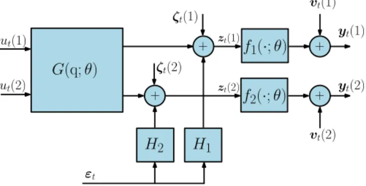
Block-oriented models (see [83, 167]) are models consisting of two main block types: static nonlinearity blocks and Linear Time-Invariant (LTI) dynamical blocks. The LTI blocks can be represented by parametric models such as rational transfer operators, linear state-space models, basis function expansions or by nonparametric models in either time or frequency domain. Similarly, the static nonlinearity can be represented by a nonparametric kernel model, or by some linear-in-parameters basis function model. A block-oriented model structure is developed by connecting several of these two building blocks together in series or in parallel, or both. Feedback connections are also possible. Although not as general as the Volterra representation or the NARMAX models, the block-oriented structures may be used to model many real-life nonlinear systems (see [83]). The simplest block-oriented structures are series connections involving only one block of each type, see Figure 1.2. A Wiener model is constructed by a single LTI block followed by a static nonlinearity block at the output; a Hammerstein model is constructed by a static nonlinearity block at the input followed by an LTI block. The model complexity can be increased by connecting these simple models in series or in parallel as shown in [83].

ut

vt

yt

+ LTI _NonlinearityStatic

(a) Wiener model: an LTI model followed by a static nonlinearity at the output

ut vt yt + LTI Static Nonlinearity

(b) Hammerstein model: a static nonlinear-ity at the input followed by an LTI model. Figure 1.2: A Wiener and a Hammerstein model.

One main advantage of block-oriented structures is the possibility of separat-ing the estimation of the linear and nonlinear parts of the model. Under some assumptions on the input signal and the noise, it is possible to construct best linear approximations (BLA) of the model, see [58, 154, 203, 204], which can be shown to be related to the LTI blocks, see [202, 205]. The main tool there is Bussgang’s theorem (see [23, Section III]); it states that the cross-correlation functions of a Gaussian signal before and after passing through a static nonlinear function are equal up to a constant. However, the constant may well be equal to zero (see Example 4.3 on page 75).

The choice among these different representations is usually guided by prior knowledge about the underlying system, the intended use of the model, and the available computational resources, among others. The selection of a model structure is fundamental to the system identification procedure and is recognized to be the most difficult step. Several specialized methods of structure selection for nonlinear models have been developed in both time and frequency domain, see for example [16] and [202].

The parameter estimation step for the model in (1.3) remains relatively simple. The ML problem can be easily formulated assuming a known distribution for vt

(31)

model include delayed measurement noise; the NARMAX model is defined by the relations

y_t= ψ(y_t₋₁, . . . , y_t_−n

y, ut−1, . . . , ut−nu, vt−1, . . . , vt−nv; θ) + vt, t∈ Z, for some ny, nu, nv∈ N. The values vt−1, . . . , vt−nv can be evaluated using the model, the initial conditions and the previous inputs and outputs (it is an invertible model). This allows us to compute the likelihood function in closed-form. Similarly, it is still possible to formulate a PEM problem in closed-form. A PEM estimator can be defined, for example, as the global minimizer

ˆ θ∶= arg min θ∈Θ N ∑ t=1 ∥yt− ψ(ϕ(t; θ); θ)∥ 2_.

Depending on the parameterization of the predictor function and the regression vector, the solution is usually not available in closed-form. The resulting optimization problem is in general non-convex. Nonlinear optimization algorithms like the damped Gauss-Newton algorithm or the Levenberg-Marquardt algorithm (see [68, 171, 173]) are therefore required. These algorithms are numerical iterative methods that can only find a local minimum. They require a good initial value to guarantee that the solution is in the vicinity of a global minimizer. In the case of block-oriented models, linear approximations can be used in some cases to initialize the optimization algorithms. There have been some research efforts in this direction, see for example [159, 176, 205, 208, 210, 211]. However, it should be noted that the problem of finding a linear approximation, depending on the chosen model structure for the LTI blocks, might still be a difficult non-convex problem.

To avoid possible local minima for complicated parameterizations, it is also possible to use random global search strategies such as simulated annealing and genetic algorithms (see [171, Chapter 5] or [190, Chapter 5]). However, due to their random nature, the exploration of the entire optimization domain could be computationally expensive and time-consuming. On the other hand, several approaches constrain the possible parameterization of the model in such a way that the resulting optimization problem has a closed-form solution (e.g., considering only linear-in-parameters models (see [209, Section 8] or [16, Chapter 3]).

A limitation

The model in (1.3) ignores any possible unobservable disturbance (different from

vt) that passes through the nonlinear dynamics. This is an idealization of the real

situation where there might exist a disturbance entering the system before some nonlinear subsystem. It has been shown in [99] that if the process disturbance is ignored, the resulting estimators will not be consistent. Therefore, it is important to develop identification methods that take into account the presence of such disturbances.

(32)

1.2.2 Case 2: Non-invertible Models

Suppose that the output does not only depend on the input and the variables vt,

but also on some (latent) unobserved process wtthrough a non-invertible (in wt)

nonlinear function. In this case, the output is given by

y_t= g(wt, ut; θ) + vt, t= 1, 2, 3, . . . (1.4)

in which g(⋅, ⋅; θ) ∶ R × R → R is a non-invertible (with respect to wt) nonlinear

function parameterized by θ.

Define the vector Wt ∶= [w1 . . . wt]⊺, let W ∶= WN, and assume that

W ∼ p(W ; θ) which has a known functional form. Let us first consider the ML

problem. Notice that in general the outputs{yt} are dependent over time; they are

independent over time only if the latent process w is independent over time. We also observe that because W is not observed, the PDF of Y has to be calculated by marginalizing the joint PDF p(Y , W ; θ) with respect to W ; that is

p(Y ; θ) = ∫

Rdw N

p(Y , W; θ) dW. (1.5)

Unfortunately, even though the integrand in (1.5) has a known form, the integral has no closed-form expression in general. The symbol dwdenotes the dimension of

the latent process w, which is assumed to be a scalar process in the current example (i.e., dw= 1). For commonly encountered models and applications, the value of dwN

isO(103_{) or O(10}4_{) and the evaluation of the integral in (1.5) is very challenging}

due to the nature of the integrand. To be able to find an approximate solution to the ML problem, one has to come up with computational methods that can approximate the maximizer of the intractable function p(Y ; ⋅) over a given set Θ.

During the last decade there has been several contributions in this direction; see for example [145, 172, 197, 244, 245] for ML estimation based on sequential Monte Carlo (SMC) methods. The survey [198] summarizes the available state-of-the-art algorithms and distinguishes between two main approaches: (i) the marginalization approach, and (ii) the data augmentation approach.

In the marginalization approach, SMC filters and smoothers (also known as particle filters) are used to “marginalize out” the latent process to approximate the logarithm of the likelihood function (the log-likelihood) and its gradient at a given value of θ. The resulting approximations are then used within an iterative numerical optimization algorithm to find an approximate solution to the ML problem. In the data augmentation approach, the SMC filters and smoothers are used in conjunction with the Expectation-Maximization (EM) algorithm (see [45]) to approximate the MLE as suggested in [239]. The resulting Monte Carlo EM (MCEM) algorithm converges only if the number of the Monte Carlo samples (particles) grows with the algorithm iterations, see for example [27, 71]. Furthermore, a new set of particles has to be generated at each iteration of the algorithm. In order to make a more efficient use of the particles, [44] suggested the use of a stochastic approximation version of the EM algorithm (SAEM) which replaces the expectation step of the

(33)

EM algorithm by one iteration of a stochastic approximation procedure. In [145], a particle Gibbs sampler (conditional particle filter with ancestor sampling, see [143]) is used within the SAEM algorithm to generate the required particles.

We note that the available convergence proofs of the MCEM and the SAEM algorithms (see [44, 71]) are, so far, given for cases where p(Y , W ; θ) belongs to the exponential family (see [195, Section 2.2] for a definition of the exponential family). This constrains the model parameterization and the distributions of w and v.

Estimation methods based on SMC approximations can be computationally expensive. For example, the convergence of the MCEM and the SAEM algorithms can be very slow when the variance of the latent process is small. Furthermore, cases with small or no measurement noise are quite challenging for SMC methods (see [224]). Moreover, due to the sample impoverishment and path degeneracy problems— a pair of fundamental difficulties of SMC methods (see [51, 52] and Chapter 3)—the SMC methods are so far, to the best of the author’s knowledge, applicable to models with relatively small dy and dw. In Chapter 3 we will give a brief overview of the

main ideas of these methods and highlight their properties.

The computations of a PEM estimator using the minimum MSE predictor, for cases with non-invertible model, are not easier than the computations of the MLE. The minimum MSE one-step-ahead predictor depends on the history of the observed outputs and is given by the conditional mean (see Chapter 2, page 35),

ˆ

y_t_∣t−1(θ) ∶= E[y_t∣Yt−1; θ] = ∫ Rdy

ytp(yt∣Yt−1; θ) dyt, t= 1, 2, 3, . . . (1.6)

where the PDF p(yt∣Yt−1; θ) is known as the predictive PDF and Y0 is defined

as the empty set; hence ˆy1∣0(θ) is constant and is equal to the expected value of y1. Unlike the MLE, the integrals appearing in the PEM objective function are of

the same dimension as that of the output signal. This means that the domain of the integrand is independent of N. For single-input single-output models (like the model in (1.4)), these are one-dimensional integrals; however, the integrand has an unknown form. Unfortunately, to be able to calculate the predictive PDF, we need to evaluate multidimensional integrals. Observe that by Bayes’ theorem (see [112, page 39]), p(yt∣Yt−1; θ) = p(Yt; θ) ∫Rdyp(Yt; θ) dyt = ∫Rdw tp(Yt, Wt; θ) dWt ∫Rdy∫Rdw tp(Yt, Wt; θ) dWtdyt . (1.7)

It appears that the predictive PDF of the output depends on p(Yt; θ) which does not

have a closed-form expression. To be able to formulate and solve a PEM problem, one has to come up with either consistent instances of the PEMs without relying on the minimum MSE predictor, or computational methods that can approximate the conditional mean (1.6). In the latter case, it seems that the PEM does not have any computational advantage over the efficient ML method. Both the MLE and the conditional mean of the outputs require the solution of similar marginalization integrals. For this reason, most of the recent research efforts found in the system identification literature, so far, target the maximum likelihood estimator.

(34)

One of the main contributions of this thesis is the introduction of one-step-ahead predictors constructed using the postulated statistical model without any reference to the data or the likelihood function (see Chapter 4). These predictors are relatively easy to compute and can be used, in many cases, to construct consistent instances of the PEMs. The predictors do not necessarily coincide with the minimum MSE pre-dictor, which means that certain asymptotic properties (such as statistical efficiency) cannot be guaranteed. However, the introduced predictors are algorithmically and conceptually simpler than predictors based on either SMC smoothing algorithms or Markov Chain Monte Carlo (MCMC) algorithms.

The main challenge

The two cases discussed above clarify the source of difficulty of the estimation problems considered in this thesis. The difference between the tractable model in (1.1) and the intractable model in (1.4) is the non-invertible nonlinear transformation of unobserved random variables in the latter. This makes the likelihood function and the minimum MSE one-step-ahead predictor of the output analytically intractable. Consequently, the objective functions of the optimization problems of both the MLE and the PEM estimator are not available in closed-form.

1.3 Thesis Outline and Contributions

The thesis concerns the estimation problem of stochastic parametric nonlinear dynamical models; a main objective is the construction and analysis of tractable estimators in different scenarios, when the models have intractable likelihood func-tions. The presented methods and examples are based on several published papers. Below we give an outline of the thesis and a description of the main contributions.

Chapter 2: Background and Problem Formulation

Chapter 2 provides the necessary background. Here, several important remarks and observations are made. After introducing a stochastic framework, a classical result on the structure of general second-order stochastic processes, due to Harold Cram´er in [39], is introduced. It generalizes Wold’s decomposition (see [246]) of stationary processes by giving a description of the second-order properties of a non-stationary process in terms of a causal linear time-varying filtering of the innovation process. This interesting result is used in Chapter 4 as the basis for optimal linear prediction of non-stationary processes with nonlinear underlying models. The chapter also reviews the ML method and the PEM. The kinship between the two approaches is highlighted using linear dynamical models. Finally, the main problem of the thesis is formulated.

(35)

1.3. Thesis Outline and Contributions 13

Chapter 3: Overview of Sequential Monte Carlo Methods

In this chapter, we give a short overview of several sampling-based approaches for ML estimation of general stochastic parametric nonlinear state-space models. They are based on sequential Monte Carlo and Markov chain Monte Carlo filtering and smoothing algorithms. Our objective here is to present the state-of-the-art methods and highlight some of their advantages and fundamental limitations. Finally, we clarify the differences to our approach.

Chapter 4: Linear Prediction Error Methods

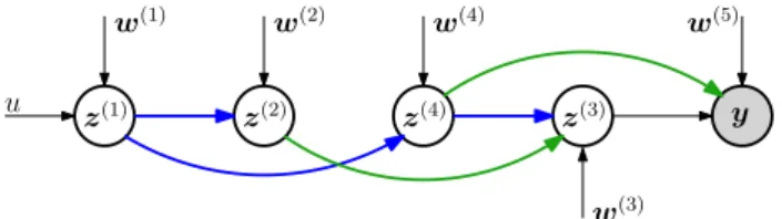
In this chapter, we introduce PEMs based on relatively simple predictors defined using the first and second moments of the hypothesized model. They are linear in the observed outputs, but are allowed to depend nonlinearly on the (assumed known) inputs. It is shown that for several relevant models with intractable likelihood functions (such as stochastic block-oriented models with polynomial nonlinearities), the proposed PEM estimators are defined by closed-form (exact) expressions. We also observe that this will be the case for a class of nonlinear dynamical networks. The convergence of the resulting estimators is established under suitable regularity conditions, and consistency is proven under certain identifiability condition. The chapter also clarifies the relation between the proposed estimators and those based on second-order equivalent models ([58, 154]). The performance of the methods is illustrated by numerical simulations using several challenging models, in addition to a recent real-data benchmark problem.

The content of this chapter is based on the following peer-reviewed published articles:

● M. Abdalmoaty and H. Hjalmarsson. Linear prediction error methods for stochastic nonlinear models. Automatica, 105:49-63, 2019.

● M. Abdalmoaty and H. Hjalmarsson. Application of a linear PEM estimator to a stochastic Wiener-Hammerstein benchmark problem. In IFAC-PapersOnLine, Volume 51, Issue 15, pp. 784–789, 2018.

● M. Abdalmoaty, C. R. Rojas, and H. Hjalmarsson. Identification of a class of nonlinear dynamical networks. In IFAC-PapersOnLine, Volume 51, Issue 15, pp. 868–873, 2018.

● M. Abdalmoaty and H. Hjalmarsson. Consistent estimators of stochastic MIMO Wiener models based on suboptimal predictors. In the 57th IEEE

Conference on Decision and Control (CDC), pp. 3842-3847, 2018.

Some parts and examples can also be found in Chapter 4 in

● M. Abdalmoaty. Learning Stochastic Nonlinear Dynamical Systems Using Non-stationary Predictors. Licentiate dissertation, KTH Royal Institute of Technology, Automatic Control Department, 2017.

(36)

Chapter 5: Simulated Linear Prediction Error Methods

In this chapter, we present simple Monte Carlo approximation methods that may be used whenever the linear predictors defined in Chapter 4 are analytically intractable. They are based on plain Monte Carlo simulations of the model and come with several favored properties. For example, the Monte Carlo error is independent of the dimension of the model. Moreover, the continuity of the approximated criterion functions may be ensured by using common random numbers. This is particularly important for the numerical optimization procedure, and allows us to establish the convergence of the estimators. We use numerical simulation examples to illustrates the properties of the method and compare to the current state-of-the-art algorithms. Finally, a comparison and a connection are made to a PEM based on the Ensemble Kalman filter (a Monte Carlo filter used to define a (nonlinear) suboptimal predictor).

Parts of this chapter are based on the published peer-reviewed article

● M. Abdalmoaty and H. Hjalmarsson. Simulated pseudo maximum likelihood identification of nonlinear models. In IFAC-PapersOnLine, Volume 50, Issue 1, pp. 14058–14063, 2017.

and Sections 4.6 and 4.7 in

● M. Abdalmoaty. Learning Stochastic Nonlinear Dynamical Systems Using Non-stationary Predictors. Licentiate dissertation, KTH Royal Institute of Technology, Automatic Control Department, 2017.

Chapter 6: Identification Using Optimal Estimating Functions

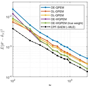
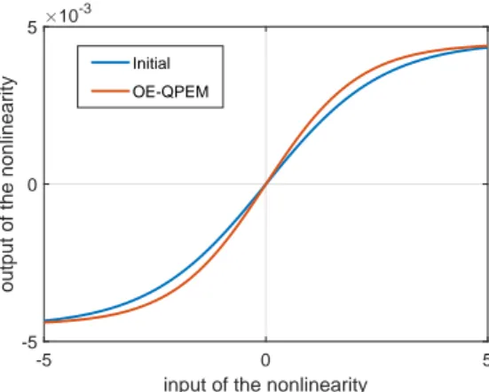
In this chapter, we examine the asymptotic properties of the linear PEMs introduced in Chapter 4 when quadratic criteria are used. We show that a PEM based on a Gaussian assumption, where the mean vector and covariance matrix are jointly parameterized, is not necessarily more accurate than an optimally weighted output-error PEM (where the parameterized covariance matrix is not used). Thus, the Gaussian assumption comes with no support or motivation. We then introduce the estimating functions approach, which was almost entirely developed in the statistics literature (see [56, 88, 90, 105]). We present a method that may be used to systematically construct asymptotically uniformly optimal estimators among a class of estimators including all linear PEM estimators with quadratic criteria. The convergence and consistency of the estimators are established under suitable conditions similar to those used in Chapter 4. We clarify the connection between the estimating function approach and the prediction error correlation approach. The chapter is concluded with several analytical and numerical simulation examples.

The content of this chapter is based on the following article:

● M. Abdalmoaty and H. Hjalmarsson. Identification of stochastic nonlinear models using optimal estimating functions. In Automatica. Under review for

(37)

1.3. Thesis Outline and Contributions 15

Chapter 7: Closed-Loop Identification

The methods developed in Chapters 4-6 are based on the assumption that the input is known and independent of all disturbances and measurement noises; hence, the system is necessarily operating in open-loop. In this chapter, we consider cases where the data is collected under closed-loop operation. We study two scenarios given by the assumptions on the disturbances, measurement noise and the knowledge of the feedback mechanism, where the attention is given to the consistency of the estimators. The methods can be regarded as generalizations of classical closed-loop identification methods of linear time-invariant systems. We provide an asymptotic analysis of the proposed method and demonstrate their consistency on a simple simulation example.

The content of this chapter is based on an article under preparation:

● M. Abdalmoaty and H. Hjalmarsson. Closed-loop identification of stochastic nonlinear models. To be submitted to Automatica as a regular paper.

Chapter 8: Conclusions and Future Research Directions

In this last chapter, we summarize the conclusions of the thesis and give some pointers for future research.

Appendices

The thesis contains four appendices where relevant definitions and results are summarized. The first three are edited republication of those in [3]. Appendix A introduces the idea of Monte Carlo estimation. Random sampling, common random numbers, rejection and importance sampling, and Markov chain methods are described. In Appendix B, Hilbert spaces of random variables are defined and the linear minimum mean-square error predictors are derived based on the projection theorem. Appendix C gathers some relevant properties of Gaussian random vectors and multivariate Gaussian distributions. Lastly, Appendix D contains a classical uniform convergence result, which is used in the proof of Theorem 5.1.

(38)

(39)

Chapter 2

Background and Problem Formulation

This chapter introduces the necessary background, makes several remarks, and formulates the main problem. We start by introducing a stochastic framework for the signals and then describe the models that we are concerned with. We then discuss several statistical estimation methods and their properties. Finally, we formulate the main problem of the thesis.

2.1 Mathematical Models

The mathematical models considered in this thesis belong to the set of stochastic models: all the signals are modeled as stochastic processes. A stochastic process

y= {y_t∶ t ∈ T} is a family of random variables, indexed by a given index set T, and

defined over a probability space(Ω, F, Pθ). In this thesis, the probability measure

is parameterized by a finite-dimensional real vector θ∈ Θ ⊂ Rdθ, d

θ∈ N. The index t

always corresponds to time, and the index set T is taken as the set of integers Z giving rise to discrete-time stochastic processes (see [47]). Let t1, t2, . . . , tN be an

arbitrary finite sequence of integers. Then the joint probability distribution of the random variables yt1, . . . , ytN in y is known as a finite-dimensional distribution of the process y. The probability measure Pθ can be characterized by specifying all

the finite-dimensional probability distributions.

The mathematical models are deterministic functions that define the probability measure Pθon the space of observed signals. Because all practical systems are causal

systems, for which the current output does not depend on the future inputs or future disturbances, we limit ourselves to causal models. For every t, we always assume the existence of a joint probability density function p(Yt; θ) of the vector

Yt∶= [y⊺1, . . . , y⊺t]⊺. We start by defining special classes of signals.