Nr 70 . 1982 » ,
ISSN 0347-5049 '_ 'The"Regressron-to-mean"Effect
Statens väg- och trafikinstitut (VTI) '. 581 01 Linköping
National Road & Traffic Research Institute ' S-581 0,1 Linköping; ' Sweden
omeempiricalexamplesconcerning
slgaccrdentsatroadjunctions
" *
_ byUlfBrudeandJorgenLarsson
& ,. f ..
j;._jgjff);'(MeasurementsofDegreeotSeparation
(_
BetweenVe? 'i alesandPedestrians
.
i,;m UrbanAreas
* "ff . Til'YGoranNllSSOnandHansThulm
._ ';';.'Å_V'_;"Repr1ntsof paperspresentedat themternatlonalOECDSemmaronShortterm lgfllif
land AreawrdeEvaluatlonofSafetyMeasuresAmsterdam theNetherlandsApnlh; _A
"19211982 _. , . . . ___ _ _ _ ,. * ;_4 ,"f' v. . ..._; . ' , ., _ . _ " ,, __ 7.11 ..: _ ."_. _ ' ' - . . ,_ . _ .-* .:-' __»,-.. ,» _ , -...' ;. '. x.J.;»;-. 2', : .» .V'.. _ . .. : . » -». .v. ' ,.3 .- _' ( x; ' . ., , - . , _ ', : . ,. , . », .=' . _ . . - _ . . A. .. , . . . _ _. _ ,. ___..._!.l_ . J . : " ' . .» "I": ., . ' . ' _ -_ ."**._"., oW-"z' , j . ,, '. .= w. * p , _ _ __ . _ _ _ _ , ; _ , ..; _ « » . x * f ' * ' . '_, ' i ' * . ,
SAR TRCCEIK
Nr 70 ' 1982 Statens väg- och trafikinstitut (VTI) ' 581 01 Linköping
ISSN 0347-6049 National Road & Traffic Research Institute ' S-581 01 Linköping ' Sweden
The "Regression to-mean" Effect
Some empirical examples concerning
accidents at road iunctions
by Ulf Briide and Iörgen Larsson
Measurements of Degree of Separation
Between Vehicles and Pedestrians
in Urban Areas
by Göran Nilsson and Hans Thulin
Reprints of papers presented at the international OECD Seminar on "Short-term and Area-wide Evaluation of Safety Measures", Amsterdam, the Netherlands, April
7 o 19 21 1982.
National Swedish Road and Traffic Research Institute
5 581 01 Linköping
Sweden
THE "REGRESSION-TO-MEAN" EFFECT
Some empirical examples concerning accidents at road junctions by Ulf Brijde and Jörgen Larsson
ABSTRACT
A randomly large number of accidents during a "before-period" is normal
ly followed by a reduced number of accidents during a corresponding "after period" even if no countermeasures have been implemented. This
statistical phenomenon is termed the "regressiomto-mean" effect (or
shorter the regression effect).
Road junctions constitute points in the road network with particularly high accident rates although the average number of accidents per junction is low. The latter means that the regression effect can be expected to appear even in very modest accident numbers.
The examples described in this report are based on accidents at unaltered rural junctions in the national major road network. The years 1972-1975 have been regarded as the before period and 1976 1978 as the after period.
The examples show that the regression effect (accident reduction) in
accidents reported to the police often can be about 30-40 %. For
accidents involving personal injury the regression effect is often about
50 60 %. In the case of junctions with a significantly large number of accidents (in relation to the amount of traffic) during the before period the regression effect is usually even greater.
INTRODUCTION
A randomly large number of accidents during a before-period is normally followed by a reduced number of accidents during a corresponding after-period even if no countermeasures have been implemented (and a randomly small number of accidents is normally followed by an increased number of accidents). This statistical phenomenon is termed the "regres
sion-to-mean effect* (or shorter the regression effect). An earlier article (l) describes examples which show that: 0 the regression effect can be very large
o the regression effect can have an entirely decisive influence on the
results of before-and after studies.
The objective of this report is to describe some examples of the regression effect in more detail.
The project was financed by the National Road Administration.
SOME EXAMPLES OF "REGRESSION-TO-MEAN" EFFECT OF ACCIDENTS AT UNALTERED ROAD JUNCTIONS
Comments relating to Tables 1-5:
The tables are based on 2637 rural road junctions* in the national major road network which were unaltered from 1972 to 1978**.
The ll year period 1972-1975 has been regarded as the before period and the 3-year period 1976 1978 as the after-period.
Tables 1, 2 and 5 relate to police-reported accidents including both
personal-injury and property damage accidents.
Tables 3 and 4 relate only to personal-injury accidents.
The annual amount of traffic was on average 13.6 % greater during
1976 1978 than during 1972-1975. However, the annual number of
police-reported accidents was on average about 15.5 % greater during
1976-1978 than during 1972-1975 (Table 1***). The annual number of
personal-injury accidents was on average about 16 % greater during
1976 1978 than during 1972 1975 (Table 3****).
In these calculations the number of accidents for 1972-1975 has been
multiplied by å ' 1.136 in order to obtain a comparison between the
number of accidents for 1972 1975 and 1976-1978.
**
A speed limit of ; 70 km/h in force on every national connecting road. Straight primary road, stop sign. No pedestrian or cycle path
and no traffic signals.
According to information from the 1977-1978 inventory of junc-tions, updated to 3lst of December 1978.
*** 1896/ M 21.155
****704/
q
The average number of Police-reported accidents per junction and xear for 1972 1975 was 0.21 (Table 1*). This means that junctions with 1 police reported accident during this 4-year period had a greater accident number than average.
The average number of personal-injury accidents per junction and
year during 1972-1975 was 0.08 (Table 3**). This means that
junctions with 1 personal-injury accident during this 4 year period had an accident number about 3 times greater than average.
According to Table 1 there were, for example, 4 police-reported
accidents per junction at 53 junctions (a total of 212 accidents)
during 1972 1975. A total of 103 police-reported accidents occured
at the same junctions during 1976-1978. The accident reduction
between the before period and after-period (the estimated
regres-sion effect) was therefore 212 ° 3 ' 1.136
q
(1-103/ )-100%=#3%
For police reported accidents (Table 1) the estimated regression
effect is on average just over 35% provided that at least 2 accidents occurred during the before-period. Where there occurred l police reported accident during 1972-1975 the estimated regres
sion effect is on average about 10 % (Table 1).
For personal injury accidents (Table 3) the estimated regression effect is on average just over 55 % provided that there occurred at
least 2 personal-injury accidents during the before-period. It is
notable that the estimated regression effect is on average about
50 % even in the case where there occurred only l personal-injury
accident during 1972 1975 (Table 3).
2189 2637 11 809 637' = 0.21 .O o 00 N _D
The fact that the regression effect becomes greater for personal-injury accidents than for all police-reported accidents is theoreti-cally to be expected, since the personal-injury accidents are on a
lower numeric level and thus have a relatively greater standard deviation in relation to the mean (assuming that the accidents
follow the Poisson distribution).
In Tables 1 and 3 it should also be _n_c_>t_e_c_l that the junctions with O accidents during the before-period account for a very large propor-tion (about one third and one half respectively) of the total number
of accidents during the after-period. In this case there is a
regression effect from the opposite direction, i.e. an accident
increase.
If a study is made of only those junctions which, according to the
Institute's models*(2), had a significantly higher number of police reported accidents than expected (level of significance 2.5 %) during
the before-period the estimated regression effect increases to an average of about 65 % (Table 5). For personal injury accidents the estimated regression effect in corresponding cases can be seen to increase to an average of about 75 %.
It must be remembered that the examples mentioned here apply to
the case where the before-period covers 4 years. If a shorter
before-period had been chosen, the estimated regression effects would have been even greater.
For junctions with significantly more police reported accidents than expected during 1972 1975 Table 5 allows a comparison to be made between the number of accidents actually reported to the police for l972-l975 and for 1976 1978 respectively, with the predicted (ex pected) number of accidents according to the Institute's models. It can be seen that even during the after-period (i.e. after the number of accidents has regressed towards its true means) the
The models relate to type (3 or 4-way junction),number of entering
vehicles (pair of axles) from primary and secondary roads and
recorded number of accidents is on average considerably larger than predicted. It would therefore not have been an incorrect decision, seen as an average, to attempt to modify these junctions on the
basis of the significantly high accident numbers recorded during
1972-1975. In this case, however, it would have been impossible to estimate correctly the possible accident reduction effects of
individual countermeasures.
If those junctions in a specific road network having ak accidents during a before period are selected, it may be expected, assuming that no countermeasures are taken, that during a corresponding after-period the number of accidents at these junctions will equal the total number of accidents at those junctions which had ; (k+l)
accidents during the before-period. This ingenious yet simple
method has been introduced by Hauer (3,4).
It can be seen that the recorded number of accidents for 1976-1978 agrees very well with the number which may be expected according to Hauer's method* (Tables 2 and #).
When calculating the expected number of accidents according to
Hauer's method correction has been made by multiplying with the
factor % - 1.136.
Ta bl e 1. Ju nc ti on s wh ic h, du ri ng 19 72 19 75 , ha d: a Pr ed . no . of ac ci de nt s 19 72 19 75 ac co rd in g to mo de l b Re co rd ed no . of ac ci de nt s 19 72 19 75 c Re co rd ed no . of ac ci de nt s
19
72
-1
97
5
ad
ju
st
ed
to
be
co mp ar ab le ag ai ns t th e re co r-de d no . of ac ci de nt s 19 76 19 78 d Pr ed ic te d no . of Re co rd ed no . ac ci de nt s 19 76 -19 78 ac cord in g to mo de l 2) e of ac ci de nt s 19 76 -1 97 8 Po li ce -r ep or te d ac ci de nt s. Ru ra l ju nc ti on s in th e ma jo r road ne tw or k wh ic h we re un al te re d du ri ng 19 72 -1 97 8. 8 Es ti ma te of th e re gr es si on ef fe ct _C CDI'O 27 ac ci de nt s (2 6 ju nc ti on s) 6 ac ci de nt s (1 7 ju nc ti on s) 5 ac ci de nt s (3 9 ju nc ti on s) 4 ac ci de nt s (5 3 ju nc ti on s) 3 ac ci de nt s (1 01 ju nc ti on s) 2 ac ci de nt s (2 44 ju nc ti on s) 1 ac ci de nt (6 57 ju nc ti on s) O ac ci de nt s (1 50 0 ju nc ti on s) 76 .1 44 .8 93 .4 97.5 159. 1 30 1. 0 56 7. 4 76 1. 2 23 2 10 2 19 5 21 2 30 3 48 8 65 7 19 7. 7 86 .9 16 6. 1 18 0. 6 25 8. 2 41 5. 8 55 9. 8 64 .8 38 .2 79 .6 83 .1 13 5. 6 25 6. 5 48 3. 4 64 8. 5 14 2 52 10 5 10 3 18 1 25 3 50 9 55 1 0. 72 0. 60 0. 63 0. 57 0. 70 0. 61 0. 91 28 % 40 % 37 % 43 % 30 % 39 % 9 % 1. 36 1. 32 1. 24 1. 33 0. 99 1.05 0.85 To ta l (2 63 7 ju nc ti on s)1)
Mu
lt
ip
li
ed
by
2) Pr ed ic te d nu mb er of ac ci de nt s du ri ng 19 72 19 75 ac co rd in g to th e mo de l mu lt ip li ed by 3 4 21 00 .5 21 89 18 65 .1 17 89 .6 18 96 ' 1. 13 6 (a n av er ag e of 13 .6 % mo re tr af fi c pe r ye ar du ri ng 19 76 -1 97 8 th an du ri ng 19 72 19 75 ) 3 4 1. 13 6 1. 02Ta bl e 2. Poli ce re po rt ed ac ci de nt s. Ru ra l ju nc ti on s in th e majo r ro ad ne tw or k wh ic h we re un al te re _d du ri ng 19 72 19 78 . a b c Ju nc ti on s wh ic h, du ri ng Re co rd ed no . Re co rd ed no . of ac ci de nt s Re co rd ed no . Es ti ma te of No . of ac ci de nt s 19 72 19 75 , ha d: of ac ci de nt s 19 72 19 75 ad ju st ed to be of ac ci de nt s th e re gr es si on 19 76 19 78 pr ed ic te d 1972 -1 97 5 co mp ar ab le ag ai ns t th e re co r 19 76 19 78 ef fe ct by "H au er 's me th od " de d no . of ac ci de nt s19 76 19 78 e f "O U|..O l\ AX ac ci de nt s (2 6 ju nc ti ons) 23 2 19 7.7 14 2 0. 72 28 % 10 8. 2 NO /\\ ac ci de nt s (4 3 ju nc ti on s) 33 4 28 4. 6 19 4 0. 68 32 96 19 7. 7 lm /\\ ac ci de nt s (8 2 ju nc ti on s) 52 9 45 0 .7 29 9 0 .6 6 34 96 28 4 .6 ;t-/\\ ac ci de nt s (1 35 ju nc ti on s) 74 1 63 1. 3 40 2 0. 64 36 % 45 0. 7 m /\\ ac ci de nt s (2 36 ju nc ti on s) 10 44 88 9. 5 58 3 0. 66 3 96 63 1. 3 >, 2 ac ci de nt s (480 ju nc ti on s) 15 32 1305 .3 83 6 0. 64 36 96 88 9. 5 ac ci de nt (1 13 7 ju nc ti on s) 21 89 18 65 .0 13 45 0. 72 28 % 13 05 .3 v ( /\\ >/ 0 ac ci de nt s (2 63 7 ju nc ti on s) 21 89 18 65 .0 18 96 18 65 .0 '_1) Mu li pl ie d by å ° 1. 13 6 (a n av er ag e of 13 .6% mo re tr af fi c pe r ye ar du ri ng 19 76 19 78 th an du ri ng 19 72 -197 5)
Ta bl e 3. Pe rs on al mi nj ur y ac ci de nt s. Ru ra l ju nc ti on s in th e ma jo r road ne tw or k wh ic h we re un al tere d du ri ng 19 72 -1 97 8. a b c Ju nc ti on s wh ic h, du ring Re co rd ed no . Re co rd ed no. of ac ci de nt s Re co rd ed no . Es ti ma te of l9 72 l9 75 ,h ad : of ac ci de nt s 19 72 -1 97 5 ad ju st ed to be ofac ci de nt s th e re gr es sion 19 72 19 75 co mp ar ab le ag ai ns t th e re co r 19 76 19 78 ef fe ct de d no . of ac ci de nt s19 76 19 78 e O OLD >, 4 ac ci de nt s(l 4 ju nc ti on s) 58 49 .4 21 0. 43 57 % 3 ac ci de nt s (2 4 ju nc ti ons) 72 61 .3 32 0. 52 4 8 % 2ac ci de nt s (1 19 ju nc ti on s) 23 8 20 2. 8 84 0. 41 59 °/ o l acci de nt (4 41 ju nc ti on s) 44 1 37 5. 7 18 4 0. 49 51 % 0 ac ci de nt s (2 03 9 junc ti on s) 0 0 38 3 To ta l (2 63 7 ju nc ti ons) 80 9 689 .3 70 4 l.02 3 l) Mu lt ip li ed by 4 -1.13 6 (a n av er ag e of 13 .6 % more tr af fi c pe r ye ar du ri ng 19 76-1 97 8 th an du ri ng 19 72 -1 97 5)
Ta bl e 4. Pe rs on a1 in ju ry ac ci de nt s. Ru ra l ju nc ti on s in th e ma jo r ro ad ne tw or k wh ic h we re un al te re d du ri ng 19 72 19 78 . a b c e f Ju nc ti on s wh ic h, du ri ng Re co rd ed no . Re co rd ed no . of ac ci de nt s Re co rd ed no . Es ti ma te of No . of ac ci de nt s 19 72 -1 97 5, ha d: of ac ci de nt s 19 72 19 75 ad ju st ed to be of ac ci de nt s th e re gr es si on 19 76 19 78 pr e 19 72 -1 97 5 co mp ar ab le ag ai ns t th e re co r 19 76 19 78 ef fe ct di ct ed by d e d no . of ac ci de nt s 1 9 7 6 -1 9 7 8 Ha ue r' s m e t h o d " 'D ULO >, 4 ac ci de nt s (1 4 ju nc ti on s) 58 49 .4 21 0. 43 57 % >, 3 ac ci de nt s (3 8 ju nc ti on s) 13 0 11 0. 8 53 0. 48 52 % 49 .4 >, 2 ac ci de nt s (1 57 ju nc ti on s) 36 8 31 3. 5 13 7 0. 44 56 % 11 0. 8 >/ 1 ac ci de nt (5 98 ju nc ti on s) 80 9 68 9. 3 32 1 0. 47 53 % 31 3. 5 >, 0 ac ci de nt s (2 63 7 ju nc ti on s) 80 9 68 9. 3 70 4 -68 9. 3 1) Mu lt ip li ed by å ' 1. 13 6 (a n av er ag e of 13 .6 96 mo re tr af fi c pe r ye ar du ri ng 19 76 19 78 th an du ri ng 19 72 -1 97 5)
Ta bl e 5. Po li ce re po rt ed ac ci de nt s. Ru ra l ju nc ti on s in th e ma jo r ro ad ne tw or k wh ic h we re un al te re d duri ng 19 72 19 78 an d wh ic h, ac co rd in g to th e In st it ut e' s mode ls , ha d a si gn if ic an tl y hi gh er nu mb er of. po li ce-r ep or te d ac ci de nt s th an ex pe ct ed du ri ng 19 72 19 7 5. a b c d e f g Ju nc ti on s Pr ed ic te d no . Re co rd ed no . Re co rd ed no . of ac ci de nt s Pr ed ic te d no . of Re co rd ed no . _e_ Es ti ma te of wh ic h, du ri ng of ac ci de nt s of acci de nt s 19 72 19 75 ad ju st ed to be ac ci de nt s 19 76 -of ac ci de nt s c th e re gr es si on 19 72 19 75 , 19 72 19 75 19 72 19 75 co mp ar ab le ag ai ns t th e re co r-19 78 ac co rd in g 19 76 -1 978 ef fe ct ha d: ac co rd in g to de d no . ofac ci de nt s 19 76 19 78 to mo de lZ ) mo de l £: CDI O 37 ac ci de nt s 52 .2 18 9 16 1. 0 44 .5 10 4 0. 65 35 % 2. 34 (2 1 ju ncti on s) 6 ac ci dent s 13 .4 48 40 .9 11 .4 19 0. 46 54 96 1. 67 (8 ju nc ti on s 5 acci de nt s 25 .6 85 72 .4 21 .8 31 0.43 57 % 1. 42 (1 7 ju nc ti on s) # ac ci de nt s 28 .7 10 4 88 .6 24 .5 25 0. 28 72 % 1. 02 (2 6 ju nc ti on s) 3 ac ci de nt s 23 .9 10 5 89 .5 20 .4 25 0. 28 72 96 1.23 (3 5 ju nc ti on s 2 ac ci de nt s 15 .7 80 68 .2 13 .4 23 0. 34 66 96 1. 72 (4 0 ju nc ti ons) la cc id en t 4. 6 31 26 .4 3. 9 5 0. 19 81 % 1. 28 (3 1 ju nc ti on s) 10 To ta l 16 4. 1 64 2 54 7. 0 13 9. 8 23 2 0. 42 58 % 1. 66 (1 78 junc ti on s) l) Mu lt ip li ed by å-1. 13 6 (a n av er ag e of 13 .6 96 mo re tr af fi c pe r ye ar duri ng 19 76 19 78 th an du ri ng 19 72 -1 97 5) 2) Pr ed ic te d nu mb er of ac ci de nt sdu ri ng 19 72 -1 97 5 ac co rd in g to th e mo de lmu lt ip li ed by å -1. 13 6
11
HOW CAN THE "REGRESSION TO-MEAN" EFFECT BE ADJUSTED IN NON-EXPERIMENTAL BEFORE-AND-AFTER STUDIES?
On the basis of the results described in Chapter 2 information is obtained on the average magnitude of the regression effect at road junctions in the
Swedish major road network for different accident numbers during a
before-period covering # years. Hauer's method provides in more general terms a possibility for estimating the average regression effect for groups of selected objects.
From the practical aspect it is especially desirable to be able to estimate
the regression effect for investigated objects (e.g. junctions) either
individually or in small groups.
For the 2637 unaltered junctions already studied subsequent processing
has shown that
o it may be appropriate to have the before-period to cover 5 years
. it may also be appropriate to omit a certain number of the worst
accident years (the year/years with the greatest number of acci dents) and instead to allocate these years the average number of accidents per year for the other years.
With this procedure it should be possible to make a rough but individual correction for the regression effect.
The following table shows that, for junctions which had significantly more police-reported accidents in 1972 1976 than expected (level of signifi-cance 2.5 %) according to the Institute's models and at the same time at least 5 police reported accidents during this period, it would be necessary
on average to omit the 2 worst years during the before-period in order to
obtain approximately the same number of accidents per junctions and year as for the after-period l977-l978*.
* Attention has been paid to the fact that the average annual amount
of traffic was about 12.6 % greater during 1977-1978 than during
12
For those junctions which, according to the Institute's models, had
significantly more police-reported accidents during 1972-1976 than ex
pected but fewer than 5 police reported accidents it would seem more
appropriate to omit only the worst accident year.
Junctions (unaltered during 1972-1978) with significantly more police reported
acci-dents than expected for 1972-1976:
a b c d
Junctions 1972- 1976, 1972- 1976 1972 1976 1977- 1978,
which, during no. of excl. the excl. the no. of
1972-1976, accidents per worst acci 2 worst accidents
had junction dent year, accident per junction
and year* no. of years, no. of and year
accidents accidents
per junction per junction
and year* and year*
310 accidents 3.15 2.51 1.94 1.88 (12 junctions) 9 accidents 2.03 1.58 1.35 1.10 (5 junctions) 8 accidents 1. 80 1. 44 1. 08 1. 00 (8 junctions) 7 accidents 1. 58 1.09 0.70 1.07 (7 junctions) 6 accidents 1.35 0.92 0.68 0.64 (11 junctions) 5 accidents 1.13 0.74 0.57 0.39 (19 junctions) 4 accidents 0 . 90 0 . 50 0 . 27 0 . 56 (26 junctions) 3 accidents 0.68 0.35 0.13 0.26 (29 junctions) 2 accidents 0.45 0.23 0.00 0.19 (37 junctions) 1 accident 0.23 0.00 0.00 0.03 (18 junctions)
* Multiplied by 1.126 since the average annual amount of traffic was 12.6 °/o greater
13
For those junctions which, according to the Institute's models, had more, but not significantly more, police reported accidents than expected it would be too drastic to omit the worst accident year. Instead, it would be better to take the "mean" of not omitting any accident year and omitting the worst accident year.
Junctions (unaltered during 1972 1978) with more, but not significantly more, police-reported accidents than expected for 1972-1976:
a b c d
Junctions 1972-1976, 1972-1976 a + b 1977-1978,
which, during no. of excl. the 2 no. of
1972-1976, accidents per worst acci- accidents
had junction dent year, per junction
and year* no. of and year
accidents per junction and year* 17 accidents 3.82 3.10 3.46 5.50 (1 junction) 8 accidents 1.80 1.48 1.64 1.50 (4 junctions) 7 accidents 1. 58 1.00 1.29 1.23 (11 junctions) 6accidents 1.35 0.89 1.12 1.13 (12 junctions) 5 accidents 1.13 0.73 0.93 0.75 (24 junctions) 4accidents 0.90 0.52 0.71 0.71 (42 junctions) 3 accidents 0.68 0.36 0.52 0.41 (81 junctions) 2 accidents 0.45 0.21 0.33 0.28 (205 junctions) l accident 0.23 0.00 0.12 0.12 (391 junctions)
* Multiplied by 1.126 since the average annual amount of traffic was 12.6 % greater during 1977 1978 than during 1972-1976.
14
For junctions with more (not necessarily significantly more) personal
injury accidents than expected* it would seem appropriate to take the
"mean" of omitting the worst accident year and omitting the two worst
accident years. For personal-injury accidents the pattern in a procedure of this nature will however not be as clear as that described for police-reported accidents on pages 12 and 13 .
A procedure following that described above is conceivable at least for
road junctions in the Swedish major road network. The advantages of this method are that it is both very simple and that the regression effect is
treated individually for each junction. The disadvantage is that the
method is rough and especially that it is not in any way supported by theory.
15 REFERENCES
(l)
(2)
(3)
(4)
Briide U (1981):
"Trafiksakerhetsstudier -kan man lita på resultat av
före-efter-studier?"
Väg- och vattenbyggaren december l98l/VTI Särtryck 1982
("Traffic safety how reliable are before-and-after studies?", an unpublished translation of the above-mentioned article, VTI)
Briide U och Larsson J (1981):
"Vägkorsningar på landsbygd inom huvudvägnätet, olycksanalys"
VTI Rapport 233
Briide U and Larsson J (1981):
"Rural junctions in the main road network, accident analysis" VTI Report 233
Hauer E (1980):
"Bias by selection: Overestimation of the effectiveness of safety countermeasures caused by the process of selection for treatment" Accident analysis & Prevention Vol 12
Hauer E (1980):
"Selection for treatment as a source of bias in
before-and-after-studies"
MEASUREMENTS OF DEGREE OF SEPARATION BETWEEN VEHICLES AND PEDESTRIANS IN URBAN AREAS.
by
Göran Nilsson and Hans Thulin
National Swedish Road and Traffic Research Institute 5-581 01 LINKÖPING
Sweden
ABSTRACT
Most measures in order to increase traffic safety for unprotected road users are measures which separate vehicles from pedestrians or bicyclists in time or space.
This paper presents some results from emperical studies at pedestrians
crossing concerning the proportion of pedestrians who can cross the street
without disturbing or being disturbed by vehicles. This proportion of
pedestrians is defined as the degree of separation between vehicles and pedestrians. Video technics were used for the measurements.
Both theoretical calculations and emperical measurements of the degree
of separation have been made for the central part of Linköping at 16
randomly chosen pedestrian crossings.
The observation period at each crossing was 90 minutes distributed on three 30-minutes periods during daytime for three weekdays. From this it
has been possible to estimate the traffic composition during different
hours of the day for the central part of the city.
By comparing the total degree of separation of pedestrians during different periods of the day and accidents for the corresponding periods, relationships between risk (number of collisions between vehicles and pedestrians per pedestrian and pedestrian crossing) and pedestrian flow for different degrees of separation have been calculated.
BACKGROUND
On behalf of the National Road Board the National Road and Traffic Research Institute (VTI) is developing different risk estimates concerning unprotected road users in urban areas.
As most of the measures to increse traffic safety for unprotected road users are based on separation/segregation between motor vehicles and pedestrians or bycyclist/mopedists, the research has been directed to deve10p methods to make quantitative measurements of the magnitude of separation in different locations in urban areas.
The results presented in this paper are preliminary but give some examples concerning the separation between pedestrians and motor
vehic-les and risk calculations for pedestrian crossing in the central part of a
city.
METHOD
The central part of Linkoping was defined and 16 pedestrian crossings
were chosen at random.
This procedure makes it possible to estimate the traffic composition on pedestrian crossings in the centre of the city. Video technics were used
for the measurements. The measurements were made during three
weekdays at three different times on every pedestrian crossing. The
observation period at each crossing was 90 minutes distributed on three randomly chosen 30-minutes periods during daytime.
Each pedestrian crossing has been evaluated concerning
. pedestrian flow (pedestrian/h) in different directions on the pedestrian crossing
. motor vehicle flow for different types of vehicles
In the next phase every pedestrian has been observed during the passage
of the pedestrian crossing. This has been divided into two parts
(separation areas). One deals with the first half of the passage and the
other with the second half. For both the first and the second part it was noted if a motor vehicle was going to drive across the pedestrian crossing
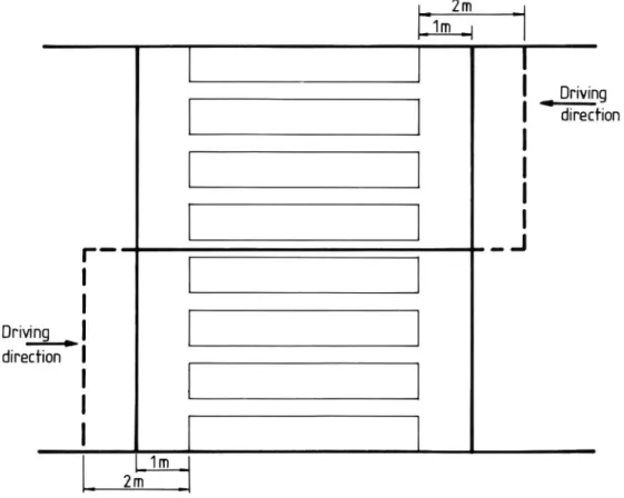
or not. The separation areas are marked by unbroken lines (fig. 1). Broken
lines mark the boundary for passing motor vehicles. The pedestrian is
considered as non-separated and non-disturbed by motor vehicles, if, at the same time both a pedestrian and a motor vehicle are in the separation area or the motor vehicle is within the broken line preceding the separation area. 2m _ 1m | | Driving | direction
I
I
I"
_ J
I
I
Driving | direction |I
I
1m 2m _Figure l. Pedestrian crossing and separation area.
The number of pedestrian observations without any disturbing motor
vehicle(s) in relation to the total number of pedestrian observations is defined as the degree of separation for pedestrians.
Traffic safety and traffic composition
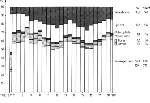
The observations of the hourly flow of passenger cars, lorries, buses, motorcycles, mopeds, cyclists and pedestrians resulted in estimates of the traffic composition between 0630 and 1830. These estimates are
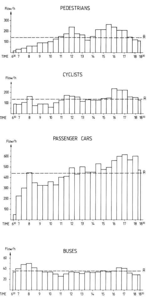
presen-ted in figure 2. In figure 3 the estimapresen-ted hourly flow is presenpresen-ted for
passenger cars, buses, bicyclists and pedestrians.
In figure 2 it can be seen that the proportion of bicycles and buses is relatively high during the morning hours.
The proportion of pedestrians increases during morning and early mid-day
and reaches maxima about 12 and 15 16.
°/o l 100 % flow/h Pedestrians 18,1 1&1 90
-80
Cyclists
17,2 134
70 " :§:;:;:5 Motorcyclists133 :::: 153515 :'Ä'I' .. :-:-:-:- ":? (MODQÖFid ers 1,9 110
60 - 515321; 53533: Efåfäfåfgzgzgzg .. g Buses 4,6 36
w awn
ma...%&
uma
w M
50 . 53:36:53. ' 40 -5555 Passenger cars 56,3 438
30-
100 777
20 -10 ,TIME 630 7 8 9 10 11 12 13 11» 15 16 17 18 1830
Figure 2. Traffic composition in the central part of Linköping,
Figure 3. Flovn/h PEDESTRIA NS
mo-zoo:
*
1002
_
""""me '"
" m rl
TIME 630 7 8 9 10 11 12 13 1L 15 16 17 How/h CYCLISTS
10 11 12 13 1Å 15 16 17 18 1830 PASSENGER CARS Flow/h 11
mi
rT_n
500 - r- FT "_ __ F "V _ _u- -_=- ___-_,- - -__ __ __ __ __ -+ M 400 _a l 300- 200-100 ~_ . _. _. _. TIME 630 7 8 9 10 11 12 13 % 15 16 17 18 1830 Flow/h BUSES 60- A0-20
TIME 630 7 8 9
Estimated flow/h for pedestrians, cyclists, passenger cars and buses in the central part of Linköping.
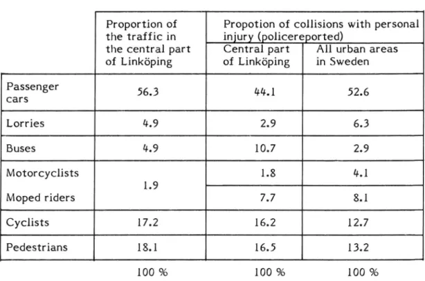
As we now have an estimate of the prOportions of different road user
groups, it can be of some interest to investigate the corresponding
appearance in police reported accidents concerning collisions with perso-nal injuries. We also present this figures for all urban areas in Sweden (table 1).
Buses, pedestrians and cyclists are over-represented in the central part of
Linköping a business, service and administration centre for about
100.000 persons - compared with all urban areas in Sweden.
Table 1. The prOportions of different vehicle or road user groups in
Linköping and the corresponding appearance in police
repor-ted accidents in Linköping and all urban areas in Sweden.
Proportion of PrOpotion of collisions with personal
the traffic in injury (policereported)
the central part Central part All urban areas
of Linköping of Linköping in Sweden
Passenger
56.3
44.1
52.6
cars Lorries 4.9 2.9 6.3 Buses 4.9 10.7 2.9 Motorcyclists 1.8 4.1 1.9 MOped riders 7.7 8.1 Cyclists 17.2 16.2 12.7 Pedestrians 18.1 16.5 13.2 100% 100% 100%Pedestrian safety. Relationship between degree of separation and traffic
flow.
The measurements of the degree of separation for pedestrians show that
the degree of separation is independent of the pedestrian flow but is by
definition negatively correlated with the motor vehicle flow.
The choice of measurement method has a theoretical background based on the fact that pedestrians and motor vehicles are arriving at the pedestrian crossing with a constant probability in time. Time appearance for cars on the pedestrian crossing is A seconds, and B seconds for the pedestrians passing the pedestrian crossing. The theoretical degree of separation the
becomes:
_ Motorvehicle flow/h ~ (A+B)
ST = 1
3600
This means that the theoretical degree of separation is decided by the
product of motor vehicle flow and the sum of the average passing times
across the pedestrian crossing for motor vehicles and pedestrians.
If it is a signalized intersection only the left and right turning traffic is
treated and only the period of green light for pedestrians. The theoretical
degree of separation can then be calculated as:
ST _ 1 Left and right turning motorvehicle flow/h- (A+B)
'
x
X : number of seconds per hour when both pedestrians and motor
vehicles have green phase.
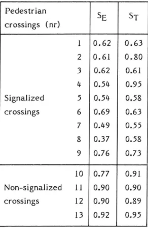
Both the theoretical (ST) and empirical (SE) degree of separation are calculated for 13 pedestrian crossings (table 2).
The figures mean that if the degree of separation is 0.90, 90 % of all pedestrians can pass the street without disturbing or being disturbed by
motor vehicles. Passage time for motor vehicles has not been accounted
for in the calculation of the theoretical degree of separation for the crossings. The passage time for the pedestrians was assumed to be # or 5
Table 2. Emperical (SE) and theoretical (ST) degree of separations
from motor vehicles for pedestrians on pedestrian crossings. - Signalized and non-signalized crossings.
Pedestrian SE ST crossings (nr) 1 0. 62 0.63 2 0.61 0.80 3 0.62 0.61 4 0.54 0.95 Signalized 5 0.54 0.58 crossings 6 0.69 0.63 7 0.49 0.55 8 0.37 0.58 9 0.76 0.73 10 0.77 0.91 Non-signalized 11 0.90 0.90 crossings 12 0.90 0.89 13 0.92 0.95
The empirical observations can also give different measurements of the degree of separation for pedestrians crossing the street depending on
directions and lane.
Relationship between collisionZ risk and flow
A model close at hand for predicting the number of collisions between
pedestrians and motor vehicles is a multiplicative model with pedestrian
and motor vehicle flow as predictors. One such regression model was
tested on police reported collisions between pedestrians and motor vehicles, which had occured during daytime in central Linköping during the last five years. For this, the daytime period was divided into six two-hour periods. The result indicates an increase in the number of collisions
both with increasing pedestrian flow and increasing motor vehicles flow (figure 4).
COLLlSIONS (C) BETWEEN
MOTORVEHICLES (M) AND
PEDESTRIANS (P)
ll
EMP MOdEl: dCMF za Pb M
600 M/h
R2 : 0,76
500 M/h
400 M/h
/
_ 300 M/h
/
4 zoo M/h
100
200
300
P/ h
Figure #. Calculated relationships between collisions and pedestrian
flow for different motor vehicle flow.
A possible risk measurement for pedestrians crossing street is
r _ Number of collisions between pedestrians and motor vehicles _ CMP
p Number of pedestrians crossing the street P
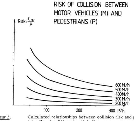
When the predicted number of collisions according to the regression model is used in the expression for risk, the following relation is obtained for different pedestrian flows (figure 5). The risk increases with increasing motor vehicle flow and it increases with decreasing pedestrian flow at a
RISK OF COLLISION BETWEEN
MOTOR VEHICLES (M) AND
.
C
» Risk ge
PEDESTRIANS (P)
500M/h
hOOM/h
.
.
'
'
. zoom/h
100
200
300 P/h
Figur 5. Calculated relationships between collision risk and
pedes-trian flow for different vehicle flow.
Relationship between collision, risk and degree or separation
As we have seen above a great part of the pedestrians are separated from
the motor vehicle traffic and therefore of no value for explaining the
probability of collison. This also means that it is better to use the number of non separated pedestrians than the total pedestrian flow, as a predictor
for the number of collisions.
If the number of non separated pedestrians is used as a predictor in the regression model, the degree of explanation becomes somewhat higher (0.81) i.e. somewhat stronger relationship (correlation 0.9), than if the total number of pedestrians is used. The character of the relation does not change. In these results the degree of separation has been calculated from three randomly chosen 5 minute periods of every observation period. Another risk measurement can be defined, in which the denominator consists of those pedestrians who are not separated from the motor
10
The number of collisions can be estimated according to the definition of
risk with the following espression:
c
MP : r15'
P - (1-5)The number of collisions then becomes a function of risk, pedestrian flow and degree of separation.
The material used here indicates that risk (ré) and pedestrian flow are
independent. This means that for a certain degree of separation, the risk is constant for varying pedestrian flow. The number of collisions will at a certain degree of separation increase or decrease proportionally with the pedestrian flow.
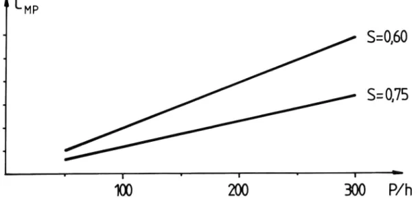
It has been possible to study the relation between number of collisions and
pedestrian flow for two degrees of separation 0.60 and 0.75 (figure 6).
The result shows that a change in degree of separation from 0.60 to 0.75 will lower the risk for collisions between pedestrian and motor vehicles 10% and decrease the number of collisions by %%
l CMP
-
S=O,6O
S= 0,75
160
'
260
'
360 åh
Figure 6. Calculated relationships between collisions and pedestrian
flow for two different values of the degree och separa-tion.
11
Conlusions
The aim of this paper is to point out some possibilities in order to evaluate the traffic situation in urban areas by quantitative estimation of the effectiveness of measures to increase the traffic safety situation for unprotected road users.