SSM’s external experts’ review of
SKB’s analysis of long-term safety of
1BMA (SFR)
SSM perspective
BackgroundFractures in the concrete barrier of the rock vault 1BMA in the final
repository for low and intermediate level waste (SFR) have been
observed. The Swedish Radiation Safety Authority (SSM) enforced
Swedish Nuclear Fuel and Waste Management Company (SKB) to assess
the long-term radiological consequences of 1BMA (SSM2015-2432-26)
given the present state of the rock vault concrete barrier and feasible
reinforcement scenarios.
The present report presents the results from SSM’s external experts’
review of SKB’s responses and analyses to address the enforcement
notice from SSM. SKB’s analyses demonstrate long-term consequences
of leaving the concrete barrier in the rock vault 1BMA in SFR without
repair, alternatively partially repairing the concrete walls. The general
objective of this project is to develop a basis for SSM’s own review of
SKB’s analyses (SSM2015-2432-34).
Project information
Contact person SSM: Henrik Öberg
Reference: SSM2013-4854
Authors: Osvaldo Pensado1) and Biswajit Dasgupta1) 1) Southwest Research Institute, San Antonio, Texas, USA
Review of SKB’s analysis of
long-term safety of 1BMA
(SFR)
Activity number: 3030014-2004 Registration number: SSM2018-3264 Contact person at SSM: Henrik Öberg
This report concerns a study which has been conducted for the
Swedish Radiation Safety Authority, SSM. The conclusions and
view-points presented in the report are those of the author/authors and
do not necessarily coincide with those of the SSM.
Abstract
This report documents an evaluation of SKB responses and analyses to address an injunction by SSM regarding consequences of leaving concrete walls with existing fractures without repair in 1BMA, as well as consequences of partial reinforcement of concrete structures. SKB concluded that the dose of the Partial Reinforcement Case is similar to the mean annual effective dose of the SR-PSU Main Scenario. SKB computed moderate increases in dose estimates for the No-Repair Case. Those increases associated with 1BMA are minor in the context of the total SFR mean annual effective doses (including contributions from all disposal systems, not just 1BMA).
For this evaluation, a simplified COMSOL model was used to relate changes in water flux to the changes in hydraulic conductivity of components of the 1BMA system. It was concluded that changes in flow rates SKB computed associated with different cases of concrete hydraulic conductivity are reasonable. Although flow rates changed by one and two orders of magnitude (from the Main Scenario to the Partial Reinforcement Case and to the No-Repair Case), mean annual effective doses SKB computed increased only by a factor of 2 or 3. Such relatively minor increases are due, in part, to the relative contribution of diffusion to the radionuclide fluxes, especially when flow rates are low (i.e., radionuclide release rates are not
proportional to flow rates when flow rates are low).
SKB may not use grout in compartments with a dominant proportion of bituminized waste, as a strategy to address volume expansion of the water-saturated bitumen matrix. Based on the simplified COMSOL model, it was concluded that considering much higher hydraulic conductivity for compartments with bituminized waste (to simulate initial void space without grout) does not significantly increase water fluxes. Based on SKB sensitivity analyses, changes to radionuclide release rates and dose estimates in 1BMA are expected to be moderate if radionuclide sorption to grout in compartments with bituminized waste were disregarded. We recommend requesting SKB to quantify effects of disregarding radionuclide sorption to grout in compartments with bituminized waste.
We recommend requesting SKB to supplement the analysis of the effect of corrosion on the initial hydraulic conductivity of degraded concrete, to address SKB’s
conclusions (in the report R-13-40) regarding potential activation of steel corrosion by chloride. (According to R-13-40, critical chloride levels in concrete to activate corrosion may be attained in a few years to a few decades.) Various studies published elsewhere, however, consistently conclude that the rate of corrosion of carbon steel is independent of chloride concentration in anaerobic concrete porewaters. Thus, chloride activation may be feasible only during transient aerobic conditions after repository closure.
It is not clear why different mean annual effective doses are associated with the same cases [see Figure 1(c), Partial Reinforcement Case, and Figure 8, Main Scenario, in this report]. We recommend a clarification question to SKB to address this minor issue.
It is considered that questions identified in this report would not necessarily change the SKB conclusions that the existing fractures in 1BMA have only a minor effect on total SFR mean annual effective doses and the overall risk.
Contents
1 Introduction ... 1
2 SKB Analysis ... 2
2.1 Summary of the SKB response ... 2
2.2 Summary of SKB radionuclide release computations ... 3
3 Evaluation of SKB Results ... 8
3.1 Hydraulic conductivity ... 8
3.1.1 Effect of Steel Corrosion on the Hydraulic Conductivity of Concrete ... 9
3.1.2 Conclusions on Selection of Hydraulic Conductivity for Degraded Concrete Conditions ... 12
3.2 Flow Computations ... 13
3.3 Radionuclide Release Computations ... 18
4 Conclusions ... 22
5 References ... 25
1 Introduction
This report documents an independent review of SKB’s response to injunction SSM2015-2432-26 regarding post-closure safety of the 1BMA vault. The present state of 1BMA exhibits fractures in concrete walls. On the other hand, in the Main Scenario (global warming case denoted as CCM_GW) of the radionuclide release computations in the Radionuclide Transport Report TR-14-09, SKB assumed pristine or repaired concrete (i.e., fracture-free concrete). SSM prescribed an injunction requesting SKB to analyse the long-term consequences if only minor repairs were implemented on concrete structures. SKB replied to the injunction with a document titled “Updated analysis of the post-closure radiation safety for 1BMA in SFR1—translation of SKBdoc 1686798,” Document ID 1697595, dated September 18, 2018. This report documents a review of the SKB response to the injunction and an evaluation of the updated radionuclide release computations and dose estimates. The review is developed in Sections 2 and 3. Section 2 includes a summary of the SKB response to the injunction, and of the radionuclide release computations supporting the response. Section 3 presents the evaluation of the response, focusing on the effective hydraulic conductivity of concrete, water flow computations, and radionuclide release computations. Conclusions are presented in Section 4. Section 5 is the list of references. An appendix lists the SKB documents covered in this report.
2 SKB Analysis
2.1 Summary of the SKB response
SKB identified the presence of penetrating fractures in 1BMA with apertures in the range of 0.1 to 1 mm. SKB stated that the main cause of those fractures was temperature shrinkage during construction. Accordingly, SKB refers to those fractures as “temperature fractures” to differentiate from other fractures arising from chemical alteration and dissolution. SKB estimated the effective hydraulic
conductivity of the concrete walls with heavy fracturing to be in the range 10−5 to 10−4 m/s, disregarding any flow resistance in the waste domain.
SKB examined steel form rods on the concrete and fracturing arising from corrosion of those form rods in 1BMA. Carbon steel passively corrodes in alkaline and anoxic concrete porewater. Iron corrosion products occupy more volume than the original metal, and can cause the concrete to crack. Considering corrosion rates
representative of carbon steel in alkaline anoxic conditions (50 nm/yr, from Table 5-3 of TR-14-10), SKB estimated relatively small fracture apertures and minor increases in the effective hydraulic conductivity during the first 2,000 years. After 10,000 years, fractures arising from the corrosion product volume expansion may be of comparable aperture to the current fractures. Form rods would corrode 0.5 mm in 10,000 years, out of an initial diameter of 12 mm. SKB asserted that the remaining metal in the form rod cavities and remaining corrosion products (in the cavities and deposited in the fractures) will offer resistance to flow; the effective hydraulic conductivity of the concrete structure is expected to remain below 10−5 m/s.
SKB concluded that considering a hydraulic conductivity equal to 10−5 m/s to represent the current state of concrete walls in the 1BMA system (moderately degraded concrete) is reasonable. SKB also concluded that no corrections to the hydraulic conductivity are needed to account for additional fractures and form rod cavities caused by corrosion of steel form rods in the first 10,000 years. SKB concluded that other processes such as chemical dissolution and rockfall are not expected to affect the effective hydraulic conductivity in the first 20,000 years, based on geochemical modelling and assessments of rock and tunnel stability.
SKB implemented alternative radionuclide release and transport computations and concluded that enhanced flow rates (due to the presence of fractures in concrete walls) affect only to a relatively minor degree the radionuclide releases and dose estimates reported in the Radionuclide Transport and Dose Calculations Report TR-14-09.
2.2 Summary of SKB radionuclide release
computations
SKB implemented the following assumptions in the analyses.
No-Repair Case
The hydraulic conductivity, K, of the concrete (walls, lid, and base slab) of 1BMA equal to 10−5 m/s during the first 20,000 years, and increasing to 10−3 m/s afterwards
K for backfill equal to 10−3 m/s
K for waste form equal to 10−3 m/s (from Equation 3-1 in TR-13-08)
The effective concrete diffusivity and porosity were assumed consistent with the Accelerated Concrete Degradation case in TR-14-09
The partition coefficients (Kd) of the structural concrete were assumed equal to zero, based on the assumption of fast flow through fractures1
Partial Reinforcement Case
SKB considered the walls and lid reinforced with concrete, but the base slab would be left unrepaired.
K of concrete walls and lid initially equal to 10−7 m/s, increasing to 10−5 m/s at
20,000 years, and to 10−3 m/s at 52,000 years
K of base slab equal to 10−5 m/s, increasing to 10−3 m/s at 20,000 years
K for waste form initially equal to 10−4 m/s (from Equation 3-1 in TR-13-08),
increasing to 10−3 m/s at 20,000 years
The effective concrete diffusivity and porosity were assumed consistent with the Main Scenario (Climate Change Case) in TR-14-09
The Kd coefficients of the structural concrete were assumed consistent with the Main Scenario in TR-14-09 during the first 20,000 years, and then equal to 0 afterwards (based on the assumption fast flow through fractures)
SKB implemented computations of regional flow; corresponding results were used to define boundary conditions for a smaller-scale COMSOL model simulating the complete repository system, including 1BMA and a portion of the host rock domain. SKB accounted for different hydraulic conductivity values for multiple components in the system and computed steady-state flows. SKB computed average flow rates through the fifteen compartments of 1BMA using the COMSOL model. For each compartment, flow rates in the 𝑥, y, and z directions were computed to be used as input to radionuclide transport computations. Those flows are dependent on
hydraulic conductivities through structural concrete, waste form, and backfill region.
SKB used the Ecolego software for radionuclide transport computations. The radionuclide transport model relied on large control volumes to represent the concrete walls, lid, base slab, waste form, grout, and backfill region. A control volume was simulated as a perfectly-mixed system (without concentration gradients). Diffusive radionuclide transfer between adjacent control volumes is dependent on concentration differences, distances between centers of the control volumes, contact cross sections, diffusion coefficients, and porosities. Advective
1 According to Newson and Towler (2018), SKB also considered a flow splitting
approach, with 90 percent of the flow passing through open fractures and 10 percent of the flow passing through the concrete matrix, with the corresponding
mass transfer between adjacent control volumes depends on the flow rates computed in the COMSOL model, and radionuclide concentrations in those volumes. The SKB mass-balance computations accounted for equilibrium linear sorption (i.e., Kd approach2). The materials for which SKB assumed sorption include concrete, grout,
the matrix of the cementitious waste, bentonite clays, and the host rock. SKB did not consider radionuclide sorption to the bitumen matrix of the bituminized waste (Saetre and Lindgren, 2017). The extent of radionuclide retention due to sorption depends on the total volume of solids (concrete, grout, cementitious materials, and bentonite). SKB did not present information regarding the volume of grout considered in the computations in any of the documents we consulted.
SKB developed inventory estimates depending on average waste package types, and the number of waste packages, for each of the fifteen compartments in 1BMA. Inventory estimates are documented in the Report R-13-37. A different inventory was assigned to each compartment of 1BMA. The Radionuclide Transport Report TR-14-09 summarizes the total initial inventory of 1BMA aggregated over the fifteen compartments.
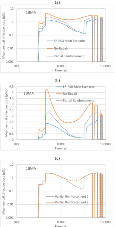
SKB used the existing Accelerated Concrete Degradation Case of the SR-PSU analysis (documented in the Radionuclide Transport Report TR-14-09) to provide information on the effect of No-Repair of 1BMA. In the injunction response document (SKB, 2018), SKB updated the radionuclide release and dose estimate computations to address the Partial Reinforcement Case. SKB results (mean annual effective dose) for the No-Repair Case and Partial Reinforcement Case for the 1BMA system are presented in Figure 1(a). The plot in Figure 1(b) presents the same information, but in log-linear scale, to visually amplify differences. SKB included two sets of mean annual effective dose estimates for the Partial
Reinforcement Case; Figure 1(c) compares the two sets of dose estimates for 1BMA reported in the injunction response (SKB, 2018). We recommend that SKB clarify the reason for the difference in mean annual dose of the same Partial Reinforcement Case [Figure 1(c)].
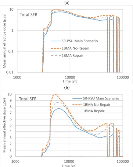
Figure 2 displays the total mean annual effective dose (dose estimates aggregated over all of the disposal systems—Silo, 1BMA, 1BLA, 1BTF, 2BTF, and so on) versus time for the SR-PSU Main Scenario, No-Repair of 1BMA, and 1BMA Partial Reinforcement cases computed by SKB. Data for Figure 2 were digitized from the SKB reports. Figure 2(a) presents the dose estimates in log-log scale, as originally presented by SKB. Figure 2(b) presents the data in log-linear scales, to visually amplify differences.3
2 The radionuclide concentration per unit of volume of the solid matrix is assumed
proportional to the concentration in porewater. The proportionality constant equals
Kd times the solid density.
3 Some of sharp corners and inflections in Figure 2(b) may be merely artefacts of the
digitation approach. We gathered data by manual sampling with computer mouse clicks at discrete points of the SKB log-log curves.
(a)
(b)
(c)
Figure 1. Digitized data of mean annual effective dose reported by SKB for the 1BMA system. (a) SR-PSU Main Scenario (climate change) from Figure 5-5 of TR-14-09, No-Repair Case from Figure 5-6 of TR-14-09 (1BMA mean annual effective dose for Accelerated Concrete Degradation case), and Partial Reinforcement Case from Figure 5-5 of the injunction response (SKB, 2018). (b) Plot is equivalent to (a), but in log-linear scale. (c) SKB provided two different results for the Partial Reinforcement case in Figures 5-5 and 5-6 (SKB, 2018). 0.001 0.01 0.1 1 10 1000 10000 100000 Mean an n u al effectiv e d o se (m Sv ) Time (yr) 1BMA
SR-PSU Main Scenario No-Repair Partial Reinforcement 0 0.5 1 1.5 2 2.5 3 3.5 4 4.5 1000 10000 100000 M ean an n u al effec tiv e d o se (m Sv) Time (yr) 1BMA
SR-PSU Main Scenario No-Repair Partial Reinforcement 0.001 0.01 0.1 1 10 1000 10000 100000 M ean an n u al effec tiv e d o se (m Sv) Time (yr) 1BMA Partial Reinforcement 1 Partial Reinforcement 2
(a)
(b)
Figure 2. Digitized data of mean annual effective dose reported by SKB for the SFR (total over all disposal systems, including 1BMA), including the SR-PSU Main Scenario (climate change case), 1BMA No-Repair Case, and Partial Concrete Reinforcement (labelled “1BMA Repair”); (a) plot in log-log scale, (b) same plot in log-linear scale to visually amplify differences.
SKB explained that the dose estimates increased from the SR-PSU Main Scenario to the Partial Reinforcement Case because of increases in flow rates through the waste form. The Partial Reinforcement Case is very similar to the Main Scenario, but it differs in the assumption that the base slab is without repair. The hydraulic conductivity, K, of the base slab in the Partial Reinforcement Case was assumed to be higher than the concrete walls and concrete lid K (e.g., base slab K = 10–5 m/s from 2,000 to 22,000 years in the Partial Reinforcement Case, while base slab
K = 10–7 m/s in the Main Scenario). COMSOL computations output higher flow
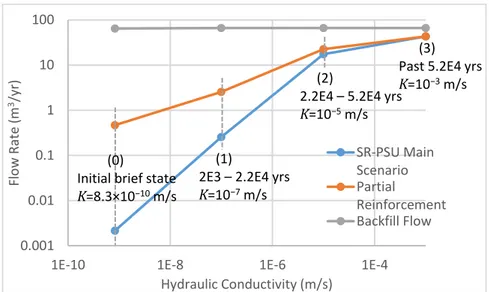
rates through waste forms in the Partial Reinforcement Case compared to the SR-PSU Main Scenario because of the higher hydraulic conductivity through the base slab in the former case. The computed flow rates are presented in Figure 3. The state indicated with a (0) is an initial state (concrete K=8.3×10⁻¹⁰ m/s), which SKB indicated to be relatively brief and not important to radionuclide transport
computations. The state labelled with (1), concrete K=10−7 m/s, was used to define flows from 2,000 to 22,000 years. The Partial Reinforcement Case flows are one order of magnitude higher than the SR-PSU Main Scenario; however, dose estimates are only less than a factor of 2 higher [Figure 1(b)]. SKB explained that dose
0.01 0.1 1 10 1000 10000 100000 M ean an n u al effec tiv e d o se (m Sv) Time (yr) Total SFR
SR-PSU Main Scenario 1BMA No-Repair 1BMA Repair 0 1 2 3 4 5 6 7 8 9 10 1000 10000 100000 M e an annual e ff e ct iv e do se ( mSv) Time (yr)
Total SFR SR-PSU Main Scenario
1BMA No-Repair 1BMA Repair
estimates increase by much less than one order of magnitude because diffusion significantly contributes to near-field radionuclide fluxes in 1BMA, and total radionuclide releases are not linearly proportional to flow rates (that is, radionuclide releases scale less than linearly with flow rates). The state (2) in Figure 3, concrete K = 10−5 m/s, was used to define flow rates in the period from 22,000 to 52,000 years. Full degradation of the engineered barrier system was assumed past 52,000 years. At that point [state (3) in Figure 3] the hydraulic conductivity of the concrete, base slab, waste form, and backfill was assumed to equal 10−3 m/s.
Figure 3. Flow rates SKB computed using a COMSOL model. The data source for this plot is Figure 5-3 of the injunction response document (SKB, 2018). Noted K values are for the Main Scenario, and for all concretes except the base slab in the Partial Reinforcement Scenario.
Dose estimates for the No-Repair Case are less than a factor of 2 greater than dose estimates of the Partial Reinforcement Case [Figure 1(b)]. SKB explained that the increase in the mean annual effective dose is due to (i) higher flows and (ii) neglect of sorption on concrete walls and concrete lid.
The effect of higher dose estimates for the No-Repair and Partial Reinforcement Cases was propagated to the SFR dose estimates (including contributions from all the disposal systems, such as Silo, 1BMA, 1BLA, 1BFT, and 2BFT). Dose estimates associated exclusively with 1BMA (Figure 1) propagate into minor changes (less than one order of magnitude increase) in the overall SFR mean annual effective dose (Figure 2). 0.001 0.01 0.1 1 10 100
1E-10 1E-8 1E-6 1E-4
Fl o w Rate (m 3/y r) Hydraulic Conductivity (m/s) SR-PSU Main Scenario Partial Reinforcement Backfill Flow (0) Initial brief state
K=8.3×10⁻¹⁰m/s
(1)
2E3 – 2.2E4 yrs
K=10−7m/s
(2)
2.2E4 – 5.2E4 yrs
K=10−5m/s
(3) Past 5.2E4 yrs
3 Evaluation of SKB Results
This evaluation focused on the following aspects: hydraulic conductivity of degraded concrete, flow computations, and dose estimates.
3.1 Hydraulic conductivity
SKB, in the injunction response report (SKB, 2018), presented two calculation cases for long-term radiological safety of the 1BMA vault. In one case SKB considered the current degraded stage of the construction concrete with existing fractures. In the second case SKB assumed new, externally reinforced concrete, 0.3-m thick outer walls and an additional 0.8-m thick lid, while keeping the base slab without repair. The hydraulic conductivity used for existing concrete is given in Table 4-1 and Figure 4-3 of the injunction response (SKB, 2018). For the No-Repair Case, the hydraulic conductivity for the initial 22,000 years was assumed equal to 10−5 m/s, and for 22,000 years to the performance period (100,000 years), 10−3 m/s. For the Partial Reinforcement Case, the initial state of hydraulic conductivity for the reinforced concrete was assumed equal to 8.3×10⁻¹⁰ m/s; the conductivity was then increased to 10−7 m/s (between 2,000 to 22,000 years), 10−5 m/s (between 22,000 and 52,000 years), and 10−3 m/s (from 52,000 to 100,000 years).
SKB evaluated the effects of fractures on the hydraulic conductivity of concrete in the 1BMA vaults (SKB, 2018). SKB attributed the existing fractures in the construction concrete to temperature changes and shrinkage. Inspection of the concrete structure in 1BMA revealed the formation of fractures on the floor and walls (SKB R-13-40 and SKB R-13-51). Some fractures extended through the walls and were visible from inside and outside of the wall. Although the 1BMA concrete walls have several steel bolts, fractures related to corrosion of bolts have not been observed (SKB R-13-40). Using the fracture information (i.e., length and width) collected at sections of the 1BMA concrete wall in 2000 and 2011, SKB calculated the fractured concrete hydraulic conductivity. Based on the data collected during the year 2000 (fractures of aperture ranging from 0.1 to 1 mm, SKB, 2018), the
estimated concrete hydraulic conductivity was 5.2×10⁻⁵ to 1.1×10⁻⁴ m/s for the western long side and 1.1×10⁻⁴ to 2.2×10⁻⁴ m/s for the eastern long side, and, with additional data collected from the entire vault during 2011, the concrete hydraulic conductivity was estimated equal to 2.6×10⁻⁴ to 5.3×10⁻⁴ m/s (SKB R-13-40, Section 6.15). The hydraulic conductivity SKB considered for degraded concrete (10−5 m/s) in the updated analysis is less than values computed by Höglund (ranging from 5.2×10⁻⁵ to 5.3×10⁻⁴ m/s in SKB R-13-40, Section 6.15).
The estimation of hydraulic conductivity in SKB R-13-40 is based on the
assumption that the flow in fully penetrating fractures behaves as ideal flow between two parallel plates, with computations including corrections for surface roughness of fracture faces (SKB R-13-40). The overall effective hydraulic conductivity estimate accounts for fractured concrete (using the measured fracture size and number of fractures) and unfractured or intact concrete (Equation 6-7 in SKB R-13-40). The hydraulic conductivity of intact concrete was assumed to be 10−11 m/s. The approach used by Höglund (SKB R-13-40) to estimate the hydraulic conductivity of concrete is technically sound, but will likely overestimate the hydraulic conductivity. For example, in the simplified models in SKB R-13-40 it was assumed that fracture
channels are perfectly aligned with the large-scale average flow direction. In reality, there is no correlation between the local fracture orientation and the large-scale average flow direction. If fracture orientations and connected fracture networks were accounted for, estimates of the effective hydraulic conductivity would be less than in SKB R-13-40. Another factor causing overestimation of the effective hydraulic conductivity is the assumed hydraulic conductivity of intact concrete (10−11 m/s), which is a high value. For example, El-Dieb and Hooton (1995) measured the hydraulic conductivity of concrete of low, medium, and high strength. Based on the mix proportion of structural concrete (Table 7-1, SKB TR-14-10), the concrete in SFR is similar to the medium strength concrete, and for this concrete type the hydraulic conductivity ranges from 3.72×10⁻¹⁴ to 2.83×10⁻¹³ m/s for ordinary, unfractured, concrete. The hydraulic conductivity of the intact concrete in the SKB calculations is at least two orders magnitude higher than experimental values by El-Dieb and Hooton (1995). The upper value computed in Section 6.15 of SKB R-13-40 for degraded concrete (5.3×10⁻⁴ m/s) has embedded assumptions intended to overestimate the effective hydraulic conductivity. Therefore, selecting 10−5 m/s as the hydraulic conductivity of degraded concrete is judged to be reasonable.
SKB also considered the effect of corrosion of the form rods in the concrete wall on the hydraulic conductivity (SKB, 2018). The 12-mm diameter steel rods embedded in the concrete may corrode and induce fractures in the concrete as a result of the volume expansion of iron corrosion products. However, based on the passive rate of corrosion of steel in alkaline porewaters, SKB concluded that effects of steel corrosion on the hydraulic conductivity after 2,000 years would be minimal. After 10,000 years the apertures of the fractures in concrete caused by the volume expansion of the steel corrosion products are estimated to be comparable to existing penetrating fractures. Therefore, SKB concluded that steel corrosion would not contribute to significantly enhance the initial hydraulic conductivity of fractured concrete. Based on detailed calculations (documented in SKB R-13-40), SKB concluded that as the form rods corrode and crack the concrete, the effective hydraulic conductivity of concrete is bounded by the conductivity of the initially fractured concrete.
3.1.1 Effect of Steel Corrosion on the Hydraulic
Conductivity of Concrete
A review of the SKB model to address fractures in concrete from corrosion of steel is briefly documented. Corrosion of form rods and rebar was evaluated in SKB R-13-40 in regards to potential effects on the hydraulic conductivity of concrete. A simplified geometry (an iron cylinder embedded in a co-axial cylindrical concrete shell) was considered in the report SKB R-13-40 to take advantage of available closed-form equations for stresses and elastic deformations. Cracks would form when the tangential stresses in the concrete arising from the volume expansion of corrosion products equals the tensile strength of concrete (1.5×10⁶ Pa in SKB
R-13-40). The SKB analysis concluded that corrosion of 0.34 mm along the radial direction of the steel cylinders would be sufficient to establish critical stress
conditions to initiate the development of cracks. It would take a few years to several decades for carbon steel under passive conditions to corrode 0.34 mm.
SKB concluded that the fracture aperture is more important than the number of fractures or fracture spacing to the overall hydraulic conductivity (e.g., R-13-40,
Figure 6-1). Accordingly, SKB estimated fracture apertures arising from cracking due to the volume expansion of steel corrosion products. SKB employed equations by Li et al. (2005, 2006) to compute the fracture aperture as a function of the
corrosion depth.4 SKB simplified the equations by Li et al. by assuming that the
corrosion depth was small compared to the diameter of the steel form rods. Based on stress balance and pre-existing cracks, the equations by Li et al. indicate that the crack aperture is proportional to the corrosion depth. The proportionality constant for the system of interest to SKB is in the range 1.54 to 2.56 (i.e., aperture = constant × corrosion depth, with constant in the range 1.54 – 2.56). A similar proportionality between fracture aperture and corrosion depth was presented by Thoft-Christensen (2005). The existing “temperature” fractures are of aperture 0.1 to 1 mm (SKB, 2018). A minimal equivalent corrosion depth to cause fractures of 0.1 mm aperture is estimated as
𝑏 =0.1 mm
2.56 = 0.04 mm
(1)
If the passive corrosion rate is on the order of 5×10⁻⁸ m/yr, it would take at least 800 years for passive corrosion to cause fractures comparable to the existing temperature fractures:
𝑡 = 0.04 × 10
−3m
5 × 10⁻⁸ m/yr = 800 yr
(2)
The estimate in Eq. (2) is based on passive corrosion rates, ignoring any potential chloride or carbonate activation of steel. To match apertures of 1 mm, it would take 8,000 years for corrosion to build sufficient corrosion products. From Figures 6-1 and 6-9 of R-13-40, the effective hydraulic conductivity of concrete with fractures with apertures on the order of 0.1 mm is less than 10−5 m/s. SKB presented a similar analysis to Eqs. (1) and (2), with reference to Figure 6-9 of R-13-40 (effect of tiny fractures around form rods on K), and concluded it would take 10,000 years for corrosion products to cause fractures of aperture 0.75 to 1.25 mm. Prior to that time, SKB concluded that the hydraulic conductivity is dominated by the initial
temperature fractures. We find these conclusions by SKB to be reasonable, and consistent with our back-of-the-envelope estimates. The SKB conclusion relies on stress balance calculations that consider a concrete-steel system of cylindrical geometry (Li et al., 2005, 2006). The SKB conclusion on timing depends on the magnitude of passive corrosion rates (~5×10⁻⁸ m/yr). However, the SKB
conclusions do not account for conclusions in Section 4.2 of SKB R-13-40 (Figure 4-7) regarding chloride initiation of steel corrosion. According to analyses in that SKB report, it would take only a few years to a few decades for chloride diffusing through concrete to attain critical levels that activate corrosion of carbon steel. Under aerobic conditions, corrosion rates could increase by a factor of 10 or even more in the presence of chloride (e.g., Cesen et al., 2014). Upon closure of the repository, the transition from aerobic to anaerobic conditions will likely be relatively rapid.
On the topic of corrosion rates of carbon steel, a broad range of values are reported in the literature. Corrosion rates vary with time; long-term techniques indicate decreasing rates with time, possibly due to formation of oxy-hydroxides that lower the reactivity of the metal surface. Passive corrosion rates for carbon steel are
4 The corrosion depth is defined as the propagation distance of the corrosion front
along the radial direction, measured with respect to the original surface of the steel cylinder.
consistently reported to be less than 0.1 mm/yr (e.g., Garcia-Diaz, 2010), especially in anaerobic conditions and waste disposal environments (Kurten et al., 2017; King and Watson, 2010; Senior et al., 2017; Smart et al., 2013 and 2017). The corrosion rate considered in SKB R-13-40, 5×10⁻⁸ m/yr, is consistent with passive corrosion rates for carbon steel in the literature, and with 20-year experiments sponsored by the Belgium radioactive waste disposal program (Smart et al., 2017). The steel passive state is promoted by the alkaline porewaters in the concrete, but can be altered by chloride and pH changes. The report SKB R-13-40 estimated that critical chloride levels would be attained in a few years to a few decades as a result of chloride diffusing into concrete from the groundwater (SKB R-13-40, Figure 4-7). In theory, chloride may promote depassivation, causing carbon steel to exhibit relatively high corrosion rates (on the order of 1 mm/yr or even higher; e.g., Cesen et al. 2014), provided the corrosion potential exceeds the pitting potential. Under anaerobic conditions the corrosion potential is too low to exceed the pitting or repassivation potential (Senior et al., 2017). Several experiments by multiple authors consistently conclude that carbon steel corrosion rates are independent of chloride concentrations in concrete porewaters under anaerobic conditions (Kurten et al., 2017; King and Watson, 2010; Senior et al., 2017; Smart et al., 2013), even at chloride porewater concentrations up to 20,000 ppm and in long-term experiments (Smart et al., 2017).
Iron dissolution is electrochemically balanced by the reduction of water (e.g., Equation 4-7 in R-13-40), which causes hydrogen evolution. Thus, water diffusion, water saturation, and displacement of water by hydrogen gas may be factors also constraining steel corrosion rates. For example, Smart el at. (2013) showed that water availability limits corrosion rates. These researchers detected hydrogen evolution only in steel embedded in cement immersed in water; and when concrete was not immersed in water, the rate of hydrogen evolution was below detection limits —indicating that the carbon steel corrosion rate was negligibly low when the water supply was limited (Smart el at., 2013).
The response to the injunction document (SKB, 2018) concluded that corrosion would not significantly affect the initial state of concrete to the degree that further adjustments would be needed to the degraded concrete conductivity value of K=10−5 m/s. However, as previously stated, the SKB analysis disregarded conclusions in SKB R-13-40 related to chloride activation of steel and potentially enhanced corrosion rates. We recommend to request SKB to evaluate whether chloride activation of steel would change their conclusions, taking into account any transition from aerobic (oxic) conditions to anaerobic (anoxic) conditions.
SKB considered other scenarios that would affect the hydraulic conductivity of concrete, such as (i) formation of porous corrosion products around form rods, filling form-rod hole penetrations (e.g. Figure 6-3 in R-13-40, and Figure 3-1 in the injunction response document, SKB, 2018); (ii) formation of empty cylindrical channels by the dissolution of corrosion products (Figure 6-6 in R-13-40); and (iii) disturbed zones around form rods (Figure 6-9 in R-13-40) . Scenarios (i) and (iii) were concluded to have minor effects on the effective K. Scenario (ii) could have a major effect on the effective K, depending on the extent of corrosion product dissolution. However, dissolution of corrosion products leaving empty or partially empty through-wall holes appears to be an extreme scenario, especially in anoxic alkaline porewaters (where iron corrosion products are thermodynamically stable). SKB analysed a more realistic scenario of corrosion product build-up, with corrosion products remaining in place, and causing the concrete to fracture. We
consider the SKB assessment focusing on fractures arising from volume expansion of corrosion products to be reasonable.
3.1.2 Conclusions on Selection of Hydraulic
Conductivity for Degraded Concrete Conditions
We conclude that the use of K=10−5 m/s for structural concrete with fractures is reasonable. SKB did not consider other higher K values output by its analysis to represent a degraded state. Not using other higher values is justifiable on the basis of extreme conditions assumed in the simplified models that overestimate values of the effective K (e.g., assuming that the fracture orientation aligns with large-scale average flow direction and assuming relatively high values, 10−11 m/s, of the hydraulic conductivity of intact concrete). SKB concluded that K=10−5 m/s did not require any initial correction to account for corrosion of form rods. However, SKB’s conclusion relied on the very low passive corrosion of steel (5×10⁻⁸ m/yr) and dismissed SKB’s own conclusions that steel corrosion might be activated by chloride in few decades. We still consider the selection of K=10−5 m/s to represent degraded concrete to be reasonable. For example, corrosion rates may becathodically constrained (by the availability of oxidants such as water), the corrosion potential would be too low to exceed the repassivation or pitting potential of the carbon steel under anaerobic conditions (Senior et al., 2017), and iron corrosion product build-up may slow down further corrosion. Various experiments in
deaerated concrete porewaters consistently indicate that carbon steel corrosion rates are independent of chloride concentrations (even at relatively high chloride
concentrations), and are less than −m/yr (Kurten et al., 2017; King and Watson, 2010; Senior et al., 2017; Smart et al., 2013 and 2017). However, there is a gap in the logic of the SKB analysis, and we recommend requesting SKB to supplement its analysis and address conclusions in R-13-40 regarding chloride-activated corrosion (e.g. Figure 4-7 in R-13-40), and transitory aerobic (oxic) states after repository closure.
For fully degraded concrete, we consider the SKB assumption of K=10−3 m/s—equal to the macadam backfill hydraulic conductivity—to be reasonable.
The hydraulic conductivity SKB assumed for reinforced concrete, discussed in Section 4.2.4 of the injunction response (SKB, 2018), is similar to values used in the modelling report on flow in the SFR 1 and SFR 3 systems (Table 6-2, SKB TR-13-08), where four sets of hydraulic properties were used: a base case (K=8.3×10⁻¹⁰ m/s), moderately degraded (K=10−7 m/s), severely degraded (K=10−5 m/s), and completely degraded (K=10−3 m/s) cases. The SKB estimates for the initial value of hydraulic conductivity of construction concrete are based on the assumption that the hydraulic conductivity of intact concrete is 10−11 m/s, the concrete would be slightly fractured, and steel corrosion is very slow. SKB addressed chemical concrete degradation by reactive transport modelling accounting for leaching of cementitious materials from the concrete barrier. The chemical model was used to evaluate the evolution of the individual mineral volumes and porosity for 1BMA and 2BMA during 100,000 years. Based on reactive transport modelling, SKB computed evolving values of hydraulic conductivity from changes to porosity using a modified Kozeney-Carmen relation. A more detailed review of the concrete hydraulic conductivity was documented previously (Dasgupta, 2017).
The numerical analyses SKB developed to estimate effective values of the hydraulic conductivity are technically sound, albeit designed to overestimate K. For example, SKB assumed K=10−11 m/s for pristine concrete, when experiments in the literature indicate lower conductivities. Hydraulic conductivities for cementitious materials reported in the literature vary broadly, with values as low as 10−14 m/s (e.g., Schneider, Mallants, and Jacques, 2012), and are highly dependent on water saturation. Based on quantitative analyses SKB provided and information in the literature, we consider the values of 10−7 and 10−5 m/s to be reasonable to represent moderate and severe states of concrete degradation.
3.2 Flow Computations
To evaluate flow computations, we implemented an independent COMSOL model with a simplified representation of 1BMA. We considered a cuboid or regular box domain of host rock [Figure 4(a)], with fixed hydraulic head on two opposing faces of the box [left-most and right-most faces of the box in Figure 4(a); with heads equal to 10 m and −10 m, respectively, selected to force flow from left to right], and a no-flux boundary condition on remaining faces of the box. Inside the host rock, we drew a simplified representation of 1BMA with fourteen compartments
(compartment 15 was ignored because of its different geometry). The concrete walls and lid, concrete base slab, and waste form were represented as systems with independent hydraulic conductivities. The backfill region was modelled with control volumes with hydraulic conductivity K=10−3 m/s, wrapping around the fourteen compartments [blue region in Figure 4(b)]. COMSOL was used to compute water fluxes based on Darcy’s law (relating water flux to the pressure gradient), and to solve the steady-state water balance equation. The simplified model was developed not to reproduce SKB computations, but to gain insights on terms controlling water fluxes and effects of changes in assumed values of the hydraulic conductivity. The red line in Figure 4(c) is a centerline. Water fluxes reported later were computed along this line.
Examples of COMSOL results are presented in Figure 5. The lines in Figure 5 are streamlines. The red streamlines highlight flow intercepting the left face of the disposal system. As flow moves to the right, in this simulation the streamlines tend to cluster in the backfill region—a phenomenon referred to as “hydraulic caging.” In this particular simulation, the concrete wall K=10−7 m/s, the waste form K=10−4 m/s, and the base slab K and backfill K both were set equal to 10−3 m/s.
(a)
(b)
(c)
Figure 4. Domain of the COMSOL simulations. Hydraulic heads equal to 10 m and −10 m were imposed on the left-most and right-most faces of the box in (a). The blue region in (b) represents the backfill. Waste form water fluxes were computed along the red centerline in (c).
(a)
(b)
Figure 5. Example of results of the COMSOL simulations. The lines are
streamlines, indicating flow directions. The red streamlines intercept the left-most face of the disposal system. In this particular simulation, concrete wall K=10−7 m/s, waste form K=10−4 m/s, and the base slab K and backfill K both were set equal to 10−3 m/s.
Figure 6 shows the magnitude of the water flux along the waste form centerline [red line in Figure 4(c)] for different combinations of the hydraulic conductivity. Each “bump” in the curves is associated with a compartment of 1BMA. The Main Scenario was simulated with concrete K=10−7 m/s, waste form K=10−4 m/s, backfill
K=10−3 m/s, and host rock K=2×10⁻⁸ m/s. The Partial Reinforcement Case was
similar, with the exception of base slab K=10−5 m/s. Changing the hydraulic conductivity of the base slab did not significantly affect the magnitude of the flux. The magnitude of the flux decreased in some locations in the Partial Reinforcement Case, that is, the yellow curve lies in general below the grey curve), which may appear counterintuitive. The plot in Figure 6 shows fluxes only along the centerline. Those fluxes can be reduced when enhanced fluxes occur in the base slab, thus explaining why the yellow curve is below the grey curve at some locations. The main conclusion in comparing the Main Scenario and Partial Reinforcement Case is that fluxes along the centerline are affected to only a minor extent by the increase in base slab K. The SKB results for waste form water flows indicate a change by a factor of 10 when the base slab K increased from 10−7 to 10−5 m/s [Figure 3, label (1)]. The SKB results are reasonable, taking into consideration different boundary conditions imposed by the regional model for water flow, and heterogeneity in the host rock hydraulic conductivity accounted for in the SKB model.
Figure 6. Water flux magnitude along the waste form centerline [red line in Figure 4(c)] for various cases of hydraulic conductivity combinations. Each bump in the curves is associated with a compartment of 1BMA.
SKB computed volumetric flows along six different directions for each waste compartment. Each flow rate was, most likely, computed by SKB by integrating the water flux projected along the normal direction of the six faces of each waste compartment. SKB was not specific with regard to what was represented by the flow rate in Figure 5-3 (SKB, 2018, Figure 3 in this report) (Is it an average flow over all directions and all compartments? Is it a maximum flow? What is the relationship of the flow to radionuclide transport computations?) Nonetheless, we consider a factor of 10 change in flow by changing the base slab hydraulic conductivity from 10−7 to 10−5 m/s [Figure 3, label (1)] to be reasonable.
0.001 0.01 0.1 1 0 20 40 60 80 100 W at er Flu x M ag ni tude (m/ yr ) Position (m) Main Scenario Partial Reinforcement No-Repair Fully Degraded
In the SKB Main Scenario computation (Figure 3), the flow rate increased by almost two orders of magnitude when the concrete hydraulic conductivity increased from 10−7 to 10−5 m/s. In the Partial Reinforcement Case, the increase in flow was only approximately a factor of 10. Those changes are comparable to changes from the Partial Reinforcement flux curve to the No-Repair flux curve in the new
computations shown in Figure 6. In the No-Repair Case, we assumed concrete K = 10−5 m/s, and waste form K = base slab K = 10−3 m/s (other hydraulic conductivities were the same as the Partial Reinforcement Case). The maximum change in the magnitude was approximately a factor of 30 between these two cases. As previously stated, the intention was not reproducing the SKB computations, but to obtain some insight into the potential flow response in 1BMA to changes in hydraulic
conductivity.
Finally, the increase in flow in both the Main Scenario and Partial Reinforcement curves in Figure 3 was approximately a factor of two when the concrete hydraulic conductivity increased from 10−5 to 10−3 m/s. Such increase is comparable to the increase in flux from the No-Repair Case to the Fully Degraded Case in Figure 6. In this latter case, we assumed K = 10−3 m/s for the concrete walls, concrete lid, base slab, and waste form.
SSM staff had expressed a concern regarding whether flows would be affected by the initial presence of void space in compartments with bituminized waste. The bitumen matrix will expand when saturated with water. A strategy to accommodate the expected volume expansion could be to not apply any grout backfill before closing the compartments with the bituminized waste. SKB accounted for lower flow resistance through the waste form by assuming waste form K = 1000 × concrete
K (Equation 3-1 in TR-13-08), and capping waste form K to a maximum value of
10−3 m/s. This enhanced value of the hydraulic conductivity for the waste form is intended to account for average effects, including the presence of void space. When concrete K = 10−7 m/s, SKB assumed waste form K = 10−4 m/s. Initially, waste containers and waste forms are of very low permeability, and a value such as
K = 10−4 m/s is expected to overestimate the effective hydraulic conductivity of the
waste container/waste form/grout/void space system. To help evaluate the potential effects of high hydraulic conductivity in bituminized waste compartments, we conducted a sensitivity analysis of our No-Repair computation by assuming a very high value of K (=1 m/s) for compartments dominated by bituminized waste (compartments 2, 3, 5, and 6 in 1BMA according to Table 3-14 in the Initial State Report TR-14-02). Using the simplified COMSOL model, the magnitude of the flux along the waste centerline changes by a moderate extent despite the very large of K assumed for compartments 2, 3, 5, and 6 (Figure 7). We conclude it is unlikely that the more detailed SKB model will produce significantly higher flows if void space were explicitly modelled. We judge it appropriate to derive flow estimates with the assumption that waste form K = 1000 × concrete K (SKB, 2013).
In summary, we judge technically appropriate the approach SKB implemented to compute flow rates and the simplifying assumptions, such as assuming the hydraulic conductivity of the waste is a factor of 1000 higher than the conductivity of
concrete. The response SKB provided to the injunction, computing flow rates for the No-Repair and the Partial Reinforcement Cases, accounts for the effect of thermal fractures on the hydraulic conductivity of concrete. The SKB analysis for the Partial Reinforcement Case yielded higher flows than the SR-PSU Main Scenario because of the higher hydraulic conductivity of the concrete base slab in the former case. The higher flows partially explain the slightly higher radionuclide release rate estimates
documented in the SKB injunction response. Additional evaluation of the radionuclide release computations is documented in the following section.
Figure 7. Water flux magnitude along the waste form centerline [red line in Figure 4(c)] for the No-Repair case with two variants. The No-Repair Case is the same as in Figure 6. In No-Repair 2, it was assumed waste form K = 1 m/s for 1BMA compartments 2, 3, 5, and 6. Each bump in the curves is associated with a compartment of 1BMA.
3.3 Radionuclide Release Computations
SKB computed higher dose estimates by a factor 1.6 (Table 4-4 of the injunction response, SKB, 2018) for the Partial Reinforcement Case compared to the SR-PSU Main Scenario (Figure 1). The increase in dose estimates is entirely attributable to the higher flow rates. Although SKB presented flows that are approximately a factor of 10 higher [Figure 3 label (1)], it is not clear whether SKB used those precise flow rates in the radionuclide transport computations. According to the SKB description, the radionuclide release and transport computations require flow rates along six directions, normal to the faces of the waste compartments, for each of the fifteen compartments in 1BMA. The flows in Figure 3 may be maximal values, and not necessarily used in the radionuclide transport computations. SKB stated that dose estimates differ by less than a factor of 10, because radionuclide releases are not linearly proportional to flow rates, in the regime of the Main Scenario. This assessment by SKB is reasonable. The following back-of-the-envelope computation is provided to compare transport by diffusion to transport by advection. If Q is a flow rate, A a cross section, and L a pathway distance, the liquid residence time, tL, is computed as 𝑡𝐿= 𝐿 𝑄/𝐴 = 𝐿 𝐴 𝑄 (3)
The travel time by diffusion along the same pathway distance L can be estimated as 0.05 0.1 0.15 0.2 0.25 0.3 0 20 40 60 80 100 W at er Flu x M ag ni tude (m/ yr ) Position (m) No-Repair No-Repair 2
𝑡𝐷 =
𝐿2
𝐷
(4)
where D is the diffusion coefficient. The Peclet number is defined as tD/tL: 𝑃𝑒 =𝑡𝐷 𝑡𝐿 = 𝐿 2/𝐷 𝐿 𝐴/𝑄 = 𝐿 𝑄 𝐷 𝐴= 𝐿 𝑣 𝐷 (5)
where 𝑣 is the liquid velocity. Advection dominates radionuclide releases when tL << tD (i.e., the liquid residence time is much shorter than the travel time by diffusion) or Pe >> 1. Conversely, if Pe << 1, then diffusion dominates the radionuclide releases. From Figure 4-2 of the injunction response document, a reference cross section A can be defined as 15.6 m × 8.9 m = 138.84 m2.
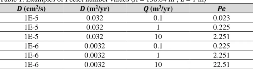
For diffusion coefficients on the order of 10−5 cm2/s, Peclet numbers in Table 1
indicate that radionuclide releases are dominated by advection when flow rates are on the order of 10 m3/yr. For diffusion coefficients on the order of 10−6 cm2/s,
radionuclide releases may be dominated by advection when flow rates are on the order of 1 m3/yr. For example, according to Figure 3 flow rates for the SR-PSU
Main Scenario are initially on the order of 0.1 m3/yr [label (1) in Figure 3], and
radionuclide releases are more likely dominated by diffusion. In the Partial Reinforcement Case, the flow rate is on the order of 1 m3/yr, and diffusion and
advection would both contribute to the radionuclide release rates. Although flow rates changed by one order of magnitude from the Main Scenario to the Partial Reinforcement Case [label (1) in Figure 3], radionuclide release rates and dose estimates are expected to increase by less than a factor of 10 (because release rates are not necessarily dominated by advection). In the injunction response document, SKB indicated that peak doses increased from 1.4 to 2.2 mSv/yr for the 1BMA system (Table 4-4, SKB, 2018); such increase is judged to be reasonable. SKB provided the flow rates documented in Figure 3 to develop a notion of overall changes when accounting for a degraded base slab, but SKB possibly used different flow rates from those in Figure 3 for the actual radionuclide release computations.
Table 1. Examples of Peclet number values (A = 138.84 m2, L = 1 m)
D (cm2/s) D (m2/yr) Q (m3/yr) Pe 1E-5 0.032 0.1 0.023 1E-5 0.032 1 0.225 1E-5 0.032 10 2.251 1E-6 0.0032 0.1 0.225 1E-6 0.0032 1 2.251 1E-6 0.0032 10 22.51
For the case of 1BMA without repair, SKB assumed an initial hydraulic
conductivity of the concrete of 10−5 m/s. From Figure 3, label (2), the initial flow rate for that case is approximately 23 m3/yr, which is almost two orders of
magnitude greater than the initial flow in the Main Scenario. SKB computed a peak dose equal to 4.2 mSv/yr for the No-Repair Case, which is only a factor of 3 greater than the Main Scenario peak dose (Table 4-2, SKB, 2018). As explained in the previous paragraph, the increase in the dose estimate is not necessarily linearly related to the increase in flow rates. In addition, detailed actual flow rates used in the radionuclide release and dose computations are not provided in SKB documents. Actual flow rates may differ by less than two orders of magnitude. Those two factors may be sufficient to explain why the peak dose estimates increased only by a factor of 3 from the Main Scenario to the No-Repair Case.
Overall, SKB radionuclide release and dose estimate computations are reasonable, but a few items need some clarification. The SKB computations take credit for radionuclide sorption to cementitious materials and bentonite clay (e.g., Tables 4-4 and 4-11 of TR-14-09). It is unclear how much sorption to grout contributes to limiting radionuclide releases, especially in compartments of 1BMA where bituminized waste is dominant. Backfill grout may not be applied to compartments with a dominant proportion of bituminized waste in 1BMA, as a potential strategy to accommodate for volume expansion of water-saturated bitumen. In the previous section it was concluded that assuming an average hydraulic conductivity between 10−4 and 10−3 m/s for the waste matrix/waste package/grout/void space system may overestimate flows to be input to radionuclide release and transport computations. Explicit representation of void space for a limited number of compartments (e.g., compartments 2, 3, 5, and 6 with a dominant proportion of bituminized waste) is not expected to significantly increase water flow rate estimates (for example see Figure 7). However, it is unclear whether SKB assumed backfill grout to be present in compartments with bituminized waste. If it did, computations may need to be revised to avoid taking credit for radionuclide sorption in grout if grout will not be used in some compartments.
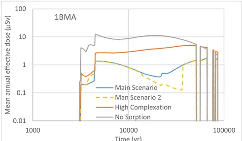
Changes of dose estimates can be inferred from sensitivity analyses in the Radionuclide Transport and Dose Calculations Report TR-14-09. The following Figure 8 includes 1BMA dose estimates for the Main Scenario (TR-14-09 Figures 5-5 and 5-5-7), the High Concentration of Complexing Agents Calculation Case (TR-14-09 Figure 6-42), and the No Sorption Case (TR-14-(TR-14-09 Figure 7-3). In the High Concentration of Complexing Agents Calculation Case, retardation coefficients in cementitious materials were decreased by a factor of 10. Changes in the mean annual effective dose are roughly within one order of magnitude when comparing the Main Scenario and the No Sorption cases. Therefore, if computations in the Main Scenario account for radionuclide sorption in grout material, revised dose estimates would increase only by less than a factor of 10. It is difficult to predict without detailed simulations the combined effects on dose of (i) increases in flow rates in the 1BMA Partial Reinforcement Case and (ii) decreases in the extent of radionuclide sorption in grout material. However, the information in Figure 1 and Figure 8 suggests that expected increases in the mean annual effective dose would be constrained in 1BMA (i.e., combined increases may amount to less than a factor of 10), and would have a small effect on the total SFR dose estimates. Nonetheless, we recommend to request SKB to address the effect on dose estimates of non-use of grout in compartments with a dominant proportion of bituminized waste.
In addition, SKB should clarify the reason for two different sets of mean annual effective dose for 1BMA [blue and yellow dashed curves in Figure 8 for the Main Scenario, and the two curves in Figure 1(c) for the Partial Reinforcement Case]. It appears that SKB applied some smoothing between 13,000 and 37,000 years, but we have not found any mention of smoothing in the SKB documents. Although the apparent smoothing does not affect peak dose estimates and the overall SKB conclusions, a technical basis is pertinent to avoid confusion.
Figure 8. Effect of retardation on 1BMA dose estimates. All data were digitized from plots in TR-14-09, specifically Main Scenario from Figure 5-5, Main Scenario 2 from Figure 5-7, High Concentration of Complexing Agents Case from Figure 6-42, and No Sorption Case from Figure 7-3.
It should be noted that SKB performed radionuclide transport computations using large control volumes in Ecolego (control volumes are finite elements of uniform concentration). Using large finite elements is known to be associated with large numerical dispersion, which tends to overestimate mass transfer rates among the control volumes, and overestimate radionuclide release rates, compared to approaches with very small finite elements. Also, the SKB model includes other features that tend to overestimate the radionuclide release rates, such as assuming limited resistance to water flow by waste forms and waste containers, and ignoring radionuclide sorption to concrete walls when concrete walls are fractured. However, it is difficult to assess whether assumptions, simplifications, and numerical methods overestimating releases would overcome aspects that underestimate releases (such as potentially taking credit for sorption to grout in compartments with limited volumes of grout). 0.01 0.1 1 10 100 1000 10000 100000 M ean an n u al effec tiv e d o se (m Sv) Time (yr)
1BMA
Main Scenario Man Scenario 2 High Complexation No Sorption4 Conclusions
SKB addressed the question posed by the SSM injunction by evaluating the consequences of leaving concrete walls with existing fractures without repair in 1BMA, as well as the consequences of partial reinforcement of concrete structures. SKB concluded that dose estimates for the Partial Reinforcement Case are similar to and only slightly higher than mean annual effective doses of the SR-PSU Main Scenario (peak doses differ by less than a factor of 2). The minor increases are associated with enhanced flow rates due to the presence of fractures in concrete base slabs, which would not be repaired. Moderate increases in dose estimates were computed for the No-Repair Case (peak doses differ by a factor of 3 with respect to the Main Scenario). The increases are associated with enhanced flows through fractured concrete and the absence of radionuclide sorption to concrete walls with fractures. Those increases associated with 1BMA become minor in the context of the total SFR mean annual effective doses, which include contributions from all disposal systems.
We used a simplified COMSOL model to evaluate changes in water flux resulting from changes in hydraulic conductivity. The simplified computations indicate that the macadam backfill would be an effective “hydraulic cage,” with flow occurring predominantly in this region of relatively high hydraulic conductivity. The simplified COMSOL model exhibited less sensitivity to changes in hydraulic conductivity than the SKB model. We concluded that the changes in flow rates SKB attributed to different selections of the hydraulic conductivity of the concrete are reasonable. Although flow rates changed by one and two orders of magnitude (from the Main Scenario to the Partial Reinforcement Case and to the No-Repair Case) in the SKB computations, mean annual effective doses increased only by a factor of 2 or 3. Such relatively minor increases are due, in part, to the relative contribution of diffusion to the radionuclide fluxes. Flow rates are very low, and diffusion is an important contributor and can even dominate the radionuclide fluxes. It is unclear how SKB used the computed flows (reported in Figure 3 in this report) in the actual radionuclide release and transport computations. SKB may have used different flow rates in its radionuclide release computations, also contributing to the apparent limited increases in release rates and dose estimates relative to changes in flow.
SKB may not use grout in compartments with a dominant proportion of bituminized waste, as a strategy to address volume expansion of the water-saturated bitumen matrix. Using a simplified COMSOL model we concluded that considering much higher hydraulic conductivity for compartments with bituminized waste (to emulate initial void space without grout) does not significantly increase water fluxes. Based on the results of sensitivity analyses in TR-14-09, we concluded that changes to release rates and dose estimates in 1BMA would be moderate if radionuclide sorption to grout in compartments with bituminized waste were disregarded. However, we recommend requesting SKB to more precisely quantify effects of disregarding grout sorption in compartments with bituminized waste (if SKB has not already dismissed such sorption).
We recommend seeking a clarification on reasons for reporting different mean annual effective doses for the same cases in the TR-14-09 and the injunction response document [see Figure 1(c) and Figure 8 in this report].
We recommend requesting SKB to supplement the analysis regarding the effect of corrosion on the initial hydraulic conductivity of degraded concrete (K=10−5 m/s), and to address conclusions in the report R-13-40 (e.g., Figure 4-7) regarding chloride activation of steel corrosion. (According to R-13-40, critical chloride levels in concrete to activate corrosion may be attained in a few years to a few decades.) The corrosion rate of depassivated steel may be, in theory, much higher than the assumed passive corrosion rate (5×10⁻⁸ m/yr). However, various studies consistently conclude that the rate of corrosion of carbon steel is independent of chloride
concentration in anaerobic concrete porewaters, and less than 10−7 m/yr (e.g., Kurten et al., 2017; King and Watson, 2010; Senior et al., 2017; Smart et al., 2013 and 2017). Thus, chloride activation may be feasible only during transient aerobic conditions after repository closure.
It is considered that questions identified in this document would not necessarily change the SKB conclusions that the existing fractures in 1BMA have only a minor effect on total SFR mean annual effective doses and the overall risk.
5 Acknowledgement
Dr. Stuart Stothoff (SwRI) helped with implementing the COMSOL model. Dr. David Pickett (SwRI) helped with technical and editorial review.
6 References
Cesen, A., T. Kosec, A. Legat, V. Bokan-Bosiljkov. 2014. "Corrosion Properties of Different Forms of Carbon Streel in Simulated Concrete Porewater." Materiali in tehnologije / Materials and technology, Vol. 48, No. 1, 2014, pp. 1–57.
Dasgupta, B. 2017. “Review of the hydraulic conductivity, Sorption, and
Mechanical Properties of Concrete Barriers of SFR-Main Review Phase.” Swedish Radiation Safety Autority (SSM): Stockholm, Sweden.
El-Dieb, A.S. and R.D. Hooton. 1995. “Water Permeability Measurement of High Performance Concrete Using a High Pressure Triaxial Cell”, Cement and Concrete Research, Vol. 25, No. 6, 1995, pp. 1199–1208.
Garcia-Diaz, B.L., 2010. “Life Estimation of High Level Waste Tank Steel for H-Tank Farm Closure Performance Assessment.” Report SRNL-STI-2010-00047. Savannah River National Laboratory (SRNL), Savannah River Nuclear Solutions: Aiken, South Carolina.
King, F. and S. Watson. 2010. "Review of the Corrosion Performance of Selected Metals as Canister Materials for UK Spent Fuel and/or HLW." Quintessa Report, QRS-1384J Version 2.1. "Appendix B Corrosion of Carbon Steel." Quintessa: Henley-on-Thames, Oxfordshire, United Kingdom.
https://rwm.nda.gov.uk/publication/review-of-the-corrosion-performance-of- selected-metals-as-canister-materials-for-uk-spent-fuel-and-or-hlw-appendix-b-carbon-steel/?download
Kursten, B., D.D. Macdonald, N.R. Smart and R. Gaggiano. 2017. "Corrosion issues of carbon steel radioactive waste packages exposed to cementitious materials with respect to the Belgian supercontainer concept." Corrosion Engineering, Science and Technology, Vol. 52, No. S1, 2017, pp. 11–16.
https://doi.org/10.1080/1478422X.2017.1292345
Li, C.Q., W. Lawanwisut, J.J. Zheng, and W. Kijawatworawet. 2005. “Crack Width Due to Corroded Bar in Reinforced Concrete Structures.” International Journal of Materials & Structural Reliability, Vol.3, No.2, September 2005, 87-94.
Li, C.Q., Robert E. Melchers, and Jian-Jun Zheng. 2006. “Analytical Model for Corrosion-Induced Crack Width in Reinforced Concrete Structures.” Structural Journal, Vol. 3, Issue 4, July 1, 2006, 479-487.
Newson, R., and G. Towler. 2018. “SR-PSU Main Review Phase: Further review of 1BMA and updated 2BMA design.” Swedish Radiation Safety Autority (SSM): Stockholm, Sweden. September 13, 2018.
Saetre P, Lindgren M. 2017. “Svar till SSM på begäran om komplettering av ansökan om utökad verksamhet vid SFR angående konsekvensanalys.” SKBdoc ID 1601415 ver 3.0, Svensk Kärnbränslehantering AB. (In Swedish.).
Schneider, S., D. Mallants, D. Jacques. 2012. “Determining hydraulic properties of concrete and mortar by inverse modelling.” Materials Research Society Symposium Proceedings, Vol. 1475, 2012.
Senior, N., R. Newman, S. Wang, and N. Diomidis. 2017. "Understanding and quantifying the anoxic corrosion of carbon steel in a Swiss L/ILW repository
environment." Corrosion Engineering, Science and Technology, Vol. 52:sup1, (2017) pp. 78-83, DOI: 10.1080/1478422X.2017.1303102
SKB. 2018. “Updated analysis of the post-closure radiation safety for 1BMA in SFR1 - translation of SKBdoc 1686798.” Document ID 1697595. Svensk Kärnbränslehantering AB (SKB, Swedish Nuclear Fuel and Waste Management Co.): Stockholm, Sweden. September 18, 2018.
SKB. 2015. “Radionuclide transport and dose calculations for the safety assessment SR-PSU.” Technical Report TR-14-09, Revised edition. Svensk
Kärnbränslehantering AB (SKB, Swedish Nuclear Fuel and Waste Management Co.): Stockholm, Sweden. October 2015.
SKB. 2014. “The impact of concrete degradation on the BMA barrier functions. Updated 2018-03.” Svensk Kärnbränslehantering AB (SKB, Swedish Nuclear Fuel and Waste Management Co.): Stockholm, Sweden. Originally published in 2014. SKB. 2014. “Data report for the safety assessment SR-PSU.” Technical Report TR-14-09. Svensk Kärnbränslehantering AB (SKB, Swedish Nuclear Fuel and Waste Management Co.): Stockholm, Sweden. November 2014.
SKB. 2014. “Initial state report for the safety assessment SR-PSU.” Technical Report TR-14-02. Svensk Kärnbränslehantering AB (SKB, Swedish Nuclear Fuel and Waste Management Co.): Stockholm, Sweden. November 2014.
SKB. 2013. “Flow modelling on the repository scale for the safety assessment SR-PSU.” Technical Report TR-13-08. Svensk Kärnbränslehantering AB (SKB, Swedish Nuclear Fuel and Waste Management Co.): Stockholm, Sweden. December 2013
SKB. 2013. “Låg- och medelaktivt avfall i SFR, Referensinventarium för avfall 2013.” Report R-13-37. Svensk Kärnbränslehantering AB (SKB, Swedish Nuclear Fuel and Waste Management Co.): Stockholm, Sweden. December 2013.
SKB. 2013. “Flow and transport in fractures in concrete walls in BMA - Problem formulation and scoping calculations.” Svensk Kärnbränslehantering AB (SKB, Swedish Nuclear Fuel and Waste Management Co.): Stockholm, Sweden. 2013. Smart, N.R., A.P. Rance, P.A.H. Fennell and B. Kursten. 2013. "The anaerobic corrosion of carbon steel in alkaline media –Phase 2 results." EPJ Web of Conferences, Vol. 56, 06003 (2013). DOI: 10.1051/epjconf/20135606003 Smart, N.R., A.P. Rance, D.J. Nixon, P.A.H. Fennell, B. Reddy, and B. Kursten. 2017. "Summary of studies on the anaerobic corrosion of carbon steel in alkaline media in support of the Belgian supercontainer concept." Corrosion Engineering, Science and Technology. Vol. 52:sup1, pp. 217-226, DOI:
10.1080/1478422X.2017.1356981
Thoft-Christensen, P., 2005. “Safety and corrosion cracking of concrete structures.” In Proceedings of 4th international workshop on life-cycle cost analysis and design of civil infrastructure systems, Cocoa Beach, Florida, 8–11 May 2005, 135–142. Villar, M.V., P.L. Martín, F.J. Romero, J.M. Barcala. 2012. “Results of the tests on concrete (Part 2).” FORGE Report D3.16. 45pp.
APPENDIX 1
Coverage of SKB reports
Following reports have been covered in the review.
Table A-1: List of reports consulted and evaluated in the task
Reviewed report Reviewed sections Comments SKB SKBdoc 1697595,
2018: Updated analysis of the post-closure radiation safety for 1BMA in SFR1 - translation of SKBdoc 1686798
All
SKB TR-14-02, 2014: Initial state report for the safety assessment SR-PSU
4, Appendix A Information of 1BMA compartments and distribution of bituminized and cementitious waste
SKB TR-14-09, 2015: Radionuclide transport and dose calculations for the safety assessment SR-PSU
4, 5, 6, 7, 9.3.3, Appendix D
SKB TR-14-10, 2014: Data report for the safety assessment SR-PSU
5, 6, 7
SKB TR-13-08, 2013: Flow modelling on the repository scale for the safety assessment SR-PSU
3 Equation 3-1 defines the hydraulic
conductivity assumed for the waste form. Table 6-2 defines hydraulic conductivities used in flow modelling SKB R-13-37, 2013: Låg-
och medelaktivt avfall i SFR, Referensinventarium för avfall 20
6 Description of average inventory per
waste package type
SKB R-13-40, 2014: The impact of concrete degradation
on the BMA barrier functions
2, 4, 5, 6, 7, 8, 9 Closed-form equations are provided to estimate the effect of fractures and penetrations in concrete on the total effective hydraulic conductivity. Section 4.2 includes an evaluation of chloride initiation of steel corrosion. SKB R-13-51, 2013: Flow
and transport in fractures in concrete walls in BMA – Problem formulation and scoping calculations


![Figure 6 shows the magnitude of the water flux along the waste form centerline [red line in Figure 4(c)] for different combinations of the hydraulic conductivity](https://thumb-eu.123doks.com/thumbv2/5dokorg/3335992.18305/24.892.200.693.480.832/figure-magnitude-centerline-figure-different-combinations-hydraulic-conductivity.webp)
![Figure 7. Water flux magnitude along the waste form centerline [red line in Figure 4(c)] for the No-Repair case with two variants](https://thumb-eu.123doks.com/thumbv2/5dokorg/3335992.18305/26.892.199.691.163.513/figure-water-magnitude-waste-centerline-figure-repair-variants.webp)