Report number: 2011:13 ISSN: 2000-0456 Available at www.stralsakerhetsmyndigheten.se
Investigation of Discrete-Fracture
Network Conceptual Model
Uncerta-inty at Forsmark
2011:13
Author: Joel Geier
SSM perspective
Background
Groundwater flow plays an important role for the safety of a final repo-sitory for spent nuclear fuel, such as the one presented by the Swedish Nuclear Fuel and Waste Management Company’s (SKB). Ground water flow affects the barriers and potential radionuclide transport through the geosphere. Canister corrosion is for example related to the solute transport by groundwater to the repository. The risk of buffer erosion is connected to the flow of dilute groundwater from melting glaciers to repository depth, and radionuclides leaking from a failed canister are carried to the biosphere by the groundwater.
Objectives
In the present work a discrete fracture model has been further develo-ped and implemented using the latest SKB site investigation data. The model can be used for analysing the fracture network and to model flow through the rock in Forsmark. The aim has been to study uncertainties in the hydrological discrete fracture network (DFN) for the repository model. More specifically the objective has been to study to which extent available data limits uncertainties in the DFN model and how data that can be obtained in future underground work can further limit these uncertainties. Moreover, the effects on deposition hole utilisation and placement have been investigated as well as the effects on the flow to deposition holes.
Results
Flow modelling using alternative assumptions regarding conceptual and parametric uncertainty in the spatial and structural relationships among fractures indicates elevated flow rates and groundwater velocities to deposition holes compared to SKB’s flow modelling results. Simula-ted sampling of fractures in boreholes does not indicate any reason to exclude the proposed spatial and structural relationships among frac-tures. The number of deposition holes that need to be discarded due to intersections with fractures, according to rules proposed by SKB, are not significantly affected by the studied alternative assumptions. Simu-lated fracture sampling along tunnels in the proposed repository layout for the Forsmark site indicates that future underground data should be sufficient to distinguish between SKB’s assumptions and the alternative ones made in this work. Whether or not the differences between diffe-rent assumed spatial and structural relationships are robust with respect to non-ideal sampling situations underground is an open question.
Project information
Contact person SSM: Georg Lindgren Reference: SSM 2010/465
2011:13
Author: Joel Geier, Clearwater Hardrock Consulting
Date: April 2011
Report number: 2011:13 ISSN: 2000-0456 Available at www.stralsakerhetsmyndigheten.se
Investigation of Discrete-Fracture
Network Conceptual Model
Uncerta-inty at Forsmark
This report concerns a study which has been conducted for the Swedish Radiation Safety Authority, SSM. The conclusions and view-points presented in the report are those of the author/authors and do not necessarily coincide with those of the SSM.
Content
1. Introduction ... 1 Background ... 1 Scope ... 1 Approach ... 2 2. Data Sources ... 33. Exploratory identification of alternatives ... 5
Background ... 5
Analysis ... 6
Effect of deformation zones on fracture intensity ... 6
Termination relationships ... 10
Discussion ... 12
4. Implementation of alternative exponential halo model ... 14
Mathematical development and implementation ... 14
5. Evaluation of alternatives using borehole data... 17
Analysis ... 17
Fracture statistical models ... 17
Sampling along boreholes ... 18
Fracture spacing in actual boreholes ... 18
Results ... 25
Discussion ... 31
6. Potential to distinguish alternatives in repository tunnels ... 32
Analysis ... 33
Linear sampling to discriminate among spatial models ... 33
Area sampling to discriminate among size models ... 37
Discussion ... 43
7. Deposition hole utilization for alternative models ... 44
Analysis ... 44
Simulation of fracture sets ... 44
Utilization of deposition holes ... 47
Discussion ... 49
8. Comparison in terms of flow and transport ... 50
Modeling approach ... 50
Deterministic features ... 51
Hydraulic properties of deterministic features ... 56
Stochastic fractures ... 58
Repository features ... 64
Mesh assembly ... 66
Boundary conditions for flow simulations ... 67
Summary of model variants ... 69
Flow simulations ... 71
Transport simulation ... 72
Results ... 73
Hydraulic head distribution at repository depth ... 73
Flow to deposition holes ... 79
Velocities in fractures at deposition holes ... 81
Transport results ... 83
Discussion ... 89
9. Conclusions ... 91
1
1. Introduction
Background
The discrete-fracture network (DFN) model for the repository volume is crit-ical for predicting flows to deposition holes (affecting geochemcrit-ical stability for the buffer), risk of mechanical damage to canisters, and radionuclide transport in the near field. Key categories of uncertainty in the DFN model include:
Parametric uncertainty in the fracture size distribution;
Parametric uncertainty in the correlation of fracture transmissivity to frac-ture size;
Conceptual and parametric uncertainty in the spatial and structural rela-tionships among fractures.
The first two categories are recognized by SKB as being among the most significant uncertainties in the site descriptive model for Forsmark. The third category, which includes issues such as clustering, variability of fracture in-tensity, and correlation of fracture intensity to the larger fractures or defor-mation zones, has thus far not been fully recognized by SKB.
To some extent all of these uncertainties can be reduced in the repository construction stage, by use of the additional information that will come from mapping of fractures along the repository access shaft and tunnels. However, review of the license application will require a more thorough scoping of the consequences of all of these categories of uncertainties in the DFN model, than can be expected in SKB's submission.
Scope
The principal research questions addressed in this report are:
To what extent do data obtained in surface-based site investigations limit parametric and conceptual uncertainties with regard to DFN size distribu-tions, size-transmissivity relationships, and spatial/structural relationships among fractures, for the rock at repository depth?
To what extent can data obtained in the repository construction phase rea-sonably be expected to limit these same uncertainties?
For each of these two stages, what are realistic bounds on the consequenc-es in terms of (a) deposition-hole utilization factors in a KBS-3V type re-pository, (b) likelihood of placing a canister in a hole that is intersected by an undetected, discriminating feature that poses a risk of shear failure, and (c) likelihood of flows to a deposition hole that exceed some value that could jeopardize engineered barrier performance.
How do viable alternative DFN models compare with the DFN model used in SKB's site descriptive model in terms of flows to canister positions in a
2
given section of the proposed repository, and transport paths from those same positions?
As part of this project, a simplified version of SKB's Site Descriptive Model for SDM-Site was implemented. Key simplifications included reduced reso-lution of the geometry of the large-scale deformation zones and topographic surface, along with a reduction in the number of canister positions that are represented explicitly in the repository component of the model.
Approach
The research questions outlined above are addressed by the following steps: Implement a simplified version of SKB's SDM-Site model for comparison
to alternative DFN conceptual models, with simplified representation of deformation zones and including deposition holes in just one section of re-pository. Initiate flow simulations using this model.
Identify a set of alternative DFN conceptual models that could fit the available data from surface-based site characterization at Forsmark, but which have different properties that can be quantified in terms of termina-tion relatermina-tionships and spatial/structural correlatermina-tions among fractures. Use simulated sampling in boreholes and steady-state flow simulations of
flows to boreholes to evaluate the ability of surface-based site investiga-tions at Forsmark to discriminate among these models.
For a range of DFN models that are found to be viable with respect to sur-face-based investigations at Forsmark to date (including SKB's model), evaluate utilization percentages and probability of a canister intersecting an unidentified “discriminating” fracture (critical size fracture with >75 m radius), in a KBS-3 repository that utilizes SKB's proposed emplacement criteria.
Complete flow simulations based on simplified version of SDM-Site mod-el (with SKB's DFN conceptual modmod-el) and initiate particle-tracking simu-lation of transport.
Use simulated sampling along tunnels based on SKB's most recently pro-posed repository layout to evaluate the likelihood of being able to discrim-inate among viable alternative DFN models during the construction phase. For the same range of viable models, evaluate the distribution of flows to
deposition holes and compare flow and transport to simplified implementa-tion of SKB model.
3
2. Data Sources
The primary data used in this analysis are taken from:
1) Extended single-hole interpretations
Data Delivery skb#09_04 (0:10) Date: 2009-06-12 Delivered by: Veronika Linde
Delivered to: Sven Tirén, Geosigma AB Description: Modeling p_eshi
Preliminary processing of the data consisted of converting Excel spread-sheets to pipe-separated CSV format (by hand for each file, using OpenOf-fice.org 3.1.1).
2) Fracture frequency data from boreholes
Data Delivery skb#09_04 (0:4) Date: 2009-06-09 Delivered by: Veronika Linde
Delivered to: Sven Tirén, Geosigma AB Description: Fracture data p_fract_core
Preliminary processing of the data consisted of converting Excel spread-sheets to pipe-separated CSV format (by hand for each file, using OpenOf-fice.org 3.1.1).
3) Fracture domain boundaries
For preliminary analysis described in Chapter 3:
Taken from Table 5-2 and estimated from Appendix 4 of Olofsson et al. (2007).
For subsequent analyses:
Data Delivery skb#09_04 (0:4) Date: 2009-06-09 Delivered by: Veronika Linde
Delivered to: Sven Tirén, Geosigma AB
Description: FD_PFM_v22.01 basemodel_joel (file translated by Geosigma, subsequently converted to DFM panel file as described in Geier, 2010a).
4) Deformation zone geometry (double-sided)
Data Delivery skb#09_04 (0:4) Date: 2009-06-09 Delivered by: Veronika Linde
Delivered to: Sven Tirén, Geosigma AB
Description: DZ_PFM_REG_v22.02 basemod_joel.dxf (file translated by Geosigma, then converted to DFM panel file as described in Geier, 2010a).
5) Deformation zone geometry (single-sided)
Data delivery May 2010.
4
Description: DZ_PFM_Loc_v22_01. without boundary.dxf and
DZ_PFM_REG_v22.02 without boundary.dxf (files translated by Geosigma, then converted to DFM panel file as described in Geier, 2010a).
6) Borehole geometry
Data Delivery skb#09_04 (0:4) Date: 2009-06-09 Delivered by: Veronika Linde
Delivered to: Sven Tirén, Geosigma AB Description: Forsmark-BH-090610.dxf
(converted to DFM panel file using script BaseData/Boreholes/parsebhs ).
7) Repository layout
Date: 2010-06-02 16:27 Delivered by: Stefan Sehlstedt
Delivered to: Sven Tirén, Geosigma AB
5
3. Exploratory identification
of alternatives
This chapter describes an exploratory analysis to identify alternative concep-tual models for the fracture system at the Forsmark candidate repository site. The objective was to determine whether the fractures might be spatially or-ganized in ways that are not taken into account by SKB's conceptual model for the discrete-fracture network (DFN) portion of the SDM-Site site de-scriptive model (Fox et al., 2007; SKB 2008), and if so, to identify a set of alternative models that can be propagated as variants in DFM analysis. This analysis is based on fracture data from core-drilled holes at the For-smark site. Additional data from outcrop mapping were delivered by SKB midway through this project, and could be used as a further means to test the alternative models and calibrate their parameters, though this has not been done so far. The aim at this stage of the analysis was to identify possible al-ternative models, rather than to demonstrate that these are necessarily better models than those developed by SKB.
Background
In their statistical analysis of fractures in the bedrock at Forsmark, Fox et al. (2007, p. 174-181) found significant differences between portions of the rock that were recognized to be “affected by deformation zones,” by which was meant the major deformation zones that are generally longer than 1 km. Fractures in these “DZ-affected” parts of the rock had similar orientation statistics, but significantly higher fracture intensity on average than rock more distant from the deformation zones. The contrast is by a factor of 3 to 4 when 6 m bins are used for averaging of the fracture intensity data, or a factor of 2 to 3 when larger, 30 m bins are used.
For this reason Fox et al. (2007) recommended separate treatment of these “DZ-affected” portions of the rock mass. However, this recommendation has not been carried forward in the site models presented by SKB thus far. Detailed studies of fracturing adjacent to fault zones commonly suggest a decrease in fracture intensity with distance from the main fault core and sec-ondary faults, which can be expected from the processes by which fault damage zones develop (e.g. Caine, 1999; Geier, 2005). Given that subsidiary faults to a parent fault zone form by similar processes, and given the geomet-ric similarity of structural patterns that are seen on a wide range of scales (Kim et al., 2004), it is furthermore expected that rock adjacent to smaller-scale deformation zones (“minor deformation zones” or MDZs in SKB's nomenclature) could affect fracture intensity in the nearby rock, though on a smaller scale.
6
Several DFN conceptual models have been developed in the literature to rep-resent this effect in a simple way. Examples include the “parent-daughter” model of Billaux et al. (1989), which is based on a geostatistical model for spatial correlation of “daughter” fractures to larger “parent” fractures, and the “nearest neighbor” model of Dershowitz et al. (1998) which has a sim-pler, exponential decay of fracture intensity with distance from the nearest “parent” fracture.
Termination relationships among fracture sets are significant for hydrogeol-ogy, because fracture systems with non-zero termination percentages are more well-connected than non-terminating systems with identical fracture intensities.
Termination relationships among fracture sets are also significant for as-sessment of seismic risk. SKB's method of analysis (Hedin, 2007) takes credit for the portion of a fracture over which the displacement for a given seismic event is predicted to be less than a critical value that could result in shear failure of a canister. The method is based on a theoretical elastic solu-tion for the deformasolu-tion of an idealized, disk-shaped crack with zero-slip boundaries. In a fracture system with non-zero termination percentages, the assumption of zero-displacement boundaries does not always hold, so criti-cal levels of displacement may occur across a larger fraction of the fracture area than assumed in this method.
Analysis
Effect of deformation zones on fracture intensity
To explore the applicability of a model in which fracture intensity is a func-tion of proximity to deformafunc-tion zones, data from the core-drilled holes at drill sites BP 01-10 were plotted and examined in terms of:
Fracture intensity vs. distance to nearest major deformation zone;
Fracture intensity vs. distance to nearest major or minor deformation zone. Data from later drill sites were excluded as these sites were not included in the data delivery that was used. Data processing details and preliminary plots are given in a project memorandum (Geier, 2010c).
To investigate fracture intensity as a function of distance to the nearest major deformation zone, the one-dimensional fracture intensity (P01) data for 1 m intervals were sorted based on the fracture domains FFM01 through FFM06 as defined by Olofsson et al. (2007).
For each P01 data point belonging to a given fracture domain, the distance along the borehole from the nearest major deformation zone was then calcu-lated based on SKB's extended single-hole interpretation (ESHI). The ESHI deformation zones are presumed to correspond to major deformation zones, with lengths of 1000 m or more.
7
The same data as in the preceding step were sorted further by identifying possible minor deformation zones, then calculating the distance to the near-est deformation zone (either major or minor).
Since minor deformation zones (MDZs) were not identified in the ESHI, a threshold intensity P01 > 20 m
-1
(i.e. a mean fracture spacing of 5 cm or less) was assumed to be indicative of a MDZ. The choice of this threshold was essentially arbitrary; however the value chosen represents a value 3 times as high as the mean P01 in FFM02, the most intensely fractured of the domains considered. Two of the domains (FFM03 and FFM06) have no intervals with
P01 > 20 m -1
, so are not assigned any MDZs with this choice of threshold for fracture intensity.
Exponential halo model for 1-D intensity measure
Based on inspection, a simple exponential decay model was postulated to represent an apparent decrease in the mean value of fracture intensity
P
as a function of the distance h from the nearest deformation zone (major or mi-nor), of the form:
αh
ae
+
P
=
h
P
1
where:h = distance to the nearest deformation zone (major or minor);
P∞ = mean P01 fracture intensity of the background rock (far from the influence of any zone);
a,α = fitting parameters
The first fitting parameter a is related to the mean value of fracture intensity immediately adjacent to deformation zones:
=
P
+
a
P
0
1
1
0
P
P
=
a
while the second fitting parameter α determines the exponential rate at which mean fracture intensity decays with distance h.
For a given fracture domain, values of P∞ and a were estimated graphically
and the value of α was adjusted manually to approximately minimize the squared residuals:
i i iP
h
x
x
P
=
r
01 2 2 where:xi = position of the centre of the ith borehole interval (of 1 m length)
h(xi) = calculated value of h at this position.
and the sum is taken over all 1 m intervals that are within the fracture do-main.
8
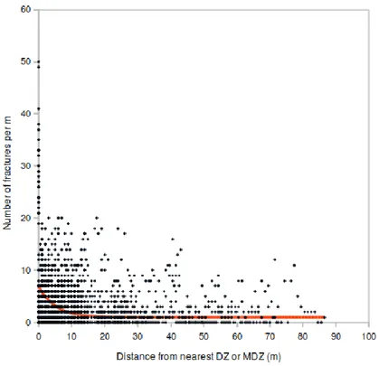
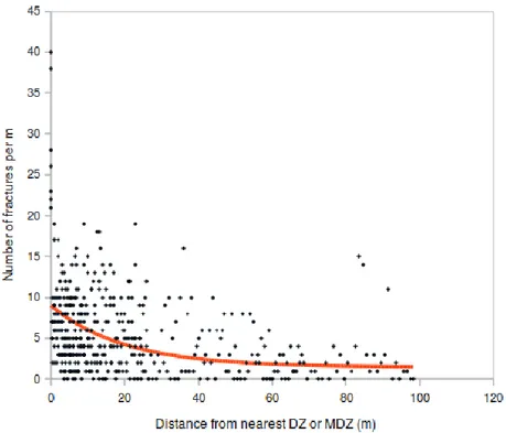
Parameter values estimated by this method are listed in Table 3.1 for FFM01, FFM02, and FFM04 & FFM05 (analysed in combination). Plots comparing the data with the fitted functions are given in in Figures 3.1 through 3.3. The data show a very wide scatter around the fitted functions. The extent to which this scatter can be attributed to stochastic variation and sampling volumes in a discrete network can best be addressed by simulation, as explored in the later sections of this report.
Of the three domains, FFM01 has the lowest background fracture intensity as represented by P∞, but also appears to have the strongest influence of de-formation zones. Since FFM01 is the main host rock for the proposed reposi-tory, this contrast may be of importance for the near-field performance. These estimates can form the basis for an alternative fracture model that is generated sequentially, by simulating larger features (minor deformation zones) first, then smaller features with intensity based on proximity to the nearest MDZ.
The choice of the dividing point between larger and smaller features is es-sentially arbitrary for an analysis based entirely on borehole data, because the sizes of fractures intersecting boreholes are essentially unknown. For the purpose of scoping the potential effects of this type of model, the division is chosen at a fracture diameter of 100 m, which corresponds approximately to the scale of features that are recognized as “minor deformation zones” (MDZs) in SKB's surface-based site investigations.
Table 3.1 Parameter values for deformation-zone influenced fracture-intensity model for Forsmark fracture
domains.
Fracture domain FFM01 FFM02 FFM04 & FFM05
P∞ [m-1] 1 2 1.5
a [–] 6 3.5 5
9
Figure 3.1 Plot of fracture intensity in core-drilled holes as a function of distance from the nearest
defor-mation zone identified by the extended single-hole interpretation, with fitted exponential-halo model in red, for Fracture Domain FFM01.
Figure 3.2 Plot of fracture intensity in core-drilled holes as a function of distance from the nearest
defor-mation zone identified by the extended single-hole interpretation, with fitted exponential-halo model in red, for Fracture Domain FFM02.
10
Figure 3.3 Plot of fracture intensity in core-drilled holes as a function of distance from the nearest
defor-mation zone identified by the extended single-hole interpretation, with fitted exponential-halo model in red, for Fracture Domains FFM04 and FFM05.
Termination relationships
Termination relationships among fracture sets were analysed by Fox et al. (2007, p. 172-173). These results are reproduced here in Tables 3.2 and 3.3 for ease of reference. Termination percentages were only for fracture do-mains FFM02 and FFM03, due to a lack of outcrop data to assess this char-acteristic for other fracture domains. The outcrop mapping methodology did not permit analysis of terminations between the sub-horizontal fracture set and the sub-vertical sets.
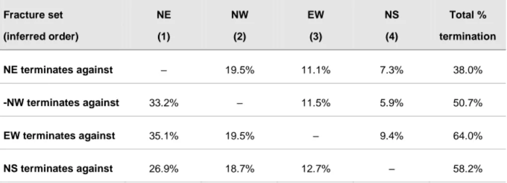
Termination percentages are generally over 50%, with the exception of one fracture set (the NE striking set) in domain FFM02. Thus most fractures identified from outcrops at Forsmark terminate at intersections with other fractures. The highest termination percentage evaluated is 81.9% for the ENE-striking set in FFM03. Despite these findings, termination of fractures at intersections has not been carried forward in the site modelling by SKB. Fox et al. (2007) infer an order of set generation based on the principle that younger fracture sets will more often terminate against older sets, than vice versa. However, from Tables 3.2 and 3.3 it is evident that “older” sets fre-quently terminate against “younger” sets. For example, in FFM02, about
11
20% of the fractures in the NE-striking set terminate against the NW-striking set, despite that the latter is judged to be younger.
A possible alternative interpretation is that many of these fractures were co-eval, and formed as conjugate members of a fault array. From the structural geologic interpretation of the site (Stephens et al., 2007; Stephens et al., 2008), it is further expected that many of the fractures have been reactivated and developed further under different tectonic regimes. In such a system, termination relations will tend to reflect a hierarchy of scales, with subsidi-ary faults terminating at higher-order faults regardless of orientation. Differ-ences in termination percentages among sets can help to indicate which fault orientations most frequently corresponded to the dominant shear plane orien-tations.
This alternative interpretation is supported by visual inspection of the out-crop maps as given in Appendix 8 of Fox et al. (2007), which show many smaller fractures terminating against longer fracture traces. Quantitative analysis of this aspect could be possible, as an extension of this project, by analysis of map data.
Table 3.2 Relative termination percentage between fracture sets and inferred order of fracture set generation
for fracture domain FFM02, adapted from Table 4-80 of Fox et al., 2007.
Fracture set (inferred order) NE (1) NW (2) EW (3) NS (4) Total % termination NE terminates against – 19.5% 11.1% 7.3% 38.0% -NW terminates against 33.2% – 11.5% 5.9% 50.7% EW terminates against 35.1% 19.5% – 9.4% 64.0% NS terminates against 26.9% 18.7% 12.7% – 58.2%
Table 3.3 Relative termination percentage between fracture sets and inferred order of fracture set generation
for fracture domain FFM03, adapted from Table 4-81 of Fox et al., 2007.
Fracture set (inferred order) NW (1) WNW (2) NE (3) NS (4) ENE (5) Total % termina-tion NW terminates against – 16.0% 19.1% 7.2% 10.9% 53.2% WNW terminates against 24.2% – 21.7% 4.5% 9.4% 59.8% NE terminates against 23.1% 15.6% – 5.0% 11.8% 55.5% NS terminates against 25.9% 18.5% 16.7 – 3.7% 64.8%
12
Discussion
Preliminary analysis indicates that the fracture system at Forsmark is spatial-ly organized in the sense that smaller fractures are spatialspatial-ly correlated to larger features (minor deformation zones), and also that smaller fractures tend to terminate against larger structures.
Scaling 3-D fracture intensity measures
The estimates in Table 3.1 can form the basis for an alternative fracture model that is generated sequentially, by simulating larger features (minor deformation zones) first, then smaller features with intensity based on prox-imity to the nearest MDZ.
The function
P
h
above has been derived independent of fracture sets. For application this is treated as a weighting function for the 3-D intensity measures of the individual fracture sets, to yield a model in which fracture intensity varies as a function of the distance to the nearest deformation zone:
P
h
C
P
=
h
P
P 32i 32iHereP32iis the mean 3-D intensity of the ith fracture set in a given fracture domain (as defined in SKB's site descriptive model, used as the base case here), and CP is a normalization factor satisfying:
32i32i
h
=
P
P
V
where the integral is taken over the fracture domain. This is to ensure that the fracture intensity, when averaged over the domain, is equal to that for the base-case. This condition is satisfied when:
h
dV
P
=
C
V P
In principal the normalization factor CP can be estimated by Monte Carlo
integration over the fracture domain for a given realization of MDZs. How-ever, as a practical matter for the implementation method adopted here, de-termining the value of CP is not necessary, since fractures are generated one
at a time until the target value of P32i is reached.
An implicit assumption in this approach is that the intensities of all fracture sets vary in a similar way as a function of h. If this assumption is relaxed so that the intensity of each fracture set varies independently of the others, the result would be a more complex model. For such a model, the analysis would need to be repeated using three-dimensional (P32i) fracture intensity estimates for individual fracture sets, following the analytical correction pro-cedure described by Fox et al. (2007, p. 45-46). This more complex type of model was not attempted in the present study, in favor of testing whether a simpler change in conceptual model could produce significant effects.
13
The estimates given in Table 3.1 are based on one-dimensional (P01) fracture intensity data from along boreholes, which have not been corrected for ori-entation bias. The parameter estimates could also be made more exact by non-linear least-squares fitting (e.g. using the Levenberg-Marquardt algo-rithm rather than manual adjustment). These refinements are desirable but would likely only result in minor changes, compared to the main effect of introducing this spatially heterogeneous model in place of SKB's more ho-mogeneous model.
Two alternative DFN conceptual model variants are suggested to investigate the consequences of this spatial organization for a repository at Forsmark. Both make use of the same fracture set definitions as defined by SKB, in-cluding the fitted probability distributions for fracture orientation, size, and transmissivity. The only differences are as follows:
(1) Spatially correlated variant: Fractures in different size classes are simulated sequentially, starting with the largest class of features. In-tensity for smaller classes of fractures scales with distance from the nearest larger-scale feature (DZ or MDZ), according to the inverse exponential relationship with parameters as defined in Section 3.1. (2) Spatially correlated variant with hierarchical termination: As
for the preceding variant, but with probabilistic termination of smaller fractures at intersections with larger fractures to match (ap-proximately) the observed termination percentages as listed in Ta-bles 3.2 and 3.3.
Priority was given to the first of these variants, which was expected to be more significant than the second.
The second variant (with terminations) is expected to be significant only very close to the repository, where it can affect the discrete connectivity of pathways from deposition holes to larger features. With the method used to calculate equivalent hydraulic conductivity values for assignment to grid features farther from the deposition holes, this level of detail will have no influence.
14
4. Implementation of
alter-native exponential halo
model
Mathematical development and implementation
The exponential halo model was implemented as a new option in the fracgen module of the DFM package, Version 2.3.4.
This required development of a method for stochastic simulation of fracture locations in a non-uniform intensity field of the specified form, rather than as a uniform Poisson process. Three different types of algorithms were consid-ered:
1) Acceptance-rejection method (generating random points by a uni-form Poisson process, then thinning these depending on comparison to a test function based on the exponential-halo model);
2) Spatial binning using an adaptation of the bubble-cover algorithm as described in the DFM user documentation (Geier, 2010h), in which the mean intensity within each bubble is calculated based on Monte Carlo integration of the function P(h) within the bubble volume; and 3) Spatial transformation method in which points simulated by a
uni-form Poisson point process are shifted toward the nearest larger fea-ture.
The first type of algorithm was rejected as it would require generation and testing of close to (a+1) times as many points as are needed, in each case finding the distance to the closest parent feature, and then calculating the test function.
The second approach might well be the fastest (particularly for simulating a large number of fracture centres), but its accuracy would depend on the coarseness of the bubble cover, as well as the convergence of the Monte Car-lo integration.
The spatial transformation approach was therefore chosen for development at this stage of the project, as it produces one fracture per simulated point, and does not depend on the degree of refinement as would be the case for the bubble-cover algorithm.
The steps in the spatial transformation algorithm (derived as part of this pro-ject) are:
1. Generate a point x within a given domain based on a uniform Pois-son process.
2. Calculate the distance H to the nearest point on the closest parent feature F.
15
3. Calculate the expected number of points N(H) that would lie within distance H of F, for a Poisson process of uniform average density. 4. Find the rescaled distance h such that the corresponding expected
number of points n(h) within distance h of F for the exponential halo model P(h|P∞, a,α) is equal to N(H).
5. Shift the point x toward F so that the transformed point x' is at dis-tance h.
Fractures in the child sets are generated by this algorithm one at a time, but each fracture in a child set is independent of each other fracture in the child sets, so in principle this is independent of the sequence. The halo model is created with respect to all of the deformation zones, but the point field inten-sity at a given point x is defined only with respect to the nearest deformation zone (parent feature) F.
The mathematical development of the algorithm makes use of the following geometrical formulae:
Area of 3-D surface within distance η of a disc of radius r
2 2
2η
2π
r
+
πrη
+
=
η
A
Volume within distance η of a disc of radius r
2 2 3 4 2r +πrη+ η πη = η VExpected number of Poisson points within distance H of a disc of radius r
2 2 3 4 2r +πrH+ H πH P = H V P = H N avg avgwhere Pavg is the average intensity of the Poisson process (points per unit
volume).
Expected number of exponential halo points within distance h of a disc of radius r
h αη hdη
η
A
ae
+
P
=
dη
η
A
η
P
=
h
n
0 01
2 αh+
he
αhα
+
πr
α
a
e
b
+
h
+
rh
π
+
h
r
πP
=
h
n
1
4
2h
3
2
2
2
2 3 where: 2 2 4 α + r α π + r α a = b16
Setting n(h) equal to N(H) and dividing both sides by P∞ leads to the
non-linear equation:
H
V
P
P
=
P
h
n
avg The value of Pavg, the average intensity of the Poisson point process which is
required to achieve a given volumetric fracture intensity P32 is generally not known a priori. Pavg is related to P32 by a factor which is a function of the fracture size and orientation distributions for a given fracture domain geome-try. In principle this factor could be estimated by Monte Carlo integration over the domain, for each fracture set.
However, since the method of application will be to generate fractures in each set iteratively until a target value of P32 is reached, and considering that for a sufficiently large domain Pavg approaches P∞ (though is always slightly
larger), here the simplification Pavg/P∞ ≈ 1 is introduced, to yield:
H
V
P
h
n
The function n(h)/P∞ increases monotonically with a continuous derivative
over all values of h > 0, so for a given function value the corresponding val-ue of h is readily obtained by the Newton-Raphson method.
The location of the transformed point is then calculated as:
x
p
H
h
+
p
=
x'
where p is the closest point on the parent feature F, in relation to the Poisson point x.
17
5. Evaluation of alternatives
using borehole data
Analysis
Fracture statistical models
Fracture populations simulated with the alternative (exponential-halo) model were compared with simulations of SKB's GeoDFN model as used by Mu-nier (2010). The GeoDFN model was used for this comparison rather than the HydroDFN model, as non-transmissive fractures contribute to fracture frequency and fracture spacing measures.
Munier (2010) considers three variants of the GeoDFN model for Forsmark, all of which are based on a Poisson process for fracture locations, but which differ in assumptions regarding the fracture size distribution. Here as a base case for reference, we compare with the r0-fixed case, which produces the highest degree of utilization according to the calculations by Munier (2010). Calculations are performed only for fracture domain FFM01, which is the main fracture domain that intersects the planned locations of the repository tunnels; the other fracture domain of concern, FFM06, yields similar utiliza-tion factors according to Munier (2010).
The fracture set definitions used as fracgen input for this base case are listed in Table 5.1. Note that the statistical models for fracture hydraulic properties (transmissivity, storativity, and aperture) are arbitrary and should be disre-garded, as these are not defined for the GeoDFN model (the statistical mod-els used apply to the HydroDFN model, but the GeoDFN contains many ad-ditional fractures that are regarded as non-transmissive, so these are not cor-rectly represented here).
The exponential-halo model uses the same statistics, but treats GeoDFN fractures with r > 100 m as parent features for the smaller fractures. The choice of r = 100 m as the dividing point corresponds approximately to the scale of features that tend to be interpreted as minor deformation zones (MDZs) in SKB's site descriptive model. The method of implementation for the exponential halo model in fracgen is to split each fracture set into two parts depending on fracture radius: r > 100 m (simulated first, for all nine sets defined in the GeoDFN), and r < 100 m (simulated afterwards). Major deformation zones defined by SKB's site investigations also serve as parent features for the child fractures; these are loaded in as deterministic surfaces prior to generating the fractures.
The fracture set definitions used as fracgen input for the alternative (expo-nential-halo) model are listed in Table 5.2. Again, the statistical models for fracture hydraulic properties (transmissivity, storativity, and aperture) are
18
arbitrary and should be disregarded, as these are not defined for the GeoDFN model.
The parameterizations of the parent and child sets are arbitrarily assumed to be equal, apart from the size range limits for each set. Independent parame-terizations of parent and child sets could be considered as a more complex alternative model, but would be difficult to justify with the present data, and would lead to a more complicated comparison with SKB's GeoDFN model.
Sampling along boreholes
The simulated-sampling feature of fracgen was then used to produce and compare synthetic fracture logs for the base-case ( r0-fixed) and alternative (exponential-halo) models. Borehole geometries were taken from data deliv-eries as documented in Chapter 2. Fracture intersections generated from both the base-case (Poisson) model and the exponential halo model were printed to the fracgen log file, then sorted to yield simulated borehole fracture logs. Fracture intersections generated from both the base-case (Poisson) model and the exponential halo model were printed to the fracgen log file, then sorted to yield simulated borehole fracture logs as excerpted in Table 5.3. These results are plotted for an illustrative selection of the deep core-drilled boreholes, in Figures 5.1 through 5.3.
Fracture spacing in actual boreholes
For comparison with the simulations, fracture spacings were also evaluated from Forsmark core logging data. Source data were taken from the SKB-delivered data file p_fract_core_KFM.xls, along with the limits of fracture domain FFM01 in boreholes as shown in Appendix 4 of Olofsson et al. (2007).
The data file was converted to a csv-format file named
p_fract_core_KFM.csv, then processed with an AWK-language script (get_p_fract_core_eshi_FFM01.awk) to extract the data records for fractures inside FFM01. The extracted data were stored as a smaller data file
p_fract_core_eshi_FFM01.csv.
Fracture spacing values were then calculated from the extracted data, simply by sorting the records in this last file by borehole name and borehole posi-tion (using the adjusted posiposi-tion ADJUSTEDSECUP), and calculating the distance between each neighbouring pair of fractures in a given borehole.
19
Table 5.1 Fracture set definitions for implementation of base case model, Forsmark fracture domain FFM01,
deep sub-domain (continued on next page). # Forsmark-SDM Site
# GeoDFN fracture sets for FFM01 (z < -400 m) based on: # SKB TR-10-21 Table A3-1 (Munier, 2010), fixed r0 alternative #
# Arbitrarily:
# (semi-correlated model for transmissivity vs. r) is from Follin 2008. #
Set 1 # NE
Transmissivity Loglinear r 0.5 5.3e-11 1.0 limits -2 2 Storativity Constant 1e-8
Aperture CubicLaw
Radius Powerlaw 3.718 0.039 limits 2.8843 564.2 Location Poisson
Orientation Fisher trend 314.90 plunge 1.30 kappa 20.94 Intensity P32 1.733 unscaled
Set 2 # NS
Transmissivity Loglinear r 0.5 5.3e-11 1.0 limits -2 2 Storativity Constant 1e-8
Aperture CubicLaw
Radius Powerlaw 3.745 0.039 limits 2.8843 564.2 Location Poisson
Orientation Fisher trend 270.10 plunge 5.30 kappa 21.34 Intensity P32 1.292 unscaled
Set 3 # NW
Transmissivity Loglinear r 0.5 5.3e-11 1.0 limits -2 2 Storativity Constant 1e-8
Aperture CubicLaw
Radius Powerlaw 3.607 0.039 limits 2.8843 564.2 Location Poisson
Orientation Fisher trend 230.10 plunge 4.60 kappa 15.70 Intensity P32 0.948 unscaled
Set 4 # SH
Transmissivity Loglinear r 0.5 5.3e-11 1.0 limits -2 2 Storativity Constant 1e-8
Aperture CubicLaw
Radius Powerlaw 3.579 0.039 limits 2.8843 564.2 Location Poisson
Orientation Fisher trend 0.80 plunge 87.30 kappa 17.42 Intensity P32 0.624 unscaled
Set 5 # ENE
Transmissivity Loglinear r 0.5 5.3e-11 1.0 limits -2 2 Storativity Constant 1e-8
Aperture CubicLaw
Radius Powerlaw 3.972 0.039 limits 2.8843 564.2 Location Poisson
Orientation Fisher trend 157.50 plunge 3.10 kappa 34.11 Intensity P32 0.256 unscaled
20
Table 5.1 (ctd) Fracture set definitions for implementation of base case model, Forsmark fracture domain
FFM01, deep sub-domain. Set 6 # EW
Transmissivity Loglinear r 0.5 5.3e-11 1.0 limits -2 2 Storativity Constant 1e-8
Aperture CubicLaw
Radius Powerlaw 3.930 0.039 limits 2.8843 564.2 Location Poisson
Orientation Fisher trend 0.40 plunge 11.90 kappa 13.89 Intensity P32 0.169 unscaled
Set 7 # NNE
Transmissivity Loglinear r 0.5 5.3e-11 1.0 limits -2 2 Storativity Constant 1e-8
Aperture CubicLaw
Radius Powerlaw 4.000 0.039 limits 2.8843 564.2 Location Poisson
Orientation Fisher trend 293.80 plunge 0.00 kappa 21.79 Intensity P32 0.658 unscaled
Set 8 # SH2
Transmissivity Loglinear r 0.5 5.3e-11 1.0 limits -2 2 Storativity Constant 1e-8
Aperture CubicLaw
Radius Powerlaw 3.610 0.039 limits 2.8843 564.2 Location Poisson
Orientation Fisher trend 164.00 plunge 52.60 kappa 35.43 Intensity P32 0.081 unscaled
Set 9 # SH3
Transmissivity Loglinear r 0.5 5.3e-11 1.0 limits -2 2 Storativity Constant 1e-8
Aperture CubicLaw
Radius Powerlaw 3.610 0.039 limits 2.8843 564.2 Location Poisson
Orientation Fisher trend 337.90 plunge 52.90 kappa 17.08 Intensity P32 0.067 unscaled
21
Table 5.2 Fracture set definitions for implementation of halo model, Forsmark fracture domain FFM01, deep
sub-domain (continued on following pages). # Forsmark-SDM Site
# GeoDFN fracture sets for FFM01 (z < -400 m) based on: # SKB TR-10-21 Table 5-1 (Munier, 2010)
# # Arbitrarily:
# (semi-correlated model for transmissivity vs. r) is from Follin 2008. #
Set 1 # NE
Transmissivity Loglinear r 0.5 5.3e-11 1.0 limits -2 2 Storativity Constant 1e-8
Aperture CubicLaw
Radius Powerlaw 3.718 0.039 limits 100 564.2 Location Poisson
Orientation Fisher trend 314.90 plunge 1.30 kappa 20.94 Intensity P32 1.733 unscaled
Set 2 # NS
Transmissivity Loglinear r 0.5 5.3e-11 1.0 limits -2 2 Storativity Constant 1e-8
Aperture CubicLaw
Radius Powerlaw 3.745 0.039 limits 100 564.2 Location Poisson
Orientation Fisher trend 270.10 plunge 5.30 kappa 21.34 Intensity P32 1.292 unscaled
Set 3 # NW
Transmissivity Loglinear r 0.5 5.3e-11 1.0 limits -2 2 Storativity Constant 1e-8
Aperture CubicLaw
Radius Powerlaw 3.607 0.039 limits 100 564.2 Location Poisson
Orientation Fisher trend 230.10 plunge 4.60 kappa 15.70 Intensity P32 0.948 unscaled
Set 4 # SH
Transmissivity Loglinear r 0.5 5.3e-11 1.0 limits -2 2 Storativity Constant 1e-8
Aperture CubicLaw
Radius Powerlaw 3.579 0.039 limits 100 564.2 Location Poisson
Orientation Fisher trend 0.80 plunge 87.30 kappa 17.42 Intensity P32 0.624 unscaled
Set 5 # ENE
Transmissivity Loglinear r 0.5 5.3e-11 1.0 limits -2 2 Storativity Constant 1e-8
Aperture CubicLaw
Radius Powerlaw 3.972 0.039 limits 100 564.2 Location Poisson
Orientation Fisher trend 157.50 plunge 3.10 kappa 34.11 Intensity P32 0.256 unscaled
22
Table 5.2 (ctd) Fracture set definitions for implementation of halo model, Forsmark fracture domain FFM01,
deep sub-domain.
Set 6 # EW
Transmissivity Loglinear r 0.5 5.3e-11 1.0 limits -2 2 Storativity Constant 1e-8
Aperture CubicLaw
Radius Powerlaw 3.930 0.039 limits 100 564.2 Location Poisson
Orientation Fisher trend 0.40 plunge 11.90 kappa 13.89 Intensity P32 0.169 unscaled
Set 7 # NNE
Transmissivity Loglinear r 0.5 5.3e-11 1.0 limits -2 2 Storativity Constant 1e-8
Aperture CubicLaw
Radius Powerlaw 4.000 0.039 limits 100 564.2 Location Poisson
Orientation Fisher trend 293.80 plunge 0.00 kappa 21.79 Intensity P32 0.658 unscaled
Set 8 # SH2
Transmissivity Loglinear r 0.5 5.3e-11 1.0 limits -2 2 Storativity Constant 1e-8
Aperture CubicLaw
Radius Powerlaw 3.610 0.039 limits 100 564.2 Location Poisson
Orientation Fisher trend 164.00 plunge 52.60 kappa 35.43 Intensity P32 0.081 unscaled
Set 9 # SH3
Transmissivity Loglinear r 0.5 5.3e-11 1.0 limits -2 2 Storativity Constant 1e-8
Aperture CubicLaw
Radius Powerlaw 3.610 0.039 limits 100 564.2 Location Poisson
Orientation Fisher trend 337.90 plunge 52.90 kappa 17.08 Intensity P32 0.067 unscaled
Set 10 # NE child
Transmissivity Loglinear r 0.5 5.3e-11 1.0 limits -2 2 Storativity Constant 1e-8
Aperture CubicLaw
Radius Powerlaw 3.718 0.039 limits 2.8843 100
Location Halo P 1 a 6 alpha 0.2 parents 0 1 2 3 4 5 6 7 8 9 Orientation Fisher trend 314.90 plunge 1.30 kappa 20.94 Intensity P32 1.733 unscaled
Set 11 # NS child
Transmissivity Loglinear r 0.5 5.3e-11 1.0 limits -2 2 Storativity Constant 1e-8
Aperture CubicLaw
Radius Powerlaw 3.745 0.039 limits 2.8843 100
Location Halo P 1 a 6 alpha 0.2 parents 0 1 2 3 4 5 6 7 8 9 Orientation Fisher trend 270.10 plunge 5.30 kappa 21.34 Intensity P32 1.292 unscaled
23
Table 5.2 (ctd) Fracture set definitions for implementation of halo model, Forsmark fracture domain FFM01,
deep sub domain.
Set 12 # NW child
Transmissivity Loglinear r 0.5 5.3e-11 1.0 limits -2 2 Storativity Constant 1e-8
Aperture CubicLaw
Radius Powerlaw 3.607 0.039 limits 2.8843 100
Location Halo P 1 a 6 alpha 0.2 parents 0 1 2 3 4 5 6 7 8 9 Orientation Fisher trend 230.10 plunge 4.60 kappa 15.70 Intensity P32 0.948 unscaled
Set 13 # SH child
Transmissivity Loglinear r 0.5 5.3e-11 1.0 limits -2 2 Storativity Constant 1e-8
Aperture CubicLaw
Radius Powerlaw 3.579 0.039 limits 2.8843 100
Location Halo P 1 a 6 alpha 0.2 parents 0 1 2 3 4 5 6 7 8 9 Orientation Fisher trend 0.80 plunge 87.30 kappa 17.42 Intensity P32 0.624 unscaled
Set 14 # ENE child
Transmissivity Loglinear r 0.5 5.3e-11 1.0 limits -2 2 Storativity Constant 1e-8
Aperture CubicLaw
Radius Powerlaw 3.972 0.039 limits 2.8843 100
Location Halo P 1 a 6 alpha 0.2 parents 0 1 2 3 4 5 6 7 8 9 Orientation Fisher trend 157.50 plunge 3.10 kappa 34.11 Intensity P32 0.256 unscaled
Set 15 # EW child
Transmissivity Loglinear r 0.5 5.3e-11 1.0 limits -2 2 Storativity Constant 1e-8
Aperture CubicLaw
Radius Powerlaw 3.930 0.039 limits 2.8843 100
Location Halo P 1 a 6 alpha 0.2 parents 0 1 2 3 4 5 6 7 8 9 Orientation Fisher trend 0.40 plunge 11.90 kappa 13.89 Intensity P32 0.169 unscaled
Set 16 # NNE child
Transmissivity Loglinear r 0.5 5.3e-11 1.0 limits -2 2 Storativity Constant 1e-8
Aperture CubicLaw
Radius Powerlaw 4.000 0.039 limits 2.8843 100
Location Halo P 1 a 6 alpha 0.2 parents 0 1 2 3 4 5 6 7 8 9 Orientation Fisher trend 293.80 plunge 0.00 kappa 21.79 Intensity P32 0.658 unscaled
Set 17 # SH2 child
Transmissivity Loglinear r 0.5 5.3e-11 1.0 limits -2 2 Storativity Constant 1e-8
Aperture CubicLaw
Radius Powerlaw 3.610 0.039 limits 2.8843 100
Location Halo P 1 a 6 alpha 0.2 parents 0 1 2 3 4 5 6 7 8 9 Orientation Fisher trend 164.00 plunge 52.60 kappa 35.43 Intensity P32 0.081 unscaled
24
Table 5.2 (ctd) Fracture set definitions for implementation of halo model, Forsmark fracture domain FFM01,
deep sub-domain.
Set 18 # SH3 child
Transmissivity Loglinear r 0.5 5.3e-11 1.0 limits -2 2 Storativity Constant 1e-8
Aperture CubicLaw
Radius Powerlaw 3.610 0.039 limits 2.8843 100
Location Halo P 1 a 6 alpha 0.2 parents 0 1 2 3 4 5 6 7 8 9 Orientation Fisher trend 337.90 plunge 52.90 kappa 17.08 Intensity P32 0.067 unscaled
Table 5.3. Excerpt of a simulated fracture log for multiple boreholes. L is distance along the borehole to the
given fracture intersection, strike & dip of the fracture are given in degrees following the usual right-hand convention for dip, T is fracture transmissivity, (X,Y,Z) are the global coordinates of the fracture's intersection with the centre line of a given borehole segment, and (nx, ny, nz) are the components of the fracture normal vector.
Borehole L (m) Strike Dip T(m2/s) X (m) Y (m) Z (m) nx ny nz
HFM01 140.31 358.9 8.2 3.76e-06 1631499.98 6699621.85 -136.64 -0.003 0.142 0.990 HFM01 147.99 19.0 1.2 3.63e-08 1631501.07 6699622.59 -144.21 0.007 0.019 1.000 HFM01 168.92 180.2 10.6 2.99e-05 1631504.23 6699624.80 -164.77 -0.001 -0.183 0.983 HFM01 172.31 213.1 8.8 1.16e-05 1631504.77 6699625.19 -168.10 -0.083 -0.128 0.988 HFM01 187.54 72.8 27.3 9.03e-06 1631507.31 6699627.04 -182.99 0.439 0.136 0.888 HFM01 192.48 247.8 10.0 6.07e-07 1631508.17 6699627.67 -187.82 -0.160 -0.065 0.985 HFM01 194.06 270.0 36.5 9.44e-07 1631508.44 6699627.88 -189.36 -0.595 0.001 0.804 HFM01 194.41 281.0 46.9 8.07e-06 1631508.51 6699627.92 -189.71 -0.717 0.139 0.683 HFM16 118.94 148.5 21.6 4.17e-08 1632468.43 6699717.95 -115.25 0.193 -0.314 0.930 HFM16 122.74 20.2 17.8 9.34e-06 1632469.00 6699717.52 -118.99 0.106 0.287 0.952 HFM16 128.23 140.5 15.1 7.37e-08 1632469.90 6699716.85 -124.36 0.165 -0.201 0.966 HFM16 129.08 63.6 30.4 8.80e-05 1632470.04 6699716.75 -125.19 0.454 0.225 0.862 HFM17 108.95 338.2 35.8 5.28e-08 1633263.24 6699471.67 -104.53 -0.217 0.543 0.811 HFM20 100.75 355.5 20.6 1.53e-05 1630776.53 6700193.17 -97.59 -0.028 0.350 0.936 HFM20 111.34 36.4 49.0 2.10e-06 1630776.43 6700193.38 -108.18 0.448 0.607 0.656 HFM20 114.94 190.2 25.9 1.77e-04 1630776.37 6700193.43 -111.78 -0.077 -0.430 0.899 HFM20 118.39 161.9 32.6 7.29e-05 1630776.31 6700193.46 -115.23 0.168 -0.513 0.842 HFM20 128.50 37.8 5.1 6.24e-06 1630776.09 6700193.45 -125.34 0.055 0.070 0.996 HFM20 135.59 57.0 11.4 1.55e-06 1630775.90 6700193.41 -132.42 0.166 0.108 0.980 HFM20 136.13 134.1 46.1 7.88e-07 1630775.89 6700193.40 -132.96 0.517 -0.501 0.694 HFM20 140.03 95.1 23.8 2.57e-07 1630775.77 6700193.37 -136.86 0.403 -0.036 0.915 HFM20 142.28 331.0 54.0 1.86e-07 1630775.70 6700193.34 -139.11 -0.392 0.708 0.588 ...
25
Results
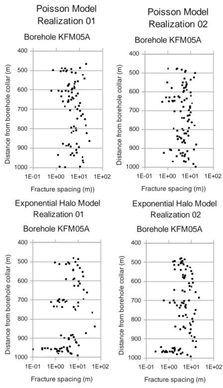
The results are plotted for an illustrative selection of the deep core-drilled boreholes, in Figures 5.1 through 5.3. Results are plotted as fracture spacing versus depth (rather than as interval transmissivity vs. depth as in the preced-ing memorandum, Geier 2010d, since the statistical model for fracture transmissivity is arbitrary as discussed above).
A noticeable difference between the two models, when plotted in this way, is that fracture spacing values appear to be spatially correlated with respect to distance along the boreholes. The exponential-halo model tends to produce long intervals with very few fractures (most strikingly, the interval from 760 m to 880 m depth in KFM05A, in realization 1).
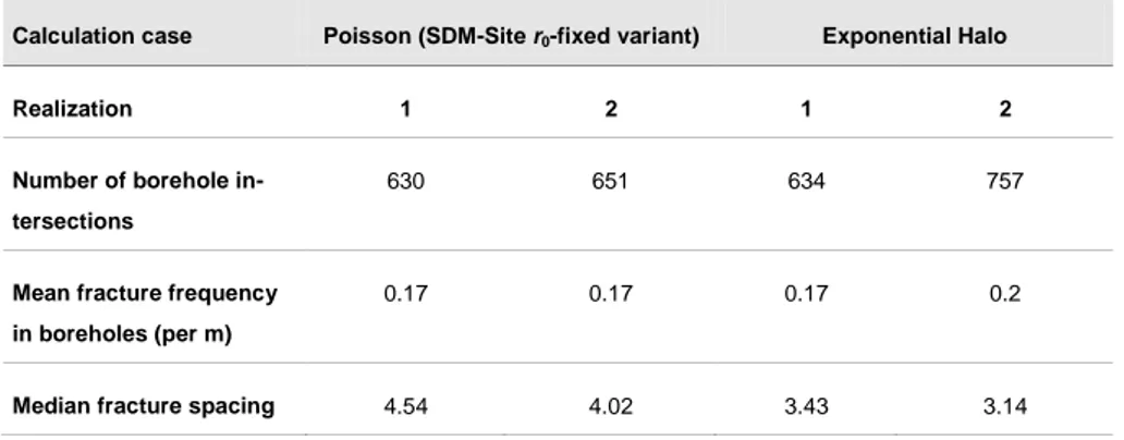
As seen from Table 5.4, the total number of fractures that intersect the bore-holes in fracture domain FFM01, is similar for two realizations of the base-case model, and one realization of the exponential-halo model. The other realization of the exponential-halo model yields about 20% more intersec-tions with boreholes. Similar results are obtained for mean fracture frequen-cy. This is apparently due to chance location of a few stochastic “parent” fractures in the second realization of the exponential-halo model, which leads to more clusters of “child” fractures that intersect the boreholes. The median fracture spacings for these two realizations of the exponential-halo model are lower by 15% to 22% than for the realization of the base-case model that produced the lowest median fracture spacing. However due to the substantial variability in this measure between realizations (+/- 6% for the base-case and +/- 5% for the halo model), additional realizations may be needed to determine if median fracture spacing is a robust statistic for com-parison between models.
Table 5.4 Statistical summary of results from simulations of borehole sampling comparing two different
mod-els of the fracture population in Fracture Domain FFM01 at Forsmark. Results are combined for all 17 bore-holes that penetrated FFM01 (at the time of the data freeze for the data delivery used as the basis for these calculations), for two different realizations of each model.
Calculation case Poisson (SDM-Site r0-fixed variant) Exponential Halo
Realization 1 2 1 2
Number of borehole in-tersections
630 651 634 757
Mean fracture frequency in boreholes (per m)
0.17 0.17 0.17 0.2
26
Figure 5.1 Simulated fracture logs for Fracture Domain FFM01, Borehole KFM01A.
1E-01 1E+00 1E+01 1E+02 400 500 600 700 800 900 1000
Poisson Model
Realization 01
Borehole KFM01A Fracture spacing (m)) D ist a n ce f ro m b o re h o le co ll a r (m)1E-01 1E+00 1E+01 1E+02 400 500 600 700 800 900 1000
Poisson Model
Realization 02
Borehole KFM01A Fracture spacing (m)) D ist a nce f ro m b o re h o le co ll a r (m )1E-01 1E+00 1E+01 1E+02 400 500 600 700 800 900 1000
Exponential Halo Model Realization 01 Borehole KFM01A Fracture spacing (m) D ist a n ce f ro m b o re h o le co ll a r (m)
1E-01 1E+00 1E+01 1E+02 400 500 600 700 800 900 1000
Exponential Halo Model Realization 02 Borehole KFM01A Fracture spacing (m) D ist a n ce f ro m b o re h o le co ll a r (m)
27
Figure 5.2 Simulated fracture logs for Fracture Domain FFM01, Borehole KFM05A.
1E-01 1E+00 1E+01 1E+02 400 500 600 700 800 900 1000
Poisson Model
Realization 01
Borehole KFM05A Fracture spacing (m)) D ist a n ce f ro m b o re h o le co ll a r (m)1E-01 1E+00 1E+01 1E+02 400 500 600 700 800 900 1000
Poisson Model
Realization 02
Borehole KFM05A Fracture spacing (m)) D ist a n ce f ro m b o re h o le co ll a r (m)1E-01 1E+00 1E+01 1E+02 400 500 600 700 800 900 1000
Exponential Halo Model Realization 01 Borehole KFM05A Fracture spacing (m) D ist a n ce f ro m b o re h o le co ll a r (m )
1E-01 1E+00 1E+01 1E+02 400 500 600 700 800 900 1000
Exponential Halo Model Realization 02 Borehole KFM05A Fracture spacing (m) D ist a n ce f ro m b o re h o le co ll a r (m)
28
Figure 5.3 Simulated fracture logs for Fracture Domain FFM01, Borehole KFM07A.
1E-01 1E+00 1E+01 1E+02 400 500 600 700 800 900 1000
Poisson Model
Realization 02
Borehole KFM07A Fracture spacing (m)) D ist a n ce f ro m b o re h o le co ll a r (m)1E-01 1E+00 1E+01 1E+02 400 500 600 700 800 900 1000
Poisson Model
Realization 01
Borehole KFM07A Fracture spacing (m)) D ist a n ce f ro m b o re h o le co ll a r (m)1E-01 1E+00 1E+01 1E+02 400 500 600 700 800 900 1000
Exponential Halo Model Realization 01 Borehole KFM07A Fracture spacing (m) D ist a n ce f ro m b o re h o le co ll a r (m)
1E-01 1E+00 1E+01 1E+02 400 500 600 700 800 900 1000
Exponential Halo Model Realization 02 Borehole KFM07A Fracture spacing (m) D ist a n ce f ro m b o re h o le co ll a r (m )
29
The cumulative density functions for fracture spacing (Figure 5.4) also show substantial distinctions between the two models, as well as between two real-izations of a given model. A Kolmogorov-Smirnov test comparing the halo model to the Poisson model (comparing the closest realizations of each) yields a probability of only 0.08% that the spacing samples are drawn from the same parent distribution; in other words this hypothesis can be rejected at a significance level of 99.9%.
The corresponding probability for the observed difference between realiza-tions of the Poisson model is 40%. The probability for the observed differ-ences between realizations of the halo model is 35%. Thus the differdiffer-ences between realizations of a given model are much less significant than the dif-ference between models. This result suggests that comparison of fracture spacing distributions could be a way to distinguish between these two mod-els based on borehole data.
However, fracture spacing distributions calculated from actual borehole data from Fracture Domain FFM0, as also shown in Figure 5.4, show large dif-ferences with both the Poisson model and the exponential halo model. This is true regardless of whether fracture spacings are calculated based on (1) all fractures, (2) only fractures that were characterized either as open or partly open/partly sealed, or (3) only open fractures. Possible explanations for this large discrepancy are discussed in the following section.
30
Figure 5.4 Comparison of two realizations of the base case (Poisson process) vs. two realizations of the
exponential-halo model in terms of the cumulative and incremental frequency of simulated fracture spacing, for Forsmark fracture domain FFM01. Each data point on the incremental plot represents the fraction of the points that are within a bin covering 1/4 order of magnitude on the logarithmic scale. Also shown for compari-son on the first plot are the measured cumulative distributions of fracture spacing in borehole sections that are within FFM01, for three different classifications of these fractures: open fractures only, open fractures plus partly sealed fractures, and all fractures (including sealed fractures).
31
Discussion
Simulations of borehole sampling in Fracture Domain FFM01 show that the base-case (Poisson) model should be distinguishable from the exponential halo model, for this idealized type of sampling. The main differences are that exponential halo model shows longer intervals of borehole with no conduc-tive fractures, as well as intervals of closely spaced fractures, which at least qualitatively corresponds to a recognized characteristic of the Forsmark site. The possibility that clustering of fractures in the halo model is significant for large-scale connectivity and groundwater flow is explored by site-scale modelling in Chapter 8.
However, simulated borehole sampling for both models shows large discrep-ancies with actual fracture spacing data from core-drilled holes in FFM01. This is true even when only fractures mapped as “open” are considered. The simulated spacing distribution for the exponential halo model is marginally closer to the curves for the actual data than the simulated spacing distribu-tion for the Poisson model, but the discrepancies are so large for both models that that not much meaning can be attached to this observation.
One explanation for these large discrepancies is the practical necessity to use a finite, minimum fracture size in the simulated sampling. The simulations include only fractures with radii of 0.5 m or larger. According to the fitted power-law model for fracture size, there should be vast numbers of smaller fractures that are still larger than the borehole radius (on the order of 10 cm). This is only partly compensated for by the fact that smaller fractures have lower probabilities of intersecting a borehole.
This appears to be a practical difficulty in comparing borehole data with simulations of borehole sampling. Unless the simulations are extended to include very small fractures down to the scale of 10 cm – which requires much longer computation times -- comparison between actual and simulated datasets in terms of fracture spacing might not be meaningful. Spacing data are also sensitive to the classification of fractures during borehole mapping (i.e. as sealed vs. open), and to the treatment of intensively fractured zones. Mapping of fractures in underground tunnels (considered in the next section of this report) may be a more favourable situation for comparing models to data, since there is the possibility to limit the size range of fractures that en-ter into spacing calculations.
Based on comparison of borehole sampling simulations to actual borehole data there appears to be no reason to favour the Poisson model over the ex-ponential halo model; if anything, the exex-ponential halo model is marginally better. Thus it appears useful to propagate this model further to analyse its consequences for repository performance.
32
6. Potential to distinguish
al-ternatives in repository
tunnels
This chapter addresses the research question:
To what extent can data obtained in the repository construction phase reasonably be expected to limit uncertainties with regard to DFN size distributions and spatial/structural relationships among fractures, for the rock at repository depth?
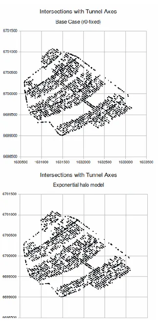
This question is addressed by means of simulated sampling along tunnels based on SKB's most recently proposed repository layout. Comparisons are made with respect to alternative DFN models proposed by SKB (SKB 2008; Munier, 2010), and an additional alternative model (exponential halo model) that is based on the same borehole data analysed by SKB, but which produc-es stronger clustering of small fracturproduc-es around major and minor deformation zones.
The method of investigation is based on simulated sampling along tunnels (based on SKB's most recently proposed repository layout) to evaluate the likelihood of being able to discriminate among viable alternative DFN mod-els during the construction phase.
The first stage of analysis tests the potential for underground observations to discriminate between alternative models for the spatial organization of frac-tures. This is done by sampling fracture intersections along the tunnel axes, and comparing between models in terms of the spacing distribution. From previous work (Geier, 2010d and preceding chapters of this report) this was expected to be an effective way for discriminating between SKB's model based on a Poisson process for fracture location, and a proposed alternative based on the exponential halo model.
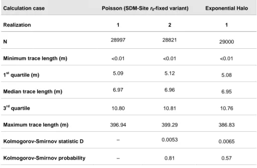
The second stage of analysis tests the potential for fracture sampling along tunnel walls to distinguish between alternative assumptions regarding the DFN size distribution. In this case, the comparison is among alternative models that were developed by SKB (SKB 2008; Munier, 2010). The basic procedure was to generate stochastic realizations of the fracture population, calculate the intersections with tunnel walls, and compare the models in terms of the resulting distribution of trace lengths.