Forming an Inventory Control Policy and Forecasting Model for an E-Commerce Company

(1)

FORMING AN INVENTORY CONTROL POLICY AND

FORECASTING MODEL FOR AN E-COMMERCE

COMPANY

- A study at LSBolagen

Department of Industrial Management and Logistics Lund University, Faculty of Engineering, LTH 2019

Authors: Patrik Lorentsson Nilan Nabavieh

(2)

(3)

iii

Acknowledgements

This thesis concludes the authors’ education of M.Sc. within Industrial Engineering & Management at Faculty of Engineering at Lund University. The thesis consists of many work hours and dedication. However, the thesis would not been brought to completion if it was not for the support of the authors’ supervisors. Thus, the authors would like to give their sincere gratitude to Erik Sondén and Per Lindström for their essential cooperation and Johan Marklund for his guidance and support throughout the project. Another great thanks to the people involved at the case company for their vital help and information for developing the thesis.

Lund, May 2019

(4)

(5)

v

Abstract

Title: Developing an Inventory Control Policy and Forecasting Model for an

E-Commerce Company

Authors: Patrik Lorentsson & Nilan Nabavieh

Supervisor: Johan Marklund, Department of Industrial Management and Logistics

Background: Increasingly competitive business environments forces companies to

develop better control of the material flows in their supply chain. Inventories are often kept in large amounts in order to buffer against uncertainties, resulting in high average holding costs. An important part in controlling this flow of material and inventory is to decide upon when to order and how much. Two important components when evaluating these two, is the inventory policy used as well as the method of forecasting.

Purpose: Forming a basic inventory policy and forecasting model for the warehouse in

Sweden.

Research Questions: (1) How can the inventory policy for the warehouse in Sweden be

improved? (2) What is an adequate forecasting model for the purchasing department?

Methodology: In this thesis, frameworks presented by Yin (2009) and Hillier &

Liebermann (2010) are used to construct the research approach. An initial analysis of the problem presented was conducted in order to properly identify the intended problem. Following this, an analytical analysis of gathered data was conducted to analyse the current performance of the company. Finally, models based on well-known theory were

constructed to represent the new inventory policy and forecasting method.

Conclusion: A simple inventory policy could be constructed. Lack of historical data and

previous analysis meant that an exact representation of the current situation could not be constructed. The demand could be approximated to follow a normal distribution. As the company currently orders in batches, a continuous review (R, Q) policy was chosen. It was found that the inventory levels could be decreased in almost all cases when setting 95 % fill rate constraint. Due to lack of historical data, an adequate forecasting model could not be decided upon. Instead Alternative Forecasting Application Models (AFAMs)

(6)

vi

representing the different models were developed for choosing a suitable forecasting model in the future.

(7)

vii

Table of abbreviations

A - Ordering cost (fixed)

AFAM – Alternative Forecasting Application Model EOQ - Economic Order Quantity

ERP - Enterprise Resource Planning h - Holding cost rate (SEK/year) IL - Inventory Level

IP - Inventory Position KS - Kolmogorov-Smirnov L - Lead time

MAD - Mean Absolute Deviation MOQ - Minimum Order Quantity MTS - Make-To-Stock

OR - Operations Research Q - Batch Quantity Size R -Reorder Point

SCM - Supply Chain Management SKU - Stock Keeping Unit T – Review Period

WMS – Warehouse Management System 3PL – Third-party Logistics

(8)

(9)

ix

1. Introduction

This section will describe the background of the master thesis as well as an introduction to the case company. The identified problem is discussed with the identified research questions and delimitation.

1.1 Background

In today’s business world, companies are facing very demanding customers that will take their business elsewhere if they are not satisfied. Requirements such as short lead times and the ability to be flexible with customisation of products puts a big pressure on competing organisations (Christopher, 2011). As a result, Supply Chain Management (SCM), i.e. the control of material flows from suppliers of raw material to customers, is a crucial problem for organisations and its strategic importance has been recognised by top management. Total investment in inventories is enormous, and as such, there is large improvement potential regarding the amount of tied-up capital in warehouses (Axsäter, 2006).

However, sometimes large quantity of stocks is a necessity. The two main reasons for having large stocks are the economies of scale of ordering products in batches and the uncertainties within a supply chain. Demand can be difficult to forecast and could stem from different order patterns by customer resulting in high variability, proving that demand management is a key aspect to improve a company’s SCM (Lambert, & Cooper, 2000). Supply is often dependent on actors upstream in the SC. These factors in

combination with lead times in both production and distribution creates a need to apply safety stocks to operations. To mitigate the impacts of these factors, adopting appropriate inventory policies can reduce their inventory. (Axsäter, 2006)

1.2 Company description

LSBolagen is an e-commerce company with web sites in the Nordics, UK, Germany and France. Their office is located in Ängelholm, Sweden, with approximately 30 employees as of 2018. They are specialised in durable goods and retail products such as wine cabinets, large range cookers and table tennis products. The main goal of LSBolagen is to deliver their range of products to all of Europe with short lead times and low cost.

(14)

2

LSBolagen is a growing company with a turnover of 100 MSEK in 2017. Their present business model involves purchasing from both Europe and China. One warehouse is located in Klippan, Sweden, and the other in the UK. The warehouse in the UK is rented through a 3PL, from where they have daily deliveries to the eight countries they are operating in.

(15)

3

1.3 Problem formulation

All products of LSBolagen are Made To Stock (MTS), resulting in high amount of tied up capital due to expensive SKUs. At present, purchasing of products at LSBolagen is done irregularly based on the company’s own decision model. This decision model is based on a mean-average assessment, considering the sales data of previous months to produce a forecast. Procurement is then decided upon with a formula taking into consideration the following data on a three-monthly basis: stock-on hand, amount in transit to customer, historical sales and the expected quantity to be delivered from suppliers. The resulting value for each SKU is then individually assessed and compared to the general reorder points used. Long lead times and quantity limitations from suppliers further complicates the process as products often must be consolidated to fill up containers to a certain amount.

Recently, the company has found a need to assess and evaluate their inventory

management process. There has been no previous analysis of whether the used reorder points are adequate for their processes or if they should be changed. As such, there is a need to develop an evaluation framework for the performance of SKUs in stock. Which SKUs have been over- and under-procured and in what periods, what implications does backorders have for sales and what could the optimal reordering points for the purchasing department be. Furthermore, as purchasing decision is done based on historical data, there is a need to develop a forecasting tool for decision making.

Additionally, as LSBolagen is an international company with a satellite warehouse in the UK, there is a need to further coordinate assortments between the main warehouse in Sweden and the satellite warehouse in the UK.

(16)

4

1.4 Purpose of the study and research questions

The purpose of the master thesis is first to analyse the current purchasing process and inventory policy used by the company, then to propose and evaluate an improved inventory and forecasting policy adequate for the company’s operations. The thesis will answer the following research questions:

1. How can the inventory policy for the warehouse in Sweden be improved? 2. What is an adequate forecasting model for the purchasing department?

1.5 Delimitations

The study will be conducted for the case company’s main warehouse in Klippan. As LSBolagen has around 400 SKUs, only key articles in the wine cabinet category presented by the case company will be analysed. Furthermore, as this is the first attempt to fit a theoretical inventory policy to their practice, the model will be kept simple. The focus will be to minimise the average stock levels following a service level constraint. We will not change the method of current operations, e.g. choice of suppliers. The final

implementation of a new inventory policy will be done by the company. Further delimitations will be discussed in later sections.

(17)

5

2. Methodology

This section will present, describe and motivate the chosen research strategy for this study. The purpose is to explain how the study has been performed and how valid and reliable the obtained results are.

2.1 Research approach

As this study is based on practical inventory control problems identified by the company, a standardised method for operations research (OR) projects has been chosen for this thesis. The OR approach can be divided into the following 6 phases:

1. Define the problem and gather the relevant data 2. Formulate a mathematical model to represent the study

3. Develop a computer-based procedure for deriving solutions to the problem from the model

4. Test the model and refine it as needed 5. Preparing to apply the model

6. Implementation (Hillier, & Lieberman, 2010)

2.1.1 Define the problem and gather relevant data

The nature of practical problems encountered by OR teams is often vague and not precisely defined. Therefore, the initial phase of any OR project is to develop a well-defined definition of the objective to be solved and what constraints can be identified. Before moving forward, it is important to maintain a holistic approach for the given objective as an OR study should aim to optimize the whole system and not just one function. As such, the definition of the objective should be conducted in collaboration with management. After the definition has been properly defined, necessary data has to be gathered from the company. As data from both inventory systems and ERPs can be quite extensive, necessary time has to be allocated to the data mining process including cleaning the data and identifying relevant data and interesting patterns. (Ibid.)

2.1.2 Formulate a mathematical model to represent the study

After the objective is properly defined, the next step is to re-formulate this problem to be convenient for analysis. The conventional OR-approach is to construct a mathematical model which represents the essence of the problem. A first step when constructing a

(18)

6

model is to begin with a very basic model and then move towards more elaborate models - until a model which sufficiently covers the complexity of the problem is found. (Ibid.)

2.1.3 Develop a computer-based procedure

With a mathematical model created, the next step is to analyse the outcome of the model. If a model is created to find an optimal solution, it has to be recognized that it is only optimal for the model at hand and the assumptions that define it. As the model is an idealized rather than exact representation of the actual problem, there are no guarantees that the best possible solution to the real system has been found. However, a well formulated and valid model should be a good approximation of the real problem.

Furthermore, research suggests that rather than focusing on optimization of the problem. Instead focus should be on satisficing, reaching results which enables multiple goals to be met. In order to mitigate the risk of the result being an optimal solution with low practical value, a thorough post-optimality analysis needs to be conducted. This can be seen as a what-if analysis to see what impacts other scenarios would have on the optimal solutions. By conducting this sensitivity-analysis, it is possible to identify which parameters are sensitive, i.e. they can’t be changed without changing the optimal solution. (Ibid.)

2.1.4 Test the model and refine it as needed

A first draft of a mathematical model often contains some flaws. It could be that it does not incorporate the right parameters or constraints, as it is hard to gain thorough

understanding of all the aspects of the problem. However, as a mathematical model is an abstract construction of reality, it requires some extent of assumptions for the model to be tractable. Therefore, an important part of the analysis is to ensure that the model is a valid representation of the problem. A proper criterion when ensuring the validity of a model, is to evaluate the model outcome for alternative courses of action. The obtained results should follow what would happen in the real world. (Ibid.)

However, it is difficult to create a model that is valid for all cases. Because they are often problem specific. A systematic approach to validate a model is to use a retrospective test. This test involves reconstructing the past using historical data and then check how the model and the resulting solution would have performed in this scenario. A disadvantage of this test is that it uses the same data which were used to guide the construction of the model in the initial stage. However, if the past can be deemed as a satisfactory

(19)

7

2.1.5 Preparing to apply the model

After the model has been developed and tested it is time to prepare for implementation. If the aim of the model is to be used repeatedly, the next step is to ensure that the user understands the model and how it should be used. The system describing the application should include, model, solution procedure and operating procedures for implementation. (Ibid.)

2.1.6 Implementation

The final step of the OR-study includes the final implementation of the results of the model. This should be carried out in a number of steps. First, the OR-team gives

management an explanation of the new system and how it relates to operating procedures. Next, the two parties share responsibility when launching the new system. Throughout the new user period, it is important for the OR-team to obtain feedback on the performance of the system. This in order to be able to change it if the assumptions are found to no longer be valid. A final step is the documentation of the methodology used in the study in order for it to be reproducible in the future. (Ibid.)

To support this OR-study, a literature review and mapping of the current processes will be conducted in parallel to the study.

2.2 Research quality

According to Yin (2009), research design represents a set of logical statements. However, it is also possible to judge the quality of the design according to certain logical tests. Generally, four tests are used for establishing empirical research. These four tests are:

● Construct validity ● Internal validity ● External validity ● Reliability

2.2.1 Construct validity

The first step in testing the quality is to identify the correct measures for the study. In order to do this, there are three different tactics. The first tactic is using multiple sources of evidence for investigation, for encouraging convergent lines of inquiry. This tactic is

(20)

8

relevant during the data collection phase. The second tactic is to establish a chain of evidence, which also is relevant during the data collection. Lastly, it is suggested that the study is reviewed by the key informants. (Yin, 2009)

2.2.2 Internal validity

For explanatory studies, researchers try to explain why and how events occur. The person researching on the subject wants to avoid making wrong conclusions regarding different factors of a phenomenon. In addition, internal validity is related to questioning the reached conclusion’s reliability and also analysing different, potential conclusions. This is important to consider when there is lack of data for certain conditions that can’t be detected by the investigator. There are some tactics for constructing internal validity. For instance, using logic models, patterns matching, address rival explanations and do explanation building. (Ibid.)

2.2.3 External validity

External validity considers whether the study’s findings are applicable to other similar studies than the active one. This includes defining areas from the study that can be used in other cases. By conducting replications of the study, and expecting the same or similar results, the reliability of the study can be strengthened and claimed to support the implied theory. The recommended strategy for improving the external validity in single studies is applying well-known theory. (Ibid.)

2.2.4 Reliability

Testing for reliability focuses on ensuring that if the study would be conducted by another party, by following the same procedures, the outcome would be the same. Reliability aims to reduce the errors and biases in the study. The reliability of the study can be questioned, by the outside researcher, through investigation of the documentation of the procedure and the results. (Ibid.)

2.2.5 Research quality

In this master thesis, the following actions have been taken in order to ensure the quality of the study. The constructed validity is assumed by the case company who has identified specific problems in their operations. Internal validity is strengthened by gathering data from multiple sources within the case company, both quantitative data from the ERP and

(21)

9

WMS, as well as qualitative data from observations. Furthermore, meetings have been conducted regularly with representatives of the different functions in order to verify whether the collected data is representative or not. Additionally, in order to strengthen the internal validity of the constructed model, retrospective tests have been used. This has been done in line with what is discussed in section 2.1.4, where the model has been tested with historical data to ensure that the results fall in line with what should happen in reality. The external validity is strengthened by applying well-known mathematical theory when constructing the models. Thus, the models are applicable to other studies with similar conditions. Finally, in order to construct reliability, documentation and meetings have been conducted throughout the work process, enabling the case company to understand and proceed with the study.

2.3 Data collection and data analysis

The following section will describe various sources of data that were available and the approach to analyse the information.

2.3.1 Types of data

Data that can be obtained in research studies may be classified as quantitative or qualitative. The quantitative data can be represented numerically and analysed with statistical models. This includes information that can be either classified or calculated that contains different characteristics. For instance, weight, colour, shares and amounts. Data that is qualitative involves information that for the most part consists of descriptions and words with nuances and details. Qualitative data needs different approaches for analysis when categorizing and sorting. To analyse complex issues, it is recommended to combine these two types of data. (Höst et al., 2006)

2.3.2 Sources of data

In a thesis, there are multiple ways of collecting data. According to Höst et al. (2006), the most common sources of data are; logbooks, surveys, interviews, observations, measures and data collected by others. Logbooks are often used for documenting data collected continuously throughout the process, such as data from informal meetings and interviews. Observation and interviews are often used to build and understanding of the processes and problems at the company. Observations can further be divided into either direct observation or participant observation, with the difference being that a participant

(22)

10

observer is more involved in interaction with the studied item. Semi structured interviews can be conducted to gather relevant information. Benefits of interviews contra surveys is that the interviewee is more likely to provide extensive answers to questions compared to the obtained answers from a survey. Measures are useful to collect physical data such as the volume of an item. Finally, data collected by others in the form of archival records, statistics, registers and processed data. This data has to be critically analysed as it has been collected and used by another party.

2.4 Data Collection and analysis in this study

This section will describe the chosen sources of information used in the study as well as the approaches used for analysing it.

2.4.1 Data collection

As this study is a practical problem study, focus has been on conducting a quantitative analysis of the company’s processes. Focus has been on collecting data already gathered by others, and to verify the reliability of this data though meetings with the employees where the analysis is continuously analysed and presented. Data regarding sales, procurement, lead times and item master data has been collected though the available ERP-system at the company. Inventory data has been collected from their separate WMS. As the company is relatively young and growing, the obtained data only stretched one year back. Data dating further back is deemed no longer representative of the current

operations.

Documentation and observations are done to further understand and map the operations of the case company. The different steps of the inventory management process, such as the review of inventory, forecasting and replenishment, are observed and analysed through informal interviews and observation of employees at the purchasing department.

2.4.2 Approach of analysis

In order to construct an inventory policy for the case company, a substantial amount of quantitative data had to be collected. The collected qualitative data has been mainly used to verify and support the analysis conducted from the quantitative data. Sales, inventory and purchasing data has been collected and initially analysed by studying the mean and standard deviations to understand the current problem. Data had to be cleaned from

(23)

11

conversion errors and unrealistic values both small and big. Furthermore, the analysis has been conducted by constructing a model in accordance to section 2.1. This model will provide an approximate inventory policy for the case company and is based on established literature and mathematical models which will be further discussed in section 3. The inventory policy and forecasting methods have been programmed in MATLAB and Excel respectively. In order to further analyse sales and lead times pattern, the distribution fitting program Stat::Fit has been used.

(24)

(25)

13

3. Theory

This section will describe the important concepts of inventory control and the necessary components to develop a new inventory policy. In addition, the necessary theory and tools for constructing a forecasting model will be introduced.

3.1 Ordering concepts

Axsäter (2006) argues that the purpose of inventory control systems is to, based on the stock situation and cost factors, determine when and how much to order. It is intuitive to consider only the physical stock on hand when discussing the stock situation. However, the ordering decision cannot be made just from the stock on hand. Instead the

outstanding orders yet to arrive as well as possible backorders has to be included. In inventory control the stock situation is therefore usually characterized by the inventory position which can be described as:

𝐼𝑛𝑣𝑒𝑛𝑡𝑜𝑟𝑦 𝑝𝑜𝑠𝑖𝑡𝑖𝑜𝑛 = 𝑠𝑡𝑜𝑐𝑘 𝑜𝑛 ℎ𝑎𝑛𝑑 + 𝑜𝑢𝑡𝑠𝑡𝑎𝑛𝑑𝑖𝑛𝑔 𝑜𝑟𝑑𝑒𝑟𝑠 − 𝑏𝑎𝑐𝑘𝑜𝑟𝑑𝑒𝑟𝑠 (3.1)

In this project, the inventory position will be used to determine the new reorder points. However, the reorder points are developed by balancing the holding cost for inventory as well as the cost of shortage which both are dependent on the inventory level:

𝐼𝑛𝑣𝑒𝑛𝑡𝑜𝑟𝑦 𝑙𝑒𝑣𝑒𝑙 = 𝑠𝑡𝑜𝑐𝑘 𝑜𝑛 ℎ𝑎𝑛𝑑 − 𝑏𝑎𝑐𝑘𝑜𝑟𝑑𝑒𝑟𝑠 (3.2)

When using an inventory control policy in practice, the system can be reviewed either continuously or periodically. With continuous review a new order is placed as soon as the inventory position is sufficiently low. The triggered order will then arrive to the warehouse after a certain lead time (𝐿). In the case of periodic review, the inventory position is instead reviewed at certain points in time. Let 𝑇 denote the review period, i.e. time interval between reviews. As we do not know when during the review period an order will be placed, the time period in which the periodic review has to guard against variations in demand becomes 𝑇 + 𝐿. Similarly, continuous review only has to guard for variations in demand during the lead time. However, a periodic review with a small review period is very similar to a continuous review.

(26)

14

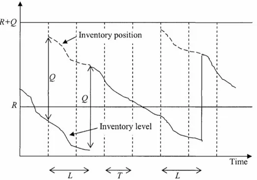
3.2 An (R, Q) policy

With an (R, Q) policy, the inventory position (IP) is observed. When the inventory position declines to (or below) the reorder point (R), a batch quantity of size (Q) is ordered. If the Inventory position is exceedingly below the reorder point, it may be necessary to order a multiple of the batch quantity Q in order to get above R. To further illustrate this process, Figure 1 below illustrates the behaviour of an (R, Q) policy with periodic review and continuous demand. (Ibid.)

Figure 1. Illustration of (R, Q) policy with period review and continuous demand. (Axsäter, 2006)

A natural question to ask is whether there exists a policy better than the described (R, Q) policy. Axsäter, (2006) elaborates that in most situations for singe-echelon inventory systems, especially for situations with low to no ordering cost and fixed batch quantities, the (R, Q) policy is better to use. An alternative would be to replace the fixed quantity Q by always ordering up to a fixed inventory position. Such a policy is however not necessarily optimal when dealing with service constraints. Section 6.4 provides a further motivation as to why the (R, Q) policy has been deemed appropriate to model the current system by.

(27)

15

3.3 Stochastic demand distribution

In practice, the demand during a certain time is nearly always a nonnegative integer, i.e. it is a discrete stochastic variable. In general, for products with low demand, a discrete demand model is suitable to use. However, for products with a higher demand, a continuous demand approximation may be convenient. (Axsäter, 2006)

When modelling demand as continuous distribution, the most common distribution to use is the normal distribution. From the Central Limit Theorem (CLT), under general conditions, a sum of many independent, random variables will have a distribution that is approximately normally distributed (Blom, Enger, Englund, Grandell & Holst, 2005). If the demand in different time increments is mutually independent, and the lead time is the sum of time increments, an approximation can be made. According to CLT, the lead time demand can be approximated as normally distributed - given that the lead time is long enough. However, a problem with the normal distribution is that there is always a small probability for negative demand (Axsäter, 2006). Axsäter (2011) discusses that even lead time demand as low as 10 units, could be modelled successfully with a normal

approximation as the distribution is very robust. Tyworth & John (1997) further elaborates on this subject and argues that a model with normally distributed demand is very robust when calculating costs as well as service levels.

Given the mean and standard deviation of the demand during a specific time, a unique normal distribution can always fit into these kinds of parameters. A standardised normal distribution with a mean µ and standard deviation 𝜎 has the following density:

𝜑(𝑥) = 1 𝜎√2𝜋𝑒

−(𝑥−𝜇)_2𝜎22_{, −∞ < 𝑥 < ∞} _(3.3)

(Blom et. al., 2005)

As the demand in different time increments is mutually independent, the lead time demand can be seen as the sum of these time increments. Moreover, according to CLT, the lead time demand can be approximated as normally distribution given that the lead time is long enough.

(28)

16

3.4 Cost aspects to consider

This section will explain the different cost aspects to consider when constructing an inventory policy, such as: holding costs, ordering costs, backorder cost.

3.4.1 Holding cost

When holding stock there is an opportunity cost for tied up capital in inventory. In principle, holding cost should be similar to the return of an alternative investment. However, the return is not with all certainty expected to be equal to the holding cost. This is due to financial risks associated with alternative investments that need to be taken into account. The holding cost per unit and time unit is usually determined as a percentage (κ) of the unit value. This percentage is then multiplied with the variable replenishment cost per unit (C):

ℎ = 𝜅 ∗ 𝐶 (3.4)

(Axsäter, 2006; Hadley & Whitin, 1963):

This percentage can’t be allocated to all items, hence is product specific. For instance, computers should have high holding cost because of obsolescence. It is common that the percentage is considerably higher than the interest charged by banks (Axsäter, 2006). As Berling (2005) describes the holding cost (h), or carrying cost, it is the cost of carrying one unit of inventory for one unit of time. In accordance with the influential work of La Londe & Lambert (1975), the holding cost can be divided into four major cost components:

● Capital cost ● Storage space cost ● Inventory service cost ● Inventory risk cost

Occasionally, the last three mentioned components are viewed as one and then indicated as out-of-pocket holding cost. The inventory cost risk is associated with a decrease in the value of the inventory, because of changes in the goods’ physical attributes. For instance, the stored goods could be affected by change in fashion, deterioration etc. However, this

(29)

17

risk does not involve costs in association with financial risk i.e. the change in the value of the inventory in relation to the growth of the economy. (Berling, 2005)

3.4.2 Ordering cost

Ordering costs are often associated with fixed costs. Set up cost is synonymous with order cost, with the latter being more frequently used in manufacturing environments. This ordering cost must be weighed against the expected holding cost when determining the order/batch quantity. Ordering costs are typically used when the order is placed at an outside supplier. The costs that are included in ordering costs are clerical of:

● Preparing ● Monitoring ● Realising

● Receiving the order

Additionally, ordering costs frequently includes the costs of the physical handling of goods upon arrival and inspections. (Berling, 2005)

3.4.3 Backorder cost

In the event that demanded items cannot be delivered due to shortage, various costs may be incurred. A customer might be willing to wait for the product. Resulting in costs such as extra administration, discount for late delivery, transportation and handling to be incurred. However, if the customer is not willing to wait, the sale is considered lost and the contribution of the sale is subsequently also considered lost. As shortage and backorder costs are often hard to quantify in practice, it is common to replace the shortage costs with an adequate service level. (Axsäter, 2006)

3.4.4 Service level

In practice, the reorder point is often determined by either taking the backorder costs into consideration or by setting a service level constraint. In practice it is often regarded as easier to specify a service level. The three common service level definitions are:

𝑆1 = 𝑝𝑟𝑜𝑏𝑎𝑏𝑖𝑙𝑖𝑡𝑦 𝑜𝑓 𝑛𝑜 𝑠𝑡𝑜𝑐𝑘𝑜𝑢𝑡 𝑝𝑒𝑟 𝑜𝑟𝑑𝑒𝑟 𝑐𝑦𝑐𝑙𝑒

(30)

18

𝑆3 = "𝑟𝑒𝑎𝑑𝑦 𝑟𝑎𝑡𝑒" − 𝑓𝑟𝑎𝑐𝑡𝑖𝑜𝑛 𝑜𝑓 𝑡𝑖𝑚𝑒 𝑤𝑖𝑡ℎ 𝑝𝑜𝑠𝑖𝑡𝑖𝑣𝑒 𝑠𝑡𝑜𝑐𝑘 𝑜𝑛 ℎ𝑎𝑛𝑑

S1 can be interpreted as the probability that an order arrives in time, i.e., before the stock

on hand is finished. It is a service level commonly used in practice. However, a major weakness is that S1 does not take the batch quantity into consideration. The fill rate (S2)

and ready rate (S3) are more complex to work with. Although, they will most often

provide a more accurate description of the customer service level that the company measures. In this case the fill rate has been chosen to best describe the situation of the case company. (Ibid.)

3.5 Batch quantity

The classical Economic Order Quantity (EOQ) formula is one of the simplest and most well-known in the area of inventory control and lot sizing. The model is based on the following assumptions:

● Demand is constant and continuous

● Ordering and holding costs are constant over time ● The batch quantity does not need to be an integer ● The whole batch quantity is delivered at the same time ● No shortages are allowed

The relevant costs are the costs which varies with the batch quantity Q e.g. the holding cost h and the ordering cost A. With the demand d the resulting cost function can be obtained as:

𝐶 =𝑄_{2 ∗ ℎ +}𝑑_{𝑄 ∗ 𝐴} (3.5) This resulting cost function is convex and by solving the cost minimisation problem with respect to Q we obtain the economic order quantity as:

𝑄∗_{= √}2 ∗ 𝐴 ∗ 𝑑

ℎ (3.6)

(31)

19

𝐶∗_{= √2𝐴𝑑ℎ} _(3.7)

And can finally see how important the optimal order quantity is by combining (3.5), (3.6) and (3.7) into:

𝐶

𝐶∗=1_{2 ∗ (}_𝑄𝑄∗+𝑄 ∗

𝑄 ) (3.8)

From which it can be observed that the cost increase is a simple function of Q/Q*, which varies very little even with large deviations from the optimal order quantity.

3.6 Reorder point

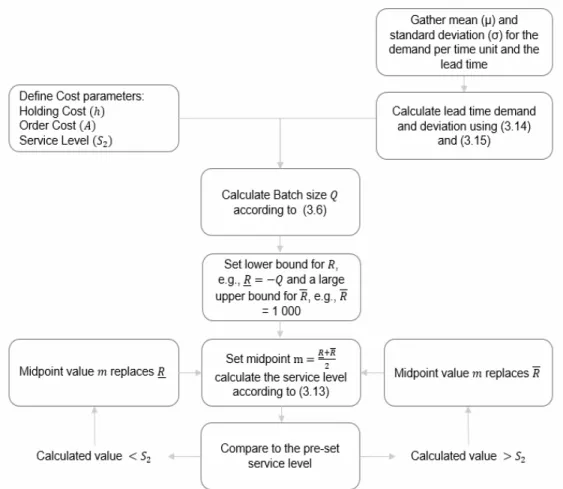
In order to determine the reorder point, we must first choose a suitable demand model and review model. As mentioned in section 3.3, according to the CLT, the lead time demand data should follow a continuous normal distribution, given that the lead time is long enough. This hypothesis will be further tested in section 6.2. Regarding the choice of review model, is has been deemed appropriate to use continuous review. However, this is an approximation of the current process. As the review window of the case company is weekly, it can be approximated to follow a continuous review by adding half a review period to the total lead time. With a review period (T) of one week, in best case scenario, the order will be placed if the inventory position is observed to exactly hit the reorder point. In contrast, the worst case scenario is that the inventory position will not be observed to have surpassed the reorder point until T time units later. Thus, by assuming equal probability of observing an inventory position below R during the review period, we will on average place an order 𝑇/2 time units after the inventory position has surpassed the reorder point. The lead time can then be expressed as 𝐿̃ = 𝐿 +𝑇₂. The reorder point will be determined by evaluating what reorder point is fulfilling a specific fill rate, denoted as 𝑆2 in section 3.4.4

When dealing with normally distributed demand, we assume that the inventory position is uniformly distributed on the interval [R, R+Q]. Now, consider an arbitrary time t when a system is in steady state. Define 𝐼𝑃(𝑡) as the inventory position an arbitrary time 𝑡, and 𝐷(𝑡, 𝑡 + 𝐿) the lead time demand over the lead time 𝐿 between time 𝑡 and 𝑡 + 𝐿, then the inventory level at time 𝑡 + 𝐿 can be defined as:

(32)

20

𝐼𝐿(𝑡 + 𝐿) = 𝐼𝑃(𝑡) − 𝐷(𝑡, 𝑡 + 𝐿) (3.9) Next, we assume that the demand in mutually exclusive time periods is independent. For normally distributed demand and constant lead time, let 𝜇′ _{= 𝜇 ∗ 𝐿 and 𝜎}′ _{= 𝜎 ∗ √𝐿 ,}

denote the mean and standard deviation of the lead time demand. For continuously, normally distributed demand, we can then obtain the inventory level distribution function as:

𝐹(𝑥) = 𝑃(𝐼𝐿 ≤ 𝑥) =_{𝑄 ∗ ∫}1 𝑅+𝑄[1 − 𝛷 (𝑢 − 𝑥 − 𝜇_𝜎_′ ′)]

𝑅 𝑑𝑢 (3.10)

Given the inventory position 𝑢 at an arbitrary time 𝑡, the inventory level at time 𝑡 + 𝐿 is less than or equal to 𝑥 if the lead time demand is 𝑢 − 𝑥 (Axsäter, 2006). Next, the loss function, i.e., the amount of shortages that occur in one cycle, is defined as:

𝐺(𝑥) = ∫ (𝑣 − 𝑥) ∗ 𝜑(𝑣)𝑑𝑣𝑖𝑛𝑓

𝑥 = 𝜑(𝑥) − 𝑥 ∗ (1 − 𝛷(𝑥)) (3.11)

By using that 𝐺′_{(𝑥) = Φ(x) − 1 (3.10) can be reformulated as:}

𝐹(𝑥) = (𝜎_{𝑄 ) [𝐺 (}′ 𝑅 − 𝑥 − 𝜇_𝜎_′ ′) − 𝐺 (𝑅 + 𝑄 − 𝑥 − 𝜇_𝜎_′ ′)] (3.12) Furthermore, for continuous review, 𝑆2= 𝑆3 and the service level can be expressed as

the probability of positive stock on hand, which can be denoted as:

𝑆2= 𝑆3= 1 − 𝐹(0) = 1 − (𝜎 ′ 𝑄 ) [𝐺 ( 𝑅 − 𝜇′ 𝜎′ ) − 𝐺 ( 𝑅 + 𝑄 − 𝜇′ 𝜎′ )] (3.13)

For a given service level, the reorder point can be calculated by using a bisection search. Starting with a lower bound for 𝑅, e.g., 𝑅 = −𝑄 and an upper bound of 𝑅. Next, 𝑅 =

𝑅+𝑅

2 is considered. If the resulting service level is too low 𝑅 can replace 𝑅 and otherwise it

(33)

21

3.7 Stochastic lead times

Liao & Shyu (1991) define lead times as the time from when an order has been placed, until it is has arrived in the warehouse and is ready to satisfy demand. According to Axsäter (2006), the most common type of stochastic lead time is sequential deliveries, i.e. orders cannot cross in time. While the stochastic lead times may be dependent on the previous demand due to congestions in the supply system - the demand perceived after the order has been placed will not affect the lead time. The distribution of the demand during a stochastic lead time can be replaced by a normal distribution with correct mean and variance. We denote the mean and standard deviation as (µ) and (σ) respectively. We obtain the mean of the stochastic lead time demand D during the as:

𝐸(𝐷) = 𝜇 ∗ 𝐸(𝐿) (3.14) For a given 𝐿, 𝐸(𝐷(𝐿))2= 𝜎2_{+ (𝜇 ∗ 𝐿)}2_{, the variance of D can be determined as:}

𝑉𝑎𝑟(𝐷) = 𝜎2_{𝐸(𝐿) + 𝜇}2_{∗ 𝑉𝑎𝑟(𝐿)} _(3.15)

By setting 𝜇′ _{= 𝐸(𝐷) and 𝜎}′_{= √(𝑉𝑎𝑟(𝐷)) we can, as an approximation, use}

expressions for constant lead times such as in section 3.6.

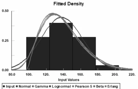
3.8 Distribution fitting and analysis of input data

The first step in order to construct and adequate inventory policy and forecasting model, is to determine the distribution of the demand. In order to evaluate what distribution to construct a model by, the ExtendSim-tool Stat::Fit has been used. It must be noted, however, that the test can in no way prove the hypothesis that a certain set of data points follow a particular distribution. Instead, the tested hypothesis is that the inspected data points are independent samples from a theoretical probability distribution. If the hypothesis is rejected, it can be concluded that the theoretical distribution is a not good representation of the data set. However, failure to reject the hypothesis does not imply that the hypothesis is true. There might be several candidate theoretical distributions that could be considered a good fit for the data set.

(34)

22

Two of the most well-known goodness of fit tests are the chi-square test and the Kolmogorov-Smirnov (KS) test, which are both used by the Stat::Fit tool. Specific definitions of both tests as well as examples and can be found in Laguna & Marklund (2013).

3.9 Forecasting

There are mainly two reasons why inventory control systems require products to be ordered before customers demand them. Firstly, there is almost always a lead time between the time of ordering and time of delivery. Secondly, depending on the ordering costs, it is usually necessary to order in batches rather than single units. Hence, it is vital to forecast the future demand. The demand forecast is an estimated average of the future demand for a specific period of time. However, it’s not sufficient to only estimate the average demand. There is a necessity to determine how uncertain the forecast is. If there is a great uncertainty in the forecast, there might be a need for a larger safety stock.

Therefore, an analysis of the deviations in the forecast is also needed. (Axsäter, 2006)

3.9.1 Forecasting approaches

According to Axsäter (2006), there are generally two types of forecasting methods that are suitable for inventory control. Typically, these forecast approaches concerns a relatively short time horizon. It’s seldom necessary to look more than a year ahead. The two type of approaches are:

● Extrapolation of historical data ● Forecasts based on other factors

Forecast that is based on prior demand data, is extrapolated and based on statistical methods. Extrapolation is the most important and commonly used approach to acquire forecasts over shorter horizons. Forecasts based on other factors is used when the demand of an item is dependent on e.g. another item(s), sales campaigns and more. (Axsäter, 2006)

3.9.2 Demand models

As mentioned before, extrapolation of historical data is the most commonly used approach for demand-based forecasting method within inventory control. However, to

(35)

23

find an appropriate technique, we need to model the stochastic demand. Some examples of these models are; constant, trend and trend-seasonal models (Axsäter, 2006)

3.9.2.1 Constant model

The simplest demand model is constant. This means that demand in different periods are represented by independent random deviations from an average. This average is assumed to be relatively stable over time in comparison to the random deviations. To represent a constant model, the following notations need to be introduced:

𝑥𝑖= 𝑑𝑒𝑚𝑎𝑛𝑑 𝑖𝑛 𝑝𝑒𝑟𝑖𝑜𝑑 𝑡,

𝑎 = 𝑎𝑣𝑒𝑟𝑎𝑔𝑒 𝑑𝑒𝑚𝑎𝑛𝑑 𝑝𝑒𝑟 𝑝𝑒𝑟𝑖𝑜𝑑 (𝑎𝑠𝑠𝑢𝑚𝑖𝑛𝑔 𝑡ℎ𝑎𝑡 𝑖𝑡 𝑣𝑎𝑟𝑖𝑒𝑠 𝑣𝑒𝑟𝑦 𝑠𝑙𝑜𝑤𝑙𝑦), 𝜀𝑖= 𝑖𝑛𝑑𝑒𝑝𝑒𝑛𝑑𝑒𝑛𝑡 𝑟𝑎𝑛𝑑𝑜𝑚 𝑑𝑒𝑣𝑖𝑎𝑡𝑖𝑜𝑛𝑠 𝑤𝑖𝑡ℎ 𝑚𝑒𝑎𝑛 𝑧𝑒𝑟𝑜.

With these notations, a constant demand model for period t can be represented as

𝑥𝑡 = 𝑎 + 𝜀𝑖 (3.16)

There are many products that can be well represented by a constant model, particularly for products that are in their mature stage of its product life cycle and used regularly. In cases where trends and seasonalities are not expected, it is reasonable to assume a constant model. (Ibid.)

3.9.2.2 Trend model

In cases where the demand is assumed to decrease and increase systematically, it is possible to extend the constant model by considering a linear trend. Let

𝑎 = 𝑎𝑣𝑒𝑟𝑎𝑔𝑒 𝑑𝑒𝑚𝑎𝑛𝑑 𝑖𝑛 𝑝𝑒𝑟𝑖𝑜𝑑 0,

𝑏 = 𝑡ℎ𝑒 𝑠𝑦𝑠𝑡𝑒𝑚𝑎𝑡𝑖𝑐 𝑡𝑟𝑒𝑛𝑑 𝑡ℎ𝑎𝑡 𝑖𝑛𝑐𝑟𝑒𝑎𝑠𝑒𝑠 𝑜𝑟 𝑑𝑒𝑐𝑟𝑒𝑎𝑠𝑒𝑠 𝑝𝑒𝑟 𝑝𝑒𝑟𝑖𝑜𝑑 (𝑎𝑠𝑠𝑢𝑚𝑖𝑛𝑔 𝑖𝑡 𝑣𝑎𝑟𝑖𝑒𝑠 𝑠𝑙𝑜𝑤𝑙𝑦)

The trend model can be modelled as followed:

𝑥𝑡 = 𝑎 + 𝑏𝑡 + 𝜀𝑖 (3.17)

During stages such as initial growth stages and phase-out stages in a product life cycle, it is natural to assume that the demand follows a positive respectively negative trend model. (Ibid.)

(36)

24

3.9.2.3 Trend-seasonal model

To describe a trend-seasonal model, the following notation needs to be introduced:

𝐹𝑡= 𝑠𝑒𝑎𝑠𝑜𝑛𝑎𝑙 𝑖𝑛𝑑𝑒𝑥 𝑖𝑛 𝑝𝑒𝑟𝑖𝑜𝑑 𝑡 (𝑎𝑠𝑠𝑢𝑚𝑖𝑛𝑔 𝑡ℎ𝑎𝑡 𝑖𝑡 𝑣𝑎𝑟𝑖𝑒𝑠 𝑠𝑙𝑜𝑤𝑙𝑦)

The seasonal index indicates how the demand in period t is expected to change due to seasonal variations. For instance, 𝐹𝑡 = 1,2 means that demand in period t is expected to

become 20 percentage higher because of seasonal variations. The trend-seasonal demand model can be modelled as

𝑥𝑡 = (𝑎 + 𝑏𝑡)𝐹𝑡+ 𝜀𝑖 (3.18)

Here it is assumed that the variations of the seasons increase and decrease proportionally with the changes in the level of the demand series. This is in many cases a reasonable assumption. An alternative assumption to this is seasonal demand variations being additive. There are many products that have seasonal demand variations. For instance, demand for ice cream increases during the summer. However, a seasonal model is only essential if the demand follows the same pattern year after year. (Ibid.)

3.9.3 Choosing demand model

By studying the three demand models, the trend model is more general than the constant model. Consequently, the trend-seasonal model is even more general than the trend model. Even though a more general model seems to be more advantageous, it is not necessarily the case. Because a more general demand model covers a wider range of demand classes, more parameters need to be estimated. It might be quite difficult to determine accurate estimations of the parameters, especially if the independent deviations are relatively large. Thus, it might be more efficient to use a simpler demand model with fewer parameters. Therefore, a use of a simpler demand model, with fewer parameters, is more efficient. Moreover, it is worth noting that the independent deviations, 𝜀𝑡, can’t be

forecasted. Hence, the best forecast for 𝜀𝑡 is always zero. Consequently, if the

independent deviations are relatively large, there is no possibility to avert large forecast uncertainties. (Ibid.)

A practical issue when using demand models, is that it is often very difficult to obtain demand data. The reason is that usually only sales are recorded. When using historical sales data instead of historical demand data for forecasting, some significant errors might

(37)

25

occur in situations where larger portions of the total demand is lost because of shortages. (Ibid.)

The basic forecasting models in the following sections - moving average, simple

exponential smoothing and exponential smoothing with trend - are commonly used and are in general suitable techniques for most items. (Ibid)

3.9.4 Moving average

The moving average technique is performed by taking the average over the N most recent demands. Here it is assumed that the underlying structure is described as a constant model. Due to the independent deviations 𝜀𝑡 can’t be predicted, the average demand

𝑎 needs to be estimated. In the case of 𝑎 being completely constant, the best estimate would be the average of all observations 𝑥𝑡. However, if 𝑎 vary slowly, then the most

recent values of 𝑥𝑡 are the most relevant to consider. To present a moving average model,

the following notations need to be introduced:

â𝑡= 𝑒𝑠𝑡𝑖𝑚𝑎𝑡𝑖𝑜𝑛 𝑜𝑓 𝑎 𝑎𝑓𝑡𝑒𝑟 𝑑𝑒𝑚𝑎𝑛𝑑 𝑜𝑏𝑠𝑒𝑟𝑣𝑎𝑡𝑖𝑜𝑛 𝑖𝑛 𝑝𝑒𝑟𝑖𝑜𝑑 𝑡

𝑥 𝑡,𝜏= 𝑓𝑜𝑟𝑒𝑐𝑎𝑠𝑡 𝑓𝑜𝑟 𝑝𝑒𝑟𝑖𝑜𝑑 𝜏 > 𝑡 𝑎𝑓𝑡𝑒𝑟 𝑑𝑒𝑚𝑎𝑛𝑑 𝑜𝑏𝑠𝑒𝑟𝑣𝑎𝑡𝑖𝑜𝑛 𝑖𝑛 𝑝𝑒𝑟𝑖𝑜𝑑 𝑡

Hence, the moving average can be described as:

𝑥̂𝑡,𝜏= â𝑡 =(𝑥𝑡+ 𝑥𝑡−1+ 𝑥1−2_𝑁 + ⋯ + 𝑥𝑡−𝑁+1) (3.19)

Due to assuming a constant demand model, the forecast demand for any value 𝜏 > 𝑡 is the same. The value of N depends on how slowly it is estimated that 𝑎 will vary, as well as the size of the stochastic deviations of 𝜀𝑡. In the case of 𝑎 varying slowly and the

stochastic deviations are relatively large, a higher value of N is more adequate. This is done in order to limit the influence of the stochastic deviations. In the other case, if the stochastic deviations are relatively small and 𝑎 varies rapidly, a smaller value of N is preferable. (Ibid.)

3.9.5 Exponential smoothing

Exponential smoothing, also known as simple exponential smoothing, is another forecasting method. Assuming a constant demand model, we strive to determine the

(38)

26

average demand in the first period. To update the procedure of the forecast, in a specific period, a linear combination of the most recent demand and previous forecast is used. Resulting in the following model:

𝑥̂𝑡,𝜏= â𝑡 = (1 − 𝛼)â𝑡−1+ 𝛼𝑥𝑡 (3.20)

Where 𝜏 > 𝑡 and 𝛼 = 𝑠𝑚𝑜𝑜𝑡ℎ𝑖𝑛𝑔 𝑐𝑜𝑛𝑠𝑡𝑎𝑛𝑡 (0 < 𝛼 < 1)

When 𝛼 = 0, the forecast does not get updated. Consequently, when 𝛼 = 1, the most recent demand is chosen for the forecast. In monthly forecast updates, a typical value for the smoothing constant is between 𝛼 = 0,1 and 𝛼 = 0,3 (Axsäter, 2006). According to Silver, Pyke & Peterson (1998) a larger value of 𝛼 = 0,3 in simple exponential smoothing procedures should raise the question of validity of the assumed underlying model. In such cases, it should be considered to use an exponential smoothing with trend model instead.

3.9.6 Exponential smoothing with trend

An updated version of exponential smoothing is that the demand also follows a trend. In this case, two parameters need to be estimated - â𝑡 and 𝑏̂𝑡. As in the constant model, â𝑡

denotes the average demand per period while 𝑏̂𝑡 denotes the trend that is the systematic

decrease or increase in demand per period. As mentioned before, the independent deviation, 𝜀𝑖, cannot be predicted. There exist different methods for estimating â𝑡 and 𝑏̂𝑡.

The considered approach was proposed by Holt (2004):

â𝑡 = (1 − 𝛼) ∗ (â𝑡−1+ 𝑏̂𝑡−1) + 𝛼𝑥𝑡 (3.21)

𝑏̂𝑡 = (1 − 𝛽) ∗ 𝑏̂𝑡−1+ 𝛽 ∗ (â𝑡− â𝑡−1) (3.22)

The smoothing constants and β are values between 0 and 1. Furthermore, the “average” â𝑡coincide to period t where the demand has been observed. For the future period, i.e.

𝑡 + 𝑘, the forecast can be obtained by:

𝑥̂𝑡,𝑡+𝑘 = â𝑡+ 𝑘 ∗ 𝑏̂𝑡 (3.23)

Note that the trend could either be positive or negative. The purpose of exponential smoothing with trend is to follow systematic linear changes in demand more accurately.

(39)

27

When the smoothing constants, and β, are relatively large, the forecast reacts more quickly to changes. However, this also makes the forecast more sensitive to stochastic deviations. When the forecast is updated monthly, some conventional values for the smoothing constants are 𝛼 = 0,2 and 𝛽 = 0,05. Additionally, when initiating the forecast, it is plausible to assume the trend 𝑏̂0= 0. (Axsäter, 2006)

3.10 Human judgement

When deciding an adequate demand model, it is mostly based on historical data. However, in some cases, human judgement is more advisable to use for estimating the future

demand. For instance, in situations when known factors will affect the future demand, although haven’t affected the previous demand. Thus, forecasting systems should be designed so both automatic and manual forecast can easily be used. Cases where manual forecasting is suitable is when factors such as; sales promotions, price changes, new products, conflicts that influence the demand or new regulations influence the demand. (Ibid.)

3.11 Forecast errors

The following section describe forecast errors and how they should be updated. In addition, the section contains how manual forecasting should be considered.

3.11.1 MAD and standard deviation

In addition to estimating the mean of the future demand, it is also necessary to know how uncertain the forecast is - i.e. the size of the forecast errors. This is necessary for

determining a suitable safety stock. Commonly, variations are described as the variations around the mean through the standard deviation. By letting X be a stochastic variable with the mean, 𝑚 = 𝐸(𝑋), the standard deviation σ is defined as:

𝜎 = √𝐸(𝑋 − 𝑚)2 _(3.24)

Another measure of variability is the Mean Absolute Deviation (MAD) which was originally recommended for its simple computational practices. MAD describes the expected value of the absolute deviation from the mean and defined as:

(40)

28

𝑀𝐴𝐷 = 𝐸 |𝑋 − 𝑚 | (3.25) (Ibid.)

According to Silver, Pyke & Peterson (1998), MAD can also be described as:

𝑀𝐴𝐷 = ∑|𝑥𝑡− 𝑥̂_𝑛𝑡−1,𝑡|

𝑛

𝑡=1

(3.26) The original reason for its use was its computational simplicity. However, if the errors are assumed to be normally distributed, the standard deviation can be obtained. Standard deviation and MAD give similar picture of how the demand varies around the mean. In the case of assuming the forecast errors being normally distributed, which is very common, the relation between MAD and σ is described as:

𝜎 = √𝜋_{2 ∗ 𝑀𝐴𝐷 ≈ 1,25 ∗ 𝑀𝐴𝐷} (3.27) The relation above is commonly used within forecasting. Even in cases when it is less reasonable that the errors are normally distributed (Axsäter, 2006). However, according to Silver, Pyke & Peterson (1998), using a normal distribution for forecast errors are

recommended for three reasons. Firstly, empirically the normal distribution often gives a better fit to data than many other suggested distributions. Secondly, if the lead time is long and forecast errors in several periods are added, a normal distribution would be expected through the Central Limit Theorem. Lastly, the normal distribution leads to manageable and analytical results.

3.11.2 Updating MAD

Let MADt denote the estimation of MAD after period 𝑡. At the end of period 𝑡 − 1, a

forecast for period 𝑡, 𝑥 _{𝑡−1,𝑡} can be obtained from the forecasting system. This could be regarded as a “mean” for the stochastic demand in period 𝑡, 𝑥𝑡. Although, this is not

always accurate due to systematic errors in the forecast that frequently occurs. After period 𝑡, the value 𝑥𝑡 is obtained and consequently the absolute deviation from the

“mean”, |𝑥𝑡− 𝑥 𝑡−1,𝑡|. Generally, it is assumed that the absolute deviations can be

observed as independent, stochastic deviations from the mean that varies somewhat slowly. Following a constant model in accordance to (3.16), MADt can for example be

(41)

29

updated by exponential smoothing. The forecast for the MADt at the end of period 𝑡 is

described as:

𝑀𝐴𝐷𝑡 = (1 − 𝛼) ∗ 𝑀𝐴𝐷𝑡−1+ 𝛼 ∗ |𝑥𝑡− 𝑥̂𝑡−1,𝑡| (3.28)

where 0 < 𝛼 < 1 is the smoothing constant. Note that this constant is not necessarily the same as in exponential smoothing but often it is used in a similar fashion. Due to the absolute deviation frequently varies a lot, the smoothing constant is chosen relatively small. (Ibid.)

Alternatively, to (3.28), is to update the MADt as a moving average (3.19). When MADt

has been determined, the standard deviation can be calculated in similar way as in (3.27):

𝜎 = √𝜋_{2 ∗ 𝑀𝐴𝐷}𝑡 ≈ 1,25 ∗ 𝑀𝐴𝐷𝑡 (3.29)

(Ibid.)

3.11.3 Manual forecast

The previously discussed forecasting models have been related to extrapolating historical data. However, in some cases, these forecasting techniques are less suitable to use. For instance, in cases where factors affecting the future demand, e.g. promotions, has not been observed in historical demand. In these situations, it is appropriate to let manual interactions with the forecast be conducted rather than automatic ones. Hence,

forecasting systems should be designed so that switching between automatic and manual forecasts can be easily managed. (Ibid.)

Usually, the use of manual forecasts is conducted for a number of items during a relatively short time span. Some cases were manual forecasts can be considered are:

● Sales campaigns

● Conflicts that affect the demand ● Changes in price

● Newly introduced products without historical data ● New competitive products in the market

(42)

30

A frequent complication with manual forecasts is the systematic errors that occur due to optimistic or pessimistic beliefs by the people that forecasts. Resulting in over-

respectively under-procurement of stock. (Ibid.)

3.11.4 The problem of overfitting

According to Kuhn & Johnson (2013), there exists many techniques that can follow the structure of a set of data very well. In a matter of fact, it follows the data so accurately that the applied model correctly predicts every sample. Furthermore, in addition to following the general patterns of the data, the model also has the capability to follow each

characteristic of the sample’s unique noises - i.e. some of the residual variations have been extracted as if they represent the underlying model structure. These types of models are said to be overfitted and will generally have poor accuracy when forecasting a new sample. According to Liu (2000), overfitting normally occurs when including too many regressors in a model or using more complicated non-linear models to estimate a linear or non-linear relationship.

3.12 Updating Order quantities and Reorder points

In earlier sections of the thesis, various techniques for forecasting and determining batch quantities and reorder points have been described. These techniques can be implemented into an inventory control system. Forecasts are usually updated in periods. Generally, it is practical to update the reorder points and batch quantities at the same time as the forecast is updates. Let 𝑡𝐹 denote the forecast period which can be set differently - days (𝑡𝐹= 30),

months (𝑡𝐹 = 1), years (𝑡𝐹 = 1/12) etc. Generally, it is favourable to use the same time

unit in all inventory control calculations. Usually, forecasts are updated by either exponential smoothing (Section 3.9.5) or exponential smoothing with trend (Section 3.9.6).

In order to determine the reorder point, the distribution of the lead time demand has to be determined. By letting μ’ and σ’ be the mean and average of the lead time demand after the forecast update, the simple exponential smoothing and moving average is:

𝜇’ =â_𝑡𝑡

𝐹∗ 𝐿 (3.30)

(43)

31 𝜇’ = 𝑔(𝐿) (3.31) 𝑔(𝐿) = (â +𝑏̂_{2 ) ∗}𝑡 _𝑡𝐿 𝐹+ 𝑏̂𝑡∗ 𝐿2 2 ∗ 𝑡𝐹2 (3.32)

The standard deviation is described as:

𝜎’ = 𝜎 ∗ 𝐿𝑐_{= √}𝜋 2 ∗ 𝑀𝐴𝐷𝑡∗ ( 𝐿 𝑡𝐹) 𝑐 (3.33) Where the parameter𝑐 = 0,5 if the forecast errors are assumed to be independent during different time periods. This is considered a standards assumption, in which the parameter 𝑐always is within the interval [0,5 ; 1].

The batch quantity is most commonly updated by demand per time unit ( ), holding cost rate per time unit (h) and ordering cost (A), similar as in section 3.5:

𝑄 = √2 ∗ 𝐴 ∗ 𝜇_ℎ (3.34) (Axsäter, 2006).

Furthermore, it is not common to consider stochastic variations in lead times. A reason for this is the difficulty to determine the distribution of the lead time. However, if the lead time variations are known and deliveries are sequential, it is appropriate to utilize the approximation seen in section 3.7. With the newly updated mean and standard deviation for the lead time, the batch quantities and reorder points can be updated as described in section 3.5 and 3.6 respectively.

3.13 Performance evaluation and aggregation

The general purpose of an inventory control system is to reduce ordering and holding cost while still maintaining customer satisfaction. Therefore, it is essential to be able to evaluate the performance continuously. Evaluating performance is needed for the availability of adjusting the control when different changes in operations occurs and creating motivation

(44)

32

for efficient application. The performance evaluation should consider several important aspects; e.g. costs regarding tied up capital in inventories and ordering costs or service levels. Normally, it’s not difficult to decide proper performance measures. The most difficult objective is to choose the level of aggregation for measurement. Due to often hundreds or thousands of items, it is not practical to follow individual items separately. Neither is it suitable to aggregate all items. It is advantageous to aggregate products that are similar and having similar inventory control. The evaluation of the performance should primarily be aggregated to relatively large groups and afterwards, if required, be divided into smaller groups. Additionally, it is important to be aware of potential measurement errors and take them into account when interpreting the results. (Ibid.)

(45)

33

4. Background to LSBolagen

The following section gives an overview of the case company, particularly with regards to its products markets, customers and supply network.

4.1 The company

LSBolagen is, as previously mentioned, distributing a wide range of products served in European countries. The company can be divided into four business units:

Administration, Sales, Purchasing, Marketing and Economy. With the current business model, products are procured from suppliers in both Europe and Asia, with the largest suppliers operating in East Asia.

This study will focus on the key products of the two biggest suppliers located in China. Further explanation of the characteristics of the products analysed, as well as the different markets and supplier network, will be provided in the following sections.

4.2 Products

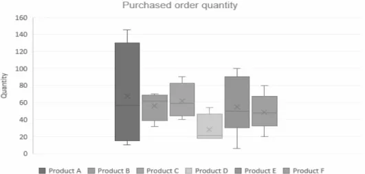
The products the company is selling are mainly high-end retail products of different types. The six products chosen for evaluation are from two highest grossing segments.

Furthermore, these six products are among the highest turnovers within their specified category and have been chosen to be evaluated by the company. The products will henceforth be referred to as Product A-F, where products A-C are from one segment and products D-F from another. These products are mostly bought by customers by one piece at a time, but in some cases more than one per order.

4.3 Market and customers

The customers the company serves are mainly private consumers and companies interested in these retail products for long-term use. Additionally, some companies buy these products during events and are consequentially bought in larger quantities. The customers are, as mentioned, mainly resident in the Nordic countries, the UK, Germany and France. The different customer segments’ geographical areas will not be analysed individually. The main focus is to develop an inventory policy for the warehouse in Sweden, which serves to all these customers.

(46)

34

4.4 Supply network

The company’s suppliers for these six products are mainly located in China. The

purchased products are then shipped and transported to either the company’s warehouse in Sweden or to their satellite warehouse in the UK. These products are produced at the supplier when the case company makes an order. Hence, upon orders from the company, the production starts and are then transported to designated destination in either Sweden or the UK. The two suppliers analysed in this report are both situated in eastern Asia. Due to the production and long transportation time from China to Europe, the lead time is several months long.

Forming an Inventory Control Policy and Forecasting Model for an E-Commerce Company