By
N. Djordjevic, W. Ehrman, and G. Swanson
Principal Investigator: Elmar. R. Reiter
Technical Paper No. 105
Department of Atmospheric Science
Colorado State University
Fort Collins, Colorado
FURTHER STUDIES OF DENVER AIR POLLUTION by N. Djordjevic W. Ehrman G. Swanson
Principal Investigator: Elmar R. Reiter
This Report was Prepared with Support from Grant 5 ROI AP 00216-03 with the
Department of Health, Education and Welfare
Department of Atmospheric Science Colorado State University
Fort Collins, Colorado
December 1966
Foreword
by E1mar R. Reiter . . . . Air Trajectories for Studying Denver Air Pollution by N enad Djordj evic . . . • . . • Data Processing Techniques Employed with Denver Air
Pollution
by William Ehrman . • . . . • • . . • . • • . . . Microscopical Analysis of Atmospheric Particulates Found
in Denver Air Pollution
Pages i - ii 1-104 105-108 by Glenda Swanson. . . • . . . • . • . . . • . . • • . . . . 109-146 i
FOREWORD
The Denver Air Pollution Study was authorized in November 1963. The first season of observations could not be started until
the winter of 1964-1965. It was followed by a second observational
season during the winter of 1965 -1966.
Various unforeseen difficulties had to be overcome as the measurement program developed. So, for instance, it was necessary to develop a complete network of COH (coefficient of haze) samplers which, according to original plans, was supposed to be set up and operated by cooperating agencies. A Royco particle counter, acquired under Health, Education and Welfare funding, had to be adapted for field use. The large meteorological network, which was established in support of the air pollution study. required close supervision and a detailed maintenance schedule.
The present report constitutes the preliminary result of analysis work conducted on the large amount of meteorological and pollution data collected during the two pollution seasons men-tioned above. Specific efforts were made to compare the behavior of air pollution patterns during certain episodes, as evident from the COB data, with the quasi -periodic wind regimes over the city of Denver. The phenomenon of the "heat island" was explored in a preliminary way by tracing constant level balloon trajectories, and
by recording vertical temperature gradients in the lowest layers of
the atmosphere by means of wiresondes. Even though it appears
that under conditions of persisting inversions the "heat island'l does not affect horizontal air trajectories to any great extent, more detailed measurements of three-dimensional air motions are desired. Especially for weather conditions in which inversions are briefly penetrated during the noon hours. the air trajectory behavior should be subject to additional investigation.
in the final part of this report. are still in a preliminary stage. From these analyses it appears that the identification of certain "characteristic"
pollutants may be possible. It will be the task of additional
measure-ments. in which pollution sample collection is closely coordinated with detailed meteorological observations, to obtain more definite indiea-' tions of specific sources of pollutants, their relative abundance, and their diffusion over the metropolitan area of Denver.
In the author) s opinion the following problem areas still remain to be challenged:
(a) What is the total "spectrum" of gaseous, liquid, and solid pollutants produced by various sources as a function of time?
(b) How do these pollutants disperse in the vicinity of the source, as well as over wide areas?
(c) How do the various gaseous. liquid, and solid pollutants interact with each other and with the atmosphere and its variable parameters such as moisture. pressure, temperature, radiation, and "natural" trace gases and aerosols?
(d) Detailed consideration of aerosol and pollution chemistry under varying atmospheric conditions is expected to yield !!half-life" estimates of pollutants.
(e) A better understanding of the physical chemistry uf pollu-tants may also yield improved methods of pollution control.
Although the present field study of air pollution in the Denver metropolitan area is not designed to answer these rather sophisticated-,,-yet fundamental--questions. the data collected under this study will
serve as basis of more refined research approaches.
iii
Elmar R. Reiter, Acting Head Department of Atmospheric Science Colorado State University
gradient does exist so that the surface wind field may undergo changes because of the local influence of terrain. Such well-developed and
slowly moving anticyclones are characteristic for a broad scale weather pattern most likely to produce simultaneous occurrence of very low wind speed, pronounced stability. and fog over the continental United States for a few days. causing severe air pollution in many cities (Niemeyer. 1960).
The influence of local topography in such weather situations on the wind regime in the lower layers of the atmosphere (up to about 2,000 feet) is pronounced. In mountain valleys. the phenomenon of a daily wind regime with upslope motion occurs during most of the dc.y-time. During the night, a reversed flow down the valley takes place. It is not the purpose of this report to discuss the theory of mountain and valley winds which has already been given in a comprehensive form by Defant (1951). It will only be mentioned that such circulations are almost an everyday phenomenon over Denver on days with air pollution as will be seen later.
It is a well-known fact that the degree of air pollution depends on the amount of pollutants introduced and on the capability of the air to absorb and disperse this pollution. The latter in turn depends on the vertical structure and on the wind characteristics of the air mass
(Gosline. et al .• 1956).
The vertical structure of an air mass is described by the
verti-cal temperature lapse rate. On the average. the lapse rate. 'Y. is
about. 6°C/100 meters. An air parcel displaced upward will change its temperature dry-adiabatically or pseudo-adiabatically. depending on whether the parcel is unsaturated or saturated with water vapor.
Air stability is usually compared with the dry-adiabatic lapse rate
r
which is loC/100 meters. Thus. at some height the parcel will be
-8-temperature as its environment if 'Y =
r.
These three values of 'Ycharacterize stable, unstable, and indifferent conditions, respectively. When inversions are present, the temperature above a given
place increases with height and 'Y <
r.
If the inversions are strong,as they sometimes are over Denver, 'Y may attain the value of
_90
el
1 00 meters as will be seen later. Therefore, an air parceldisplaced upward will always be colder than its environment. thus indicating stable conditions. Because of this, the possibility for a transport of the polluted air upward is limited.
The wind characteristics of an air mass important for a dis-persion of the pollutants include wind speed and direction as well as the fluctuations of both around the mean values, the latter giving a measure of turbulence. Assuming that the sources of pollutants are constant, the greater the mean wind speed, the less concentrated will the pollutants be downstream from the source. Furthermore, the greater the fluctuations of instantaneous winds around the mean, the stronger the dispersion of pollutants. Neuberger et al. (1956) sum-marized the results of tentative statistical studies of the properties of turbulence and arrived at six major groups of characteristics from which only parts of two particularly relevant groups will be cited:
(l) Turbulent energy is greater in unstable air, smaller in
stable air;
(2) Turbulent energy increases with increasing wind speed as well as with increasing vertical variations of the wind.
Thus, stability and low winds tend to prevent the dispersion of pollutants and may allow the concentration of contaminants to reach high values.
An illustrative description of how pollutants disperse under different stability conditions at the same wind speed is given in Fig. 2. As can be seen, the highest concentration in the plume can be expected in an inversion condition.
-10-In an urban environment, the distribution of the pollution sources together with wind, stability, and topographic conditions may produce a very complicated distribution of pollutants. Further-more, the height, the relative distance and the strength of sources, and the time variability of pollution emission, create exceedingly complex distributions of pollutants over certain observation points within a city. Neiberger (1961) in his theoretical study gave a sche-matic representation of the concentration variations of pollution at the earth's surface as a function of the distance from randomly sized and spaced elevated sources (Fig. 3). From this figure it follows that one may expect a gradual increase of the concentration down-wind, up to the maximum at a certain distance from the first upwind source.
If this model is applied to the Denver area during the days
with low wind speed and inversion of temperature, the highest con-centration would be expected to be in the northern part of the city during the downslope flow and in the southern part during the upslope motion of the air.
A photograph taken from aircraft over Denver show s the polluted mass of air on such a day with inversion and low wind speed (Fig. 4).
Purpose
The primary purpose of this study was to determine the main types of wind flow during the days with air pollution over the Denver metropolitan area. Air pollution was considered as a bulk property of air.
The secondary objective was to gain a knowledge on the sources of pollution and the trajectories of air motion over the Denver metro-politan area.
The third objective was to describe and explain the daily fluctuations of pollution as a function of meteorological conditions prevailing during the day. These goals are in accordance with previously mentioned work conducted in the Department of Atmos-pheric Science, Colorado State University (Riehl and Crow. 1962).
-14--CHAPTER II
GENERAL FEATURES OF TERRAIN AND OBSERVATIONAL NETWORK
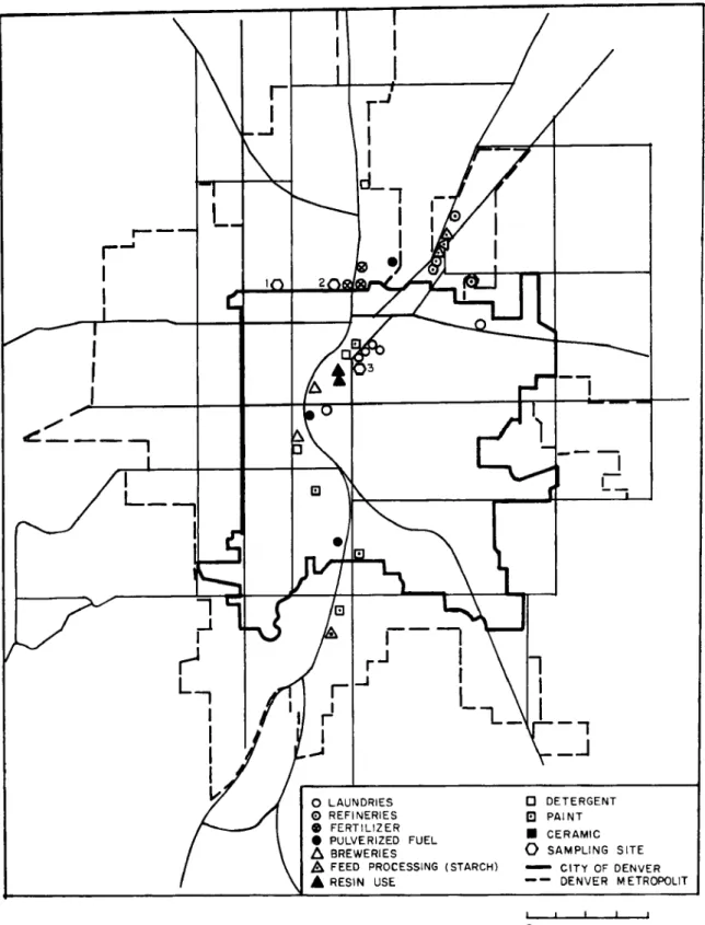
The metropolitan Denver area lies at the foothills east of the Rockies in the South Platte River Valley. The mountain peaks rise to about 8, 000 feet above sea level to the west and to 6, 000 to 7. 000 feet to the southwest. The South Platte River flows from the south-west to the northeast through the heart of Denver which has an average altitude of about 5,250 feet. In Fig. 5 the approximate limits of the populated area and the contours of the terrain are given. Irregularities in the surface due to the different shapes and heights of buildings are not pronounced except in the downtown area. In general, the heights of buildings are between 20 to 30 feet. Some scattered high buildings can be found in other parts of the urban area, but it is supposed that their influence on the general flow patterns is limited to their near
vicinity. It is estimated that pronounced irregularities due to
build-ings, which may affect natural conditions of flow, occupy less than one-tenth of the metropolitan area. Thus. it turns out that the city's topographical influence on the wind regime is not great. The thermal regime of the metropolitan area is not significant. as will be seen in the following paragraphs.
The meteorological network installed for the purpose of moni-toring air pollution occurrences consisted of 17 principal stations at which wind direction and wind speed were recorded and. in most cases. air temperature. These observations of winds were supplemented by data from additional stations operated by the U. S. Weather Bureau at Stapleton Airport. by the U. S. Air Force at Lowry Air Force Base. etc. The number of additional stations varied from seven to three on days with air pollution. The location of all stations is given in Table I
-16-vanes were selected in accordance with recommendations from pre-liminary work (Riehl and Crow. 1962) in order to provide the most representative data.
The air sampling network utilized 22 Paper Tape Air Samplers (Mo. 23000. manufactured by Gelman Ins. Co .• Ann Arbor), The locations of air samplers. as well as of the temperature and wind units. are given in Fig. 5. This network was designed to determine the general level of pollution over the whole city and to evaluate the distribution of pollution within the city for different weather situa.tions.
The level of air pollution is expressed by a "coefficient of
haze". or soiling index. COHo This unit was obtained by relative
measurements of the intensities of light transmitted through clean paper. I • and through soiled paper. 1. Hence. by definition
o
1 COH unit = 100 x optical density (OD)
I
o
where OD = log -1-' The value of COH depends on the volume of air
drawn through the filter paper. If V is the quantity of air sampled in
units of 1000's of linear feet. it follows that:
= flow (ft3/min) x sampling time (min)
V 2
1000 x area of spot (ft )
In addition. the value of COH is normalized for V. thus:
COH
=
OD x 100V
Adjectival ratings were used to determine the level of air pollution in accordance with the basic extensive measurements of smoke concentration prepared by the New Jersey State Department of Hea.lth (1958).
Smoke Concentration COH 0.0-0.9 1.0-1.9 2.0-2.9 3.0-3.9 > 4.0 Adjectival Rating light moderate heavy very heavy extremely heavy
The sampling period was two hours at all stations. On some days with air pollution, supplementary observations were made by ground and aerial photography and by helicopter and wiresonde equip-ment taking temperature soundings, the results of which will be dis-cussed in later sections. The RAOB reports from the U. S. Weather Bureau Station at Stapleton Airport were also used for every day with air pollution.
-18-CHAPTER III
METHODOLOGY Selection of Air Pollution Days
From COH observations, two-hourly maps of contamination were analyzed. The isolines of equal pollution were drawn for every
o.
2 COH. Two examples of COH charts are given in Figs. 6 and 7.However, due to instrumental and operational difficulties, which are to be expected in a field experiment of such scope, it was not possible to obtain continuous measurements of COH at all stations during the two winter seasons. For that reason, the number of stations with usable measurements varied for the several observational times. For example, during 126 selected two-hourly episodes in the 1965-1966 winter season. the number of observations available from all stations was 2,033 instead of the maximum possible 2,268.
The criterion set-up for the selection of days with significant
air pollution was rather subjective. It was partly based on the
adjec-tival rating mentioned previously. Here the difficulty lies in the variability of pollution in time and space so that at some places the contamination may be high while at other places it may be negligible. Nonetheless. the air pollution problem over the Denver city area has to be considered regardless of the small COH values observed at stations in some parts of the city at a given time when pollution is Significant elsewhere. Thus, in order to take into account the COH values over the whole area as well as those at any particular sampling place, a "compromise" criterion was established: Air pollution is
present if the contamination at least at one station is equal to. or
greater than. 1 COH and if the contamination at 50% or more of the remaining stations is greater than O. 5 COH.
It should be of interest to compare COH values for Denver and
22
-measured during the air pollution days at the Adams City Health Center. Denver. during the 1964-1965 winter season with other cities. Averages for the other cities were obtained from daily measurements. not just from measurements during days with significant air pollution.
A basic difficulty in the comparison of COH data between one city and another is the assumption that the optical density of particles deposited on filter paper involves a linear relation to the volume of air filtered with constant area of deposit. Furthermore. the particulates suspended in an urban atmosphere are not of uniform size and the albedo of the deposit strongly depends on the size distri-bution of particulates (Katz et al.. 1958). Sanderson and Katz (1963) concluded that "the simple linear relation between absorbance of smoke stain and the volume of air sampled. although often used. has limited value for comparison purposes". They suggested a standardi-zation of the sampling time. air flow. and area of spot since only under such conditions a comparison between the measurements at different cities would be possible.
On the basis of established critera. 32 days were selected for study of the Denver air pollution (Table II). The total duration of air pollution periods during the two winter seasons was 478 hours.
The Wind Field
The two-hourly mean wind was calculated from the five-minute average values. Examples of the wind record$. wind speed and direc-tion. are given in Fig. 9. Maps of the tWO-hourly mean streamlines and isotachs were constructed from the wind values. applying a kine-matical method (Petterssen. 1956). The wind velocity field is a vector field. given by wind direction and speed at every point in the space
con-sidered. If wind measurements are performed at several points.
direction and speed of wind over an area. Evidently, the denser the observational network. the greater the accuracy in the construction of streamlines and isotachs, provided that "noise" produced by tur-bulence and instrument errors does not disturb the two-hourly mean values.
A streamline is defined as a line which at a given time is everywhere tangent to the wind vector. Thus, the equation of the streamline. written vectorially. is as follows:
or in the Cartesian coordinates;
dx: dy: dz = u: v: w
(1)
(2)
where dr\s a line element of the streamline; dx. dy, dz are its
com-ponents in x, y, and z directions, respectively; and
V
is the velocitywith components u, v. and w.
In our case, the horizontal component of velocity,
V
h was
measured. Then. the streamlines were constructed in such a way
that at every observational point, Eqn. (1) was fulfilled.
The isotachs are by definition the lines of equal wind speed regardless of the direction of the wind. They can be readily analyzed from wind observation.
The two-hourly mean winds were obtained from wind records between two even hours. Thus. the streamline and isotach maps are valid for the middle. uneven hours. Examples of the wind field are given in Figs. 10 and 11.
The Calculation of Horizontal Trajectories
A trajectory is defined as the path of an air parcel. satisfying the condition that the wind vector must be tangent to the trajectory at every moment of time. Since the streamlines at a given time are everywhere tangent to the wind vector too, the trajectories have to
-28-be tangent to the streamlines at the observation time for which the streamline pattern is analyzed. A coincidence between the stream-lines and trajectories can occur only when the wind field remains
stationary.
For the construction of horizontal trajectories~ successive
two-hourly maps of the horizontal wind field were used. A schematic representation of the method for trajectory calculation is given in Fig. 12. From above definitions of the trajectory and streamline. the resulting path of an air parcel. AB:' has to be tangent to the
streamline at time t - ~t. and as time proceeds, must become
tan-o
gent to the streamline at time t ; i. e., the air parcel should describe
o a curve between B" and A.
In our case, "horizontal trajectory" means a trajectory which is parallel to the terrain; it is actually a "quasi" horizontal trajectory.
if one allows for terrain slope. However~ for the sake of simplicity.
it will be called "trajectory".
The Change of Contamination Along a Trajectory
The total change of COH along a trajectory may be obtained from
COH charts at times t and t -.6.t as the difference in pollution between
o 0
the ending and starting pOints (A and B"). This difference may be plotted in the middle of the trajectory if one assumes a linear change of the contamination of the air parcel with time along its trajectory.
This total COH change is equal to the local change during the time interval .6.t. plus the advection term. or
dC
=
aC+
V .
'VC+
w aCdt at h az ( 3)
where
~~
is the total change in COH,~~
is the local change in COH,and
V
-30-vector and \l = _0 -
T
+ _0 -
T
expresses the horizontal gradientoX
oy
oC
operator. The third term on the right side of Eqn. (3), w - - ,
oz
allows far the possibility that an air parcel may experience a vertical displacement during its path between B" and A; this term is referred to as vertical advection; its value will be estimated in the following chapter.
Estimate of Vertical Velocities
In order to obtain an estimate of the vertical velocity field, the most straightforward method is a kinematical one. From wind observations. streamline and isotach charts can be constructed and wind velocity and direction can be determined at any point, though grid points with constant distance are used (Petterssen. 1956). At each grid point. the wind is divided into u and v components. Then the divergence may be obtained as a difference in u and in v at two
successive grid points. When the divergence is computed. the ver-tical velocity can be obtained with the help of the continuity equation, assuming a constant density, or
z
w
= -
J
di vV
h dz o
where
V
h is the horizontal wind vector and z is the height.
(4)
The calculation of w from Eqn. (4) requires high accuracy in the wind observations. A small error in measuring wind direction
and speed will produce a significant error in the divergence. If one
wants to determine the divergence with an accuracy of 10%. the wind
has to be measured within
11/0.
Clearly. such precise windmeasure-ments are not possible with the present standard equipment at a weather station (Thomson. 1961). Therefore, the application of Eqn. (4) in synoptic analysis is limited.
In our case, the error in the divergence was reduced due to the high density of the observation stations and by use of two-hourly mean winds.
The studied area is 180 square miles with 17 principal wind recording stations, a density of approximately one station per ten square miles. This station density is at least 250 times greater than that of the standard meteorological network. In determining this station density, the auxiliary stations were not included because their number varied from time to time. However, data from the U. S. Weather Bureau Station at Stapleton Airport and from Lowry Air Force Base were available at all times during the 1964-1965
and 1965-1966 winter seasons. If these two stations are included,
the density of the observational network further increases and pro-vides for an even higher accuracy in the analysis of the wind fields and in the divergence calculations.
It was mentioned previously that the two-hourly mean wind
was calculated from the five-minute average value. It is assumed
that use of the five-minute period will provide a fairly good estimate of the average wind speed and direction. Examples of wind records from two stations are shown in Fig. 9. At low wind speed, which is common over the Denver city area on days with air pollution, it was possible to determine the five-minute average wind without difficulty. The average values of the two-hourly u and v components (Table III) were small at both sites (Kunsmiller Junior High School and Adams County Health Center), ranging from almost zero to 2. 8 miles/hour
or 0 -1. 4 meters/ sec (roughly 1 meter/ sec = 2 miles/hour). It turns
out that the largest difference in u or v components between adjacent
grid points is
±.
2-3 meters/ sec. Thus .. the divergence has an order-4 -1
-32-where
~x
=~y
= 3 miles'" 5. 5· 103 meters(~x
and~y
are grid dis-tances). By integration of Eqn. (4) from z :::a
to z ::: 10 (the average height above ground of the wind vane), and by taking into account- -4 -1
w :::
a
at z :::a
and that div V h ... 10 sec ,one obtains the order of magnitude of the vertical component of velocity, or-3
w ... 10 meters/ sec .
The five-minute average values may fluctuate around two-hourly means in a wide range. In this case, the two-two-hourly mean wind will have a large probable error, r. The latter can be calcu-lated by the following formula (Panofsky and Brier, 1958):
( 5)
where u. are the five-minute averages from which U, the two-hourly 1
mean is calculated and n is the sample size, in this case 24. The same formula is valid for the v-component.
The probable error, r, is valid for a Gaussian distribution which can be accepted as a fairly good approximation for the wind variations (Pasquill, 1962). The calculation of r for the wind records
shown in Fig. 9 is given in Table IV. For low wind speeds « 1/2 mps),
the probable error in the two-hourly mean can be more than twice as great as the error in the mean wind itself for the u-component and 30 times as great as the error in the mean wind for the v-component since
the latter usually is much weaker than the former. It turns out that the
mean itself does not exceed 1 meter/ sec even with a large probable error in the two-hourly mean wind. At higher values for the two-hourly mean (3 miles/hour), the highest value for the probable error is
approximately 50% of the mean itself so that the true mean lies
between 4. 5 and 1. 5 miles/hour (Table IV, Kunsmiller Junior High
differences in the u or v component do not exceed 5 meters/ sec. Thus, the divergence and w may have maximum values of the order
-3 -2
of 10 and 10 ,respectively. However, the value for w was never
higher than 3· 10-3 meters at any point during the 1964-1965 winter
season. This corresponds to a vertical displacement of the air particles of 20 meters in two hours. An example of this vertical displacement is given in Fig. 13 on the 3 February 1965, 02-04 MST. As can be seen, this displacement does not exceed 13 meters for two hours.
In proof of the normal distribution for the five-minute averages, the following formula is applied (Conrad, 1950):
-I+-
71"L
(u. - u) 1= - X =
-2 n ( 6)
The result given in Table IV shows an absolute difference in the standard deviation calculated from data (Table III) and with the
help of formula (6). Only in one case the difference between right and
left side of Eqn. (6) is as large as . 21. This is an effect of the extremely large number of five-minute averages with zero values. In this case the two-hourly mean depends on the extremes.
Estimate of the Horizontal and Vertical Advection
The order of magnitude of the horizontal and vertical
advec-tion can be estimated from the values of
V
h • w, V'C, and oC •
oz
The magnitude of the vertical velocity, w, has been discussed in detail-3
before. It was found to be w ... 10 meters/ sec. Furthermore, it
was shown that the two-hourly mean wind is light; its value varies from between zero and three meters per second, taking into account the probable error. This is a common range of the horizontal wind speed as can be seen from the two examples of the wind field shown in Figs. 10 and 11.
The horizontal and vertical gradients of COH may be estimated from the charts of contamination and from the observations of COH at two different levels. In order to compare the horizontal and vertical gradients of COH. measurements of COH in the vertical and in the horizontal directions had to be performed simultaneously.
The vertical gradient. aC • was calculated from observations az
performed in Denver at Signal Broadcast Production. Inc .• 1601 Arapahoe Street. at an elevation of 324 feet above the ground. and at the CSU Field Office. 23rd and Broadway Streets. at 12 feet above the ground. The horizontal distance between these two observational sites is .7 miles. For this calculation. the period between 10 MST on 8 December to 10 MST on 9 December 1965 was chosen. From the COH chart for the same period. \7C was calculated from grid points three miles apart; however. only those pOints at which the analysis was certain were taken into account (see Fig. 6 for analysis and grid). From 12 charts. 107 values were taken or an average of nine points per chart. In this manner. a better value for \7C over the whole is obtained than could be from two points only. The calcu-lation is given in Table V. and the results are shown in Fig. 14. The difference between two gradients is evident: aC is at least one
az
order of magnitude higher than the corresponding value for \7C at
any time of day even though it never reached 10-1 .
o -3 -4
Consequently. since V ... 10 • w ... 10 • \7C ... 10 • and aC ... 10 -2 the value of the horizontal advection is at least one
az •
order of magnitude higher than the value of the vertical one. or
- -4 aC -5
V . \7C ... 0 (l0 ) w - '" 0 (l0 ).
h • az
For that reason. it is assumed that the horizontal wind is responsible for the transport of polluted air over the city and that. therefore. the third term on the right side of Eqn. (3) can be neglected.
The Errors in the Trajectory Calculations
Regardless of the small value of the vertical velocity cal-culated from the wind field, an air parcel may be affected by the temperature field and the vertical wind profile. For example, high temperatures at low levels of the atmosphere will produce an upward motion of the air parcel due to the difference between the density of the air parcel and that of its environment. The vertical acceleration of the air parcel is proportional to the difference in temperature
between the air parcel and its environment, assuming that the pressure of the air parcel and its environment are the same.
Over Denver, the surface temperature field shows the effect of the well-known phenomenon of "the city heat island". That is, the difference in temperature between the downtown area and the suburbs
o
may reach as much as 10 F. Such a difference can generate vertical motion over the "heat island" which may affect the horizontal tra-jectory.
The Denver RAOB reports show the presen"ce of a strong inver-sion in the lower layer ( ... 1500 feet) of the atmosphere which is in excess of at least twice the horizontal temperature difference. An example of the Denver RAOB report is given in Fig. 15 for 7 December 1965 at 05 MST. The temperature field for this day (Fig. 16) shows "the city
heat island" over the downtown area with a temperature of 46oF. If
the average height of buildings in downtown Denver is assumed to be 100 feet, an air parcel will attain the same temperature as in the free atmosphere at 90 feet above roof level. under the assumption that the temperature of the air parcel decreases with height dry-adiabatieally. This vertical distance is negligible in comparison with the horizontal one which an air parcel traveled during two hours. Furthermore, the
temperature at Kunsmiller Junior High School is 4SoF at the elevation
5,535 feet above m. s. 1. The same temperature in the free atmosphere
Soiling Index
CHAPTER IV ANALYSIS
For the ten sampling sites, which had a large number of observations during the 1964-1965 and 1965 -1966 winter air pollu-tion seasons, the daily course of two-hourly average COH values is given in Fig. 19. The average values are plotted at the mid-point of the sampling period.
In the northern part of the city (the stations: State Game, Fish. and Parks Department. Northridge Lumber Company. Adams City Health Center, Denver Sewage Treatment Plant and Wheatridge Sanitation District). the maximum COH occurs at nine o'clock in the morning and the minimum in the middle of the afternoon. Secondary extremes occur at nine o'clock in the evening (maximum) and in the early morning (minimum).
The daily course of contamination is a function of both the rate of emission and meteorological conditions. The morning peak may be ascribed to increasing business activity at this time of day. The occurrence of the primary minimum in the afternoon. between one o'clock and three o'clock. can be attributed to the warming of the lowest layer of the atmosphere due to solar heating which increases the vertical mixing. The displacement of the maximum to the afternoon at the Signal Broadcast Productions. Inc.. in the downtown area at 324 feet above the ground. may also be related to the increasing of vertical mixing. Such an explanation for the after-noon minimum is suggested by Riehl and Crow (1961). However, another possibility exists: The afternoon minimum may be due to both the warming of the lowest layer of the atmosphere and the pre--vailing wind at this time of the day. The latter may bring cleaner air into the region and in this manner decrease pollution. The
-46-morning peak is generally ascribed to "fumigation"l (Hewson, 1961), which depends on the vertical stability of air (see Fig. 2). However. one would not expect the occurrence of fumigation under inversion con-ditions in the lowest layer of the atmosphere, but rather a "fanning,,2 (Gosline et a1.. 1956).
The two stations in the southern part of the city. Kunsmiller Junior High School and Arapahoe Health Center, show the steady increasing of pollution from the morning to the afternoon with a maximum between three o'clock and seven o'clock, which is most pronouneed at the first station. Thus, these stations show a daiJ.y course opposite to that of the stations in the northern part of the city. The cause for this diurnal change will be explained later.
It is a fairly good assumption that the strength of sources responsible for the contamination of air over the Denver area. was not different in the two winter seasons. Since the daily course of COH has the same characteristics in both air pollution seasons, one may conclude that the same factors are responsible for the similar daily course of contamination in different parts of the city. This will be studied in the following pages.
The charts of mean COH values are given in Figs. 20 and 21. For the majority of the stations, the mean values were obtained from large samples and these means may be accepted as very close to the real level of the average contamination during study days with air pollution. As can be seen, the city area with heaviest pollution lies along the South Platte River Valley.
I The phenomenon referred to as "fumigation" occurs during a transition from smooth to turbulent flow. Generally, it is caused by heating of the lower layer of the atmosphere from the ground.
2"Fanning" is another characteristic shape of plume when an inversion is present. A "fanning plume" has a very small extent in the vertical direction and due to slight shifts in wind direction, the plume meanders downwind in the shallow layer.
The Wind Field
For the two air pollution seasons. the flow patterns over the Denver area may be divided into four major groups:
(0 S-SW winds, downslope motion, drainage wind down the
Platte HiveI' Valley;
(2) N -NE winds, upslope motion, also along the river valley
with some deflection along mountain side s;
(3) A combination of (1) and (2) with a convergence line which
moves over Denver. This type of flow is associated with very light winds or almost calm conditions. It occurs during the turning of
S·-SW to N - NE flow, and vice versa. Its duration is usually from
two to four hours. For the sake of simplicity. this flow will be called N-'S;
(4) SE winds, observed in only 14 cases.
The occurrence of the S-SW type of flow makes up 56C1c O~3
cases) of the whole sample period, while N -NE makes up 27% (C3
cases). Thus, these two flow patterns provide a sufficiently large sample for a study of the motion of pollutants. Clearly, the center of attention should be N-NE and S-SW situations. An attempt was also made to study the N -S type, but the result was not satisfactory due to the very light winds and the calm conditions at the majority of the stations. Uncertainties in the streamlines, as well as in the iso·-tach analyses, are unavoidable under these conditions. Moreover. the position of the convergence line is questionable. The small
number of case s with N - S flow. only 11 % or 27 case s during the
whole sample period, does not permit one to draw any statistically meaningful conclusions. For the same reason. the SE flow has not been considered either.
The analyse,::; show that the downslope (S-SW) flow usually begins between seven oiclock and ten o'clock in the evening and lasts until noon the next day. after which time the flow changes to
-50-N - -50-NE type. This reversal of the wind flow will be studied in the following section.
An example of the two-hourly average streamlines and
isotachs in S-SW flow is shown in Fig. 10. As can be seen. the
influence of topography on the wind field is very well marked. The streamlines strictly follow the shape of the terrain; the small hill in the northeastern part of the Denver metropolitan area. and the tributary valleys on the west and east of the South Platte River (Layden Creek. Turkey Creek. Cherry Creek. etc.) have a well,-defined influence on the direction of flow. As was shown previously. the wind speeds are light over the whole area.
The influence of the terrain on the N-NE (Fig. 11) type of flow is almost the same. Thus. the topographic features around Denver strongly determine the wind direction and speed when the general weather situation is characterized by very light winds aloft and subsidence. The strong inversion may persist for several days during which the wind flow has a direction in the night and morning hours (S-SW) opposite from the one in the afternoon (N-NE). In such weather situations, the movement of a polluted air mass is very slow along the South Platte River Valley. and one may expect that the poIlu'-tion is not transported very far away from the city limits. Gifford (1953). in his study of low-level air trajectories using zero-lift balloons. has shown that under inversion conditions the balloon paths obeyed downslope motion and were closely parallel to the terrain. Neiberger (1961) studied the change of the hydrocarbon and CO con·-centrations along an air parcel trajectory over Los Angeles and found a good agreement between the amounts of cumulative contamination along a trajectory and the observed value measured at the end point of the same trajectory_
reversed to S-SW in the early evening, and this flow lasted until noon of the next day. During certain days, the reversal of flow did not occur as, for example, on the 18, 28, and 29 of December 1965. During these days, the RAOB reports showed increasing wind speeds at 6.000 and 7.000 feet (15 to 20 knots), indicating that the daily wind regime did undergo changes under the influence of the large scale weather pattern which caused a strengthening of the pressure gradient and an increase of the wind. Furthermore. the non-appearance of the daily reversal in the wind flow during these three days was associated with the break in the air pollution episode. Wind speed at the surface increased until eleven o'clock on 18 December 1965 when the wind reached almost 10 mph. The same phenomenon occurred on the morning of 29 December 1965. In both cases, inversions of the temperature existed. Thus, increasing wind speeds at the surface and in the lower layer of the atmosphere are sufficient to alleviate or terminate air pollu-tion situapollu-tions over Denver.
The vertical temperature profiles taken from the RAOB reports showed a presence of the temperature inversion during the night and morning. The strength of the inversion, as well as its depth, varied during the day. Morning lapse rates attained
o
values to -9
elI
00 meters, with the most frequent value of abouto
-5
ellOo
meters. In some cases, the temperature inversion wasbroken in the lowest layer of the atmosphere during the daytime and the lapse rate reached a positive value (see, for example, Fig. 23). When such a situation of a weakening or breaking inver-sion occurred, the air pollution period was not necessarily ended. On occasions even an increase of COR appeared in the southern part of the city in the afternoon, as was the case on 17 December 1965, typical for many other days. In these cases, the wind speeds at the surface as well as at 220 and 550 meters above the ground
-62-were rather small. less than 5 knots. Thus. the breaking or weakening of the inversion was not by itself sufficient to end air pollution over Denver.
It was mentioned earlier that two stations in the southern
part of the city (Kunsmiller Junior High School and Arapahoe Health Center) show. on the average. a steady increase in pollution from
morning to afternoon with the maximum reached at sunset. It is
possible to relate the occurrence of COR extremes in the different parts of the city to the prevailing winds and to the height of the
inversion layer. It can be seen from Fig. 23 that the onset of
N-NE flow is associated with decreasing COR values in the northern-most part of the city (squares 3 and 6). By afternoon, either the depth of the lowest inversion layer increased or the inversion shifted to some height above the ground. In both cases, the pollu-tion layer extended to the height of 200 to 300 meters above the ground. and the occurrence of "fanning" or "fumigation" at the highest elevation above the ground was common (see Fi.g. 2).
Stronger pollution will be found in the areas with higher elevations. In Denver these are the southern parts of the city. Thus, the trans-port of polluted air in N - NE flow during the afternoon and the change of the temperature profile during the daytime were responsible for the occurrence of COH maxima in the late afternoon in the southern section of the city_
In Fig. 24 the mean COR values for the northern and for the southern areas of the city (squares 3 and 6, 14 and 18. respectively) are given with respect to the prevailing flow during different times of the day for December 6 to 10 and December 16 to 18, 1965. As can be seen from this figure. COR mean values during S-SW flow show increases in the northern part of the city and decreases in the southern part. An opposite COR course was associated with N-NE flow. On the basis of Fig. 23, one may safely conclude that the
-68-one cannot conclude that the city area is the main source of air pollu-tion because the local change of COH. a; , is included in the total
dC
a
one,
ill.
From Eqn. (3), after neglecting the vertical advection.it follow s that
dC _ aC __
--V·'VC
dt at (7)
b b d f dC" d b "
The local change has to e su tracte rom
ill
m or er to 0 ta.m ah Orlzon a a vec Ion. " t 1 d t" A map 0 f
at
aC" IS gIven In " "F" 19. 27"t ; 1 wasobtained by subtracting the corresponding maps of COHo The final
step is a subtraction of two fields,
~;
-~;
• (Figs. 26 and'~7).
and the result is shown in Fig. 28. As can be seen. the area with negative advection lies along the South Platte River in the northeast-ern part of the metropolitan area. This means that the local change. or the production of the pollutant in this area. is stronger than its transport by flow into this area. Such a conclusion is drawn on the basis of only one episode with S-SW flow. To find whether this con-clusion holds on the average, all S-SW situations have to be studied. This will be discussed in the following pages.
During the N-NE flow~ the trajectories of the air parcels show
an opposite transport of pollution (Fig. 29). Corresponding maps of the local and total COH change and advection are given in Figs. 30. 31. and 32. The difference in the advection between S-SW and N-NE wind patterns is evident (compare Figs. 28 and 32). During N-NE flow the advection is positive in the northern part of the city, but in the
southwestern and southeastern parts, it is negative. It will be seen
later that such a distribution of advection during N-NE flow is valid on the average and not only for this specific case. For the moment it shall be stressed that a pronounced difference exists in the va.lues of advection over the city during these two types of wind flow.
In the case when the flow changes from S-SW to N-NE. the resulting wind patterns and their corresponding trajectories show
pronounced changes in the advection over different parts of the city. Examples are given in Figs. 33, 34, and 35 for 8 December 1965. At 09 MST the wind field (Fig. 33) had a pronounced S-SW direction, and its flow was very similar to that in the previous example (Fig. 10). The trajectories strictly followed streamlines
indicating a stationary wind field, and an advection map
(V.
\7C )showed in general the same distribution of positive and negative regions, as was shown in the above mentioned case. At 11 MST the majority of stations experienced a reversal of wind direction from S·-SW to N -·NE (Fig. 34). The corresponding trajectories (obtained from two successive wind fields at 09 and at 11 MST) show that the air parcels turned over the city from the north to the south. Net advection was rather weak over the entire city area because the air parcels reversed their track. Complete reversal of the wind occurred at 13 MST at all stations except two in the southernmost part of the area. At this hour, the paths of the air parcels were oriented to the south, and the corresponding advec-tion was opposite to that at 09 MST (compare Fig. 35 to Fig. 33).
It was mentioned earlier that an increase in wind speed is sufficient to end severe air pollution over Denver. When such an increase occurs and it is followed by the breaking up of the inversion, the polluted air disperses very rapidly in both the horizontal and
vertical directions. An example of such dispersal of air pollution
over Denver is given for 10 December 1965. On the morning of this day (09 MST), the wind was light and the COH values at the majority of stations were higher than 1 (Fig. 36). The trajec-tories were very similar to those given in the previous examples with N-NE flow. However, from that time until noon the surface wind increased. and at 13 MST on that same day, it reached 6 mph at one station in the northern part of the city (Fig. 37). Now the COH values were less than one except for two stations in the south-eastern part of the city. On this morning the inversion had been
o
230 meters thick with 'Y
=
-2. 6 C, as may be seen from Fig. 23.Before 11 MST, warming had destroyed the inversion and it had caused free mixing of the air in the vertical. This mixing, together with an increase in surface wind, exported the polluted mass from the city. By noon, the two-hour air parcel trajec-tories over the city (Fig. 37) had become rather long, indicating the fast movement of air and the dispersion of pollution.
-82-CHAPTER V SUMMARY OF RESULTS
In order to evaluate the average advection during the S-SW and N-NE flow patterns, the whole metropolitan area was divided
into equal squares with sides of three miles each (Fig. 22).
Employ-ing a weightEmploy-ing method; the values of advection were computed. The average values of advection for all S-SW and all N-NE flows
were plotted in the center of the corresponding squares. It should
be emphasized that the minus sign indicates the region of sources, and the positive sign indicates the transport of polluted air. The average maps show which factor- -the advection or the sources--contributed more to the level of pollution in the various parts of the city.
The average of horizontal COH advection during downslope S-SW flow is given in Fig. 38. The maximum of positive advection is found in the southwestern part of the area as it was in the pre-vious examples for S-SW flow (square numbers 13 and 14). In the northeastern part of the city during S-SW flow, one would expect the highest rate of advection since an air parcel passing over the city becomes more and more contaminated from numerous sources located along its route. In spite of this fact; contamination from the local sources on the average exceeds the effect of advection by more than a factor of 10. The frequencies of advected COH for all squares during S-SW flow are given in Table VI.
The values in square numbers 7 and 8 are rather small indi-cating that the contributions of advection and of local sources to the pollution in this part of the city are the same. In other city regions the average advection in S-SW flow exceeds the influence of local sources by at least five times (Table VI).
-84-During N - NE flow a distribution of the average advection occurs over the city opposite to the one observed during a S-SW situation (Fig. 39), In the northeastern part of the metropolitan area, the advection on the average contributed to the contamina-tion more than the local sources do (Table VII. square numbers 1 to 4 and 6 to 8). In the southern part of the city, the influence of the local sources is a little greater on the level of pollution than that of advection. Such values of advection in these two areas are in agreement with the previous examples for N - NE flow. In
other squares the average advection is small. It indicates the
high rate of alternation between the transport of pollution from adjacent areas and its introduction from local sources.
Such distributions of the average advection during S-SW and N - NE wind patterns require explanations. In the northeastern part of the metropolitan area, along the South Platte River. the alterna-tion of positive and negative advecalterna-tion occurs in connecalterna-tion with the change of flow patterns. Positive values of advection occur during N - NE flow and may be ascribed to the insufficient dilution of polluted air outside the limits of the metropolitan area or to the additional increment of pollution taking place outside the area. However. the N - NE flow prevails during the afternoon when the minimum of COH occurs at stations located in the same region (see Fig. 19). Thus. a cleaner air is brought into the area and causes a decrease of pollution. In spite of such a coincidence. the transport of the polluted matter outward is greater than the local change of COH during the same time as can be seen from Table VIII. This implies that the emission rate of polluted matter into the atmosphere in the northeastern part of the metropolitan area is smaller during the afternoon.
In the southwestern part of the city. the daily maximum of COH occurs during the afternoon when the N - NE flow is prevailing
-86-(see Fig. 19). At the same time, the average value of the advection has a negative sign; i. e .• the emission rate of pollutants within the
area exceeds the transport of pollutants into it, although the differ-ence between the two is small. Thus, the occurrdiffer-ence of the daily maximum during the afternoon may be attributed to the sources within the area as well as to the advection of pollutants from the adjacent regions.
CHAPTER VI CONCLUSIONS
The horizontal trajectories of the air parcels provide useful information of the movement of the polluted mass over the metro-politan area. A local circulation pattern with a pronounced daily variation exists over Denver during days with air pollution and the influence of the topography on the wind field is dominant. The dis-persion of pollutants is reduced due to the light winds and the temperature inversion in the lower layer of the atmosphere.
The daily course of COH has different characteristics in the northern and in the southern parts of the metropolitan area. It depends on the business activity and on the circulation pattern during different times of the day.
The polluted mass of the air follow s the horizontal wind
field, and it moves along the South Platte River Valley. An air
parcel becomes more and more polluted during its progress over the city, but the main increase to its pollution is obtained i.n the northeastern part of the metropolitan area.
ACKNOWLEDGEMENTS
The author wishes to acknowledge the guidance and sugges-tions by Professor Herbert Riehl and Professor Elmar Rei.ter. He also benefited from discussions wi.th Dr. William Marlatt.
The author wishes to express his appreciation to Mrs. Kosara Markovic and Miss Brana Ckonjevic who drafted the diagrams and to Mrs. Sandra Olson who typed the manuscript.
Valuable computational assistance was obtained through the computer facility at the National Center for Atmospheric Research in Boulder.
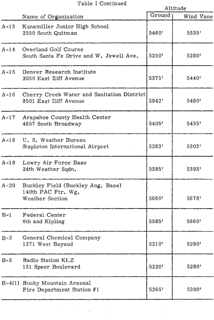
A-1 A-2 A-3 A-4 A-5 A-6 A-7 A-8 A-9 A-10 A-ll A-12 -88-TABLE I LOCATION OF STATION Name of Organization Northridge Lumber Co.
7900 North Federal Boulevard
Adams City Health Center 4301 East 72nd Avenue
Wheatridge Sanitation District 4900 Marshall
Denver Sewage Treatment Plant 52nd and Downing
Yellow Cab Company 3455 Ringsby Court Yellow Cab Company 3455 Ringsby Court
Barteldes Seed Company 3770 East 40th Avenue Jefferson High School 2305 Pierce Street
Denver School Administration Building 414 14th Street
State Public Health 4210 East 11th Avenue
Hested Store Company
185 South Sheridan Boulevard Byers Junior High School 150 South Pearl
Altitude
Ground Wind Vane
5380' 5400' 5110' 5135' 5300' 5315' 5140' 5215' 5160' 5400' 5300' 5160' 5200' 5270' 5300'
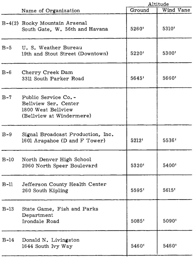
-5350' 5380' 5225' 5300' 5310' 5390' 5400' 5450' 5285' 5315'Table I Continued
Altitude
Name of Organization Group.d Wind Vane
A-13 Kunsmiller Junior High School
2250 South Quitman 5460' 5535'
A-14 Overland Golf Course
South Santa Fe Drive and W. Jewell Ave. 5250' 5280'
A-15 Denver Research Institute
2050 East iliff Avenue 5375' 5440'
A-16 Cherry Creek Water and Sanitation District
8501 East Iliff Avenue 5942' 5480'
A-17 Arapahoe County Health Center
4857 South Broadway 5405' 5435'
A-18 U. S. Weather Bureau
Stapleton International Airport 5283' 5303'
A-19 Lowry Air Force Base
24th Weather Sqdn. 5385' 5393'
A-20 Buckley Field (Buckley Ang. Base) 140th PAC Ftr. Wg.
Weather Section 5660' 5678'
B-1 Federal Center
6th and Kipling 5585' 5660'
B-2 General Chemical Company
1271 West Bayaud 5210' 5280'
B-3 Radio Station KLZ
131 Speer Boulevard 5220' 5280'
B-4(1 ) Rocky Mountain Arsenal
90
-Table I Continued
Altitude
Name of Organization Ground Wind Vane
B-4(2) Rocky Mountain Arsenal
South Gate, W. 56th and Havana 5260' 5310'
B-5 U. S. Weather Bureau
19th and Stout Street (Downtown) 5220' 5300'
B-6 Cherry Creek Dam
3311 South Parker Road 5645' 5660'
B-7 Public Service Co.
-Bellview Sere Center 1800 West Bellview
(Bellview at Windermere)
B-9 Signal Broadcast Production. Inc.
1601 Arapahoe (D and F Tower) 5212' 55:36'
B-IO North Denver High School
2960 North Speer Boulevard 5320' 5400'
B-ll Jefferson County Health Center
260 South Kipling 5595' 5615'
B-13 State Game, Fish and Parks
Department
Irondale Road 5085' 5090'
B-14 Donald N. Livingston
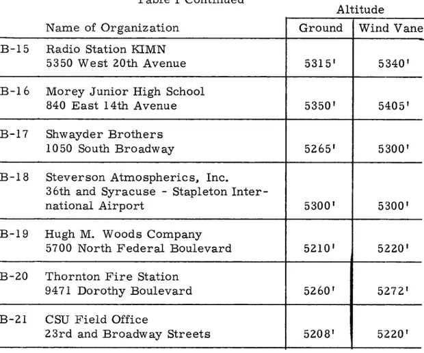
Table I Continued
Altitude
Name of Organization Ground Wind Vane
B-15 Radio Station KIMN
5350 West 20th Avenue 5315' 5340'
B-16 Morey Junior High School
840 East 14th Avenue 5350' 5405'
B-17 Shwayder Brothers
1050 South Broadway 5265' 5300'
B-18 Steverson Atmospherics. Inc.
36th and Syracuse - Stapleton
Inter-national Airport 5300' 5300'
B-19 Hugh M. Woods Company
5700 North Federal Boulevard 5210' 5220'
B-20 Thornton Fire Station
9471 Dorothy Boulevard 5260' 5272'
B-21 CSU Field Office
-92-TABLE II
Days With Air Pollution in Denver 1964-1965 January 20-22 February 1-4 February 8-9 February 16-19 March 25-26 Winter 1965-1966 December 6-10 December 16-18 December 27 -29 January 5-6 January 12-13 February 6-7
*
TABLE IVThe Probable Error in u and V and Check for a Gaussian Distribution of the Five-Minute
Average Wind (Sampling Time 2 Hours) 3 February 1965 Time +r +r Station (hours) u - u v -v
-
-Adams City 00-02 .65 .60 .58 .65 Health Center 02-04 .25 .43 .01 .31 Kunsmiller Jr. 00-02 .55 1. 33 2.82 1. 57 High School 02-04 1.68 1. 34 2.92 .94*
Data From Table III.**
Given in absolute value (see formula 6 on page 33Check Difference** .00 .05 .14 .02 .01 .03 .03 .21
).
WITH DENVER AIR POLLUTION WIND DATA
by
William D. Ehrman
ABSTRACT
Machine procedures used in this study are explained in detail. including possible applications of these developed tech-niques to real time data acquisition and presentation installa-tions.