Analyzing Potential Improvements to a Semi-Analytical CO
2Leakage
Algorithm
Brent Cody1, Ana González-Nicolás, Domenico Baù
Department of Civil and Environmental Engineering, Colorado State University
Abstract. A long history of using of fossil fuels has resulted in increased atmospheric CO2 concentrations. This anthropogenic process has influenced global climate change. One possible
way to retard this increasing atmospheric concentration is to geologically sequester CO2 emissions.
Successfully implementation of this technology requires a full understand of associated risks and detailed resource optimization. It is important to choose the appropriate level of complexity when selecting the type of simulation model to apply to this problem. Many risk assessment and
optimization tools require large numbers of realizations. In most cases, using a full scale numerical
CO2 leakage model for this process becomes computationally prohibitive. Therefore, faster CO2
leakage estimations are needed. An excellent semi-analytical multi-phase CO2 leakage algorithm
has been developed by Celia et al. (2011). In the following work, three possible accuracy
improvements to this algorithm are proposed and explored. Differences between leakage rates and pressure distributions are compared between existing and modified methods. Improvement
suggestions are then made from these observations.
Introduction
Preliminary stages of geological storage (GS) site selection, optimization, and sensitivity analysis require large numbers of model simulations. It is often beneficial to use faster, though less accurate, leakage estimation models for ‘coarse’ scale project development. After narrowing down the set of possible solutions, more sophisticated, although slower, numerical models should be used for detailed project development.
A semi-analytical algorithm, developed by Celia et. al. (2011) and Nordbotten et.
al. (2009), estimates both brine and CO2 flux through permeable caprock locations caused
by GS. Originally conceptualized as segments of abandoned wells, permeable caprock locations represent cylindrical portions of the aquitard layers having permeability values greater than or equal to zero. Referred to as ‘leaky wells’, these are the only pathways for fluid flux between aquifer layers.. Users of this model are able to specify the number and spatial location of injection wells (M), leaky wells (N), and aquifer/aquitard layers (L).
The domain is structured as a horizontal stack of aquifer/aquitard layers perforated by injection and leaky wells. Aquifers are assumed to be horizontally level, homogenous, and isotropic. Aquitards are impermeable, except where perforated by leaky wells. Injection wells are able to inject into any layer.
1 Groundwater Hydrology Division Civil Engineering Department Colorado State University Fort Collins, CO 80523-1372 e-mail: codybm@engr.colostate.edu
Figure 1. Domain Schematic
Initially, fluid is not flowing through any of the leaky wells because the entire domain is assumed to be saturated with brine at hydrostatic pressure. At the start of fluid injection the pressure throughout the domain begins to change resulting in fluid flux through leaky wells. It is therefore very important to understand aquifer fluid pressure
responses regarding changes in CO2 and brine storage volumes. Celia et. al. (2011)
presents the pressure distribution in a confined aquifer for a single well injecting CO2 as
∆𝑝! 𝜒 − 𝐹 ℎ! = 0, 𝜒 ≥ 𝜓 −2Γ1 ln 𝜓𝜒 + ∆𝑝! 𝜓 , 𝜓 > 𝜒 ≥ 2𝜆 1 Γ− 𝜒 Γ 2𝜆+ ∆𝑝 ! 2𝜆 , 2𝜆 > 𝜒 ≥2 𝜆 − 1 2𝜆Γln 𝜒𝜆 2 + ∆𝑝! 2 𝜆 − 𝐹 ℎ! , 2 𝜆 > 𝜒 (1) where 𝜒 =2𝜋𝐻𝜑 1 − 𝑆!!"# 𝑟! 𝑄!"##𝑡 (2) Γ =2𝜋 𝜌!− 𝜌! 𝑔𝑘𝐻! 𝜇!𝑄!"#! (3) 𝜓 =4.5𝜋𝐻𝜑𝑘 1 − 𝑆! !"# 𝑟! 𝜇!𝑐!""𝑄!"## (4)
∆𝑝! = 𝑝 − 𝑝! 𝜌!− 𝜌! 𝑔𝐻 (5) ℎ! =ℎ(𝜒) 𝐻 = 1 𝜆 − 1 2𝜆 𝜒 − 1 (6) 𝐹(ℎ′) = −𝜆 𝜆 − 1 h′ − 𝑙𝑛 𝜆 − 1 ℎ′ + 1 𝜆 − 1 (7)
In (1-7), subscripts b and c denote brine and CO2, respectively, λ refers to total
aquifer mobility. B, H, and h are aquitard, aquifer, and CO2 plume thicknesses,
respectively. 𝑆!!"# is the residual saturation of the brine, t is injection duration, k is permeability, 𝑐!"" is the effective compressibility of the aquifer, g is gravitational acceleration, µ is dynamic viscosity, ϕ is porosity, r is radial distance, ρ is fluid density, and 𝑄!"## is the total volumetric well flux. F(h’) is an offset term resulting from solving the ordinary differential pressure equation (17) in Nordbotten and Celia (2006).
The semi-analytical algorithm uses (1) to determine the pressure distribution throughout the aquifer then applies the multiphase version of Darcy’s law to determine leaky well flow rates.
𝑄!,!"##,! = 𝜋𝑟!"!"##,!! 𝑘!,!𝑘!"##,!
𝜇!𝐵! 𝑝!"##,!!!− 𝜌!𝑔𝐵!− 𝑔𝜌!𝐻!!! − 𝑝!"##,!
(8)
In (8) kr is relative conductivity and α denotes phase type (either c for CO2 or b for brine).
Unlike the Theis Equation, (1) is both non-linear and discontinuous. Also, unlike
single phase flow, CO2 plume locations and thicknesses must be known when determining
fluid saturations and relative permeabilities found in leaky well pathways.
These problems are overcome by linearizing the pressure equation using Green’s functions and applying time-stepping to approximate the changing pressure distribution,
CO2 plume locations and thicknesses, and leaky well fluxes over the injection duration.
For each time-step, the following linear equation is written for each leaky well at the bottom of each aquifer.
𝑝!,! = 𝑝!"#,!+ 𝐺!,!,!"##𝑄!"##,! ! !"##!! + 𝐺!,!,!"## 𝑄!"##,! − 𝑄!"!!,!!! !!! !"##!!!! + 𝐹(ℎ!"#! ) (9)
In (9) p is the fluid pressure at the bottom of the aquifer, w denotes the well at which pressure is being solved, l denotes the aquifer layer, well denotes the well flux adding or subtracting pressure at well w. Also,
𝐺!,!,!"## = 𝜕𝑝!,!
𝜕𝑄!"##,! (10)
Nordbotten et. al. (2009) describes these Green’s functions as representations of “the sensitivity of the pressure field for a given source or sink”. They are found by
calculating the partial derivative of (1) with respect to 𝑄!"##. For each time-step, Green’s
functions are evaluated using start of time-step flow rates. This results in 𝐺!,!,!"## being a constant value for each time-step.
Figure 2. Pressure unknowns for this domain are located at the red circles Substituting (8) into (9) yields the following,
𝑝!,! = 𝑝!"#,!+ 𝐺!,!,!"##𝑄!"##,! ! !"##!! + 𝐺!,!,!"## 𝜋𝑟!"!"##,!! 𝑘 !"##,! 𝑘!,!"",!"##,! 𝜇!""𝐵! 𝑝!"##,!!!− 𝜌!𝑔𝐵! !!! !"##!!!! − 𝑔𝐻!!!(𝜌!− 𝜌!ℎ!,!!!! + 𝜌 !ℎ!,!!!! ) − 𝑝!"##,! − 𝜋𝑟!"!"##,!!!! 𝑘 !"##,!!! 𝑘!,!"",!"##,!!! 𝜇!"!𝐵!!! 𝑝!"##,! − 𝜌!𝑔𝐵!!! − 𝑔𝐻! 𝜌!− 𝜌!ℎ!,!! + 𝜌 !ℎ!,!! − 𝑝!"##,!!! + 𝐹(ℎ!"#! ) (11)
where the subscript eff denotes ‘effective’. Effective phase dependent parameters are
needed because 𝑄!"## may be composed of both CO2 and brine. It is now possible to
isolate the unknown pressure terms 𝑝!,!, 𝑝!"##,!!!, 𝑝!"##,!, and 𝑝!"##,!!!. 𝑝!,! + −𝐺!,!,!"##𝜋𝑟!"!"##,!! 𝑘 !"##,! 𝑘!,!"",!"##,! 𝜇!""𝐵! 𝑝!"##,!!! !!! !"##!!!! + 𝐺!,!,!"##𝜋𝑟!"!"##,!! 𝑘!"##,! 𝑘!,!"",!"##,! 𝜇!""𝐵! + 𝐺!,!,!"##𝜋𝑟!"!"##,!!!! 𝑘 !"##,!!! 𝑘!,!"",!"##,!!! 𝜇!""𝐵!!! 𝑝!"##,! + −𝐺!,!,!"##𝜋𝑟!"!"##,!!!! 𝑘 !"##,!!! 𝑘!,!"",!"##,!!! 𝜇!""𝐵!!! 𝑝!"##,!!! = 𝑝!"#,!+ 𝐺!,!,!"##𝑄!"##,! ! !"#!!! + 𝐺!,!,!"## 𝜋𝑟!"!"##,!! 𝑘!"##,! 𝑘!,!"",!"##,! 𝜇!""𝐵! −𝜌!𝑔𝐵! !!! !"##!!!! − 𝑔𝐻!!!(𝜌!− 𝜌!ℎ!,!!!! + 𝜌 !ℎ!,!!!! ) − 𝜋𝑟!"!"##,!!!! 𝑘 !"##,!!! 𝑘!,!"",!"##,!!! 𝜇!""𝐵!!! −𝜌!𝑔𝐵!!! − 𝑔𝐻! 𝜌!− 𝜌!ℎ!,!! + 𝜌 !ℎ!,!! + 𝐹(ℎ!"#! ) (12) (12) can be written as 𝑝!,!+ 𝐴!,!,!"##𝑝!"##,!!!+ 𝐵!,!,!"##𝑝!"##,!+𝐶!,!,!"##𝑝!"##,!!! !!! !"!!!!!! = 𝐷!,! (13)
where A, B, C, and D are constants for the current time-step. The set of linear equations in matrix form for a domain having 3 aquifer/aquitard layers and 2 leaky wells would be written as 𝐵!,!,!+ 1 𝐵!,!,! 𝐶!,!,! 𝐶!,!,! 0 0 𝐵!,!,! 𝐵!,!,!+ 1 𝐶!,!,! 𝐶!,!,! 0 0 𝐴!,!,! 𝐴!,!,! 𝐵!,!,! + 1 𝐵!,!,! 𝐶!,!,! 𝐶!,!,! 𝐴!,!,! 𝐴!,!,! 𝐵!,!,! 𝐵!,!,!+ 1 𝐶!,!,! 𝐶!,!,! 0 0 𝐴!,!,! 𝐴!,!,! 𝐵!,!,!+ 1 𝐵!,!,! 0 0 𝐴!,!,! 𝐴!,!,! 𝐵!,!,! 𝐵!,!,!+ 1 𝑝!,! 𝑝!,! 𝑝!,! 𝑝!,! 𝑝!,! 𝑝!,! = 𝐷!,! 𝐷!,! 𝐷!,! 𝐷!,! 𝐷!,! 𝐷!,! (14)
Solving (14) provides end of time-step pressures at each leaky well at each layer. It is now possible to calculate end of time-step leaky well segment fluxes using (8). The time-step is then advanced and the process is repeated until the injection duration is reached.
CO2 and brine volumetric storage changes in each layer, ∆𝑉!,!, can then be
determined by multiplying the injection duration, 𝑡!"#, by the sum of average leaky well
segment flow rates, 𝑄!,!"#.
∆𝑉!,! = 𝑡!"# 𝑄!,!"#,!"##,!− 𝑄!,!"#,!"##,!!! !!!
!"##!!
(15) Accuracy Improvement Testing
The following discussion analyzes possible accuracy improvements to this algorithm. Three possible accuracy improvements have been tested and are described below. Due to the complexity of the underlying concepts we have attempted to keep the simulation domains as simple as possible. Improvement testing involved: 1) looking at the radial pressure distribution for a single injection well injecting into a single confined aquifer without any leaky wells, and/or 2) comparing flow rates and fluid pressures at a single leaky well in a domain having 2 aquifer layers and 1 injection well.
Unless otherwise specified each simulation had the following parameters: an injection duration of 2500 days, aquifer and aquitard thicknesses of 15m, an injection rate of 50 kg/s of CO2, λ = 5, 𝑆!!"# = 5%, an aquifer permeability of 1 mD, a leaky well
permeability = 100 mD, 𝑐!"" = 4.6 x 10⁻¹⁰ m2/N, g = 9.81 m/s2, ρ
b = 1000 kg/m3, ρc = 600
kg/m3, µb = 0.5 mPa s, µc = 0.05 mPa s, and a horizontal distance between the injection
well and the leaky well of 1 km.
Significance of F(h)
The existing work makes the assumption that only the offset term having the
maximum absolute value, 𝐹(ℎ!"#! ), is relevant when superimposing pressure change
effects using (9). This section explores the suggestion of including each well’s offset term when superimposing pressure changes. Applying this modification would change (9) into
𝑝!,! = 𝑝!"#,!+ 𝐺!,!,!"##𝑄!"##,!+ 𝐹(ℎ!,!,!"##! ) ! !"##!! + 𝐺!,!,!"## 𝑄!"##,!− 𝑄!"##,!!! !!! !"##!!!! + 𝐹(ℎ!,!,!"##! ) (16)
As seen in (7), 𝐹 ℎ! is dependent upon only λ and h’. Aquifer fluid pressure
changes resulting from this offset term, ∆𝑝!, are calculated using
∆𝑝! = 𝐹 ℎ! 𝜌
The absolute values of both 𝐹 ℎ! and ∆𝑝
! are greatest when h’=1 (i.e. when the
CO2 plume thickness is equal to the aquifer thickness). Figure 3 shows the pressure
changes resulting from 𝐹 ℎ! = 1 verses aquifer mobility for our set of simulation
parameters listed above.
Figure 3. Pressure change resulting from F(h'=1) vs.λ
As seen in Figure 3, ∆𝑝! is always negative and is therefore a pressure reduction
term. When domains have thick or highly permeable aquifers this term greatly reduces near well fluid pressures. Figure 4 shows aquifer pressure increases verses radial distance with an aquifer thickness of 60 m.
Figure 4. Pressure change vs. radial distance for CO2 injection into a 60m thick aquifer
Certain conditions assumed when deriving (1) in Nordbotten and Celia (2006) were violated to produce the infeasible solution shown in Figure 4. The analytical solution was
derived for Γ being negligibly small. As seen in Equation (3), Γ increases quadraticly
with increasing aquifer thickness.
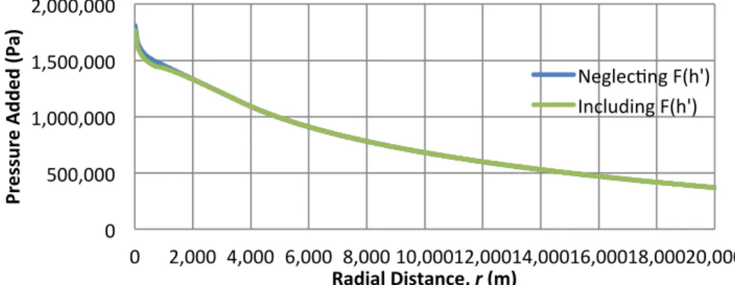
Figure 5 shows aquifer pressure increases verses radial distance with an aquifer thickness of 15 m. When the domain has relatively low aquifer permeabilities and
thicknesses (1)’s assumed conditions are met and 𝐹 ℎ! is negligible. This suggests that
-‐71000 -‐66000 -‐61000 -‐56000 -‐51000 -‐46000 -‐41000 0 2 4 6 8 10 12 14 16 18 20 D pF (Pa) Aquifer Mobility, l 0 100,000 200,000 300,000 400,000 500,000 600,000 0 2,000 4,000 6,000 8,000 10,000 12,000 14,000 16,000 18,000 20,000 Pr es su re Ad de d (P a) Radial Distance, r (m) Neglec2ng F(h') Including F(h')
when applying this model first check if 𝐹 ℎ! is negligible. If this is not the case, the injection site’s domain is not suitable for this analytical solution.
Figure 5. Pressure change vs. radial distance for CO2 injection into a 15m thick aquifer Use of Average Flow Rates
The CO2 pressure equation (1) was derived with the assumption that 𝑄!"## is a
constant CO2 flux. We can approximate effects from a changing flux by using an average.
The existing algorithm uses end of time-step leaky flow rates, 𝑄!"##,!, when writing the set
of linear equations (9). This technique will herein be referred to as the “End of Time-step Flux Solver” (ETS) method.
Figure 6 shows an example of a leaky well’s flux (represented by the blue line)
increasing with time. Multiplying 𝑄!"##,! (represented by the orange line) by t
overestimates the volume of fluidtransferred by a source if 𝑄!"##,! is greater than
𝑄!"##,!"#,! (represented by the green line).
Figure 6. Leaky well flow rate vs. time The set of linear equations should be written with respect to 𝑄!"##,!"#.
𝑝!,! = 𝑝!"#,!+ 𝐺!,!,!"##𝑄!"##,!"#,! ! !"#!!! + 𝐺!,!,!"## 𝑄!"##,!"#,! − 𝑄!"##,!"#,!!! !!! !"##!!!! (18) 0 500,000 1,000,000 1,500,000 2,000,000 0 2,000 4,000 6,000 8,000 10,000 12,000 14,000 16,000 18,000 20,000 Pr es su re Ad de d (P a) Radial Distance, r (m) Neglec2ng F(h') Including F(h')
The average volumetric flow rate equals the total fluid mass transferred by the leaky well segment, 𝑀!"##,!! , divided by the effective fluid density, 𝜌
!"", divided by the time, 𝑡.
𝑄!"##,!"#,!! = 𝑀!"##,!! /𝜌!""𝑡 (19)
Effective densities are needed because 𝑀!"##,!! may be composed of both CO2 and
brine. The total fluid mass transferred by the leaky well segment at the end of the time-step can be calculated by
𝑀!"##,!! = 𝑀
!"##,!!!!! + 0.5Δ𝑡 𝑄!"##,,!!!!! + 𝑄!"##,!! 𝜌!"" (20) where Δ𝑡 is time-step duration. Substituting (20) into (19) gives
𝑄!"##,!"#,!! = 𝑀
!"##!!!!,!+ 0.5Δ𝑡 𝑄!"##!!!!,!+ 𝑄!"##!,! 𝜌!"" /𝜌!""𝑡 (21) Subtracting the bottom by the top layer average flow rates gives
𝑄!"##,!"#,!− 𝑄!"##,!"#,!!!
= 𝑀!"##!!!!,!− 𝑀!"##!!!!,!!! + 0.5Δ𝑡 𝑄!"##!!!!,!+ 𝑄!"##!,!
− 𝑄!"##!!!!,!!!+ 𝑄!"##!,!!! 𝜌!"" /𝜌!""𝑡
(22)
Time-step constants 𝑐! and 𝑐! are defined as,
𝑐! =𝑀!"## !!!!,!− 𝑀 !"##!!!!,!!!+ 0.5Δ𝑡 𝑄!"##!!!!,!− 𝑄!"##!!!!,!!! 𝜌!"" 𝜌!""𝑡 (23) 𝑐! = 0.5Δ𝑡 𝑡 (24)
Using 𝑐! and 𝑐!, (22) can be written concisely as
𝑄!"##,!"#,! − 𝑄!"##,!"#,!!! = 𝑐! 𝑄!"##,!− 𝑄!"##,!!! + 𝑐! (25)
Substituting (25) into (18) gives the modified pressure equation for the “Average Flux Solver” (AS) method.
𝑝!,! = 𝑝!"#,!+ 𝐺!,!,!"##𝑄!"##,! ! !"##!! + 𝑐!𝐺!,!,!"## 𝜋𝑟!"!"##,!! 𝑘!"##,! 𝑘!,!"",!"##,! 𝜇!""𝐵! 𝑝!"##,!!! !!! !"##!!!! − 𝜌!𝑔𝐵! − 𝑔𝐻!!!(𝜌!− 𝜌!ℎ!,!!!! + 𝜌 !ℎ!,!!!! ) − 𝑝!"##,! − 𝜋𝑟!"!"##,!!!! 𝑘 !"##,!!! 𝑘!,!"",!"##,!!! 𝜇!""𝐵!!! 𝑝!"##,! − 𝜌!𝑔𝐵!!!− 𝑔𝐻!(𝜌! − 𝜌!ℎ!,!! + 𝜌 !ℎ!,!! ) − 𝑝!"##,!!! + 𝑐!𝐺!,!,!"## (26)
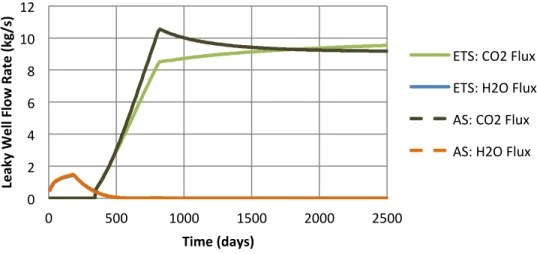
Figure 7 compares CO2 and brine leaky well flux rates verse time calculated using
the ETS and AS methods. In this case, leaky well CO2 flux is estimated to be greater when
using the AS method. Recall from (10) that Δp = G*Q. If Qt is greater than Qavg, the
change in pressure calculated by G* Qt will be greater than the change is pressure
calculated by G* Qavg. As a result, artificially low leaky well flow rates are estimated
when Qt > Qavg and the ETS method (G* Qt) is used to estimate pressure changes.
Figure 7. Leaky well flow rates vs. time
It is also important to note that in Figure 7 the steep increase in CO2 flux rates (t =
~400 - 800 days) occurs as a result of the rapidly increasing CO2 relative permeability in
the leaky well due to the increasing plume thickness. The slope of CO2 flux vs. time
abruptly lessens around t = 800 days when the CO2 relative permeability reaches unity (krc
= 1) and is unable to continue increasing.
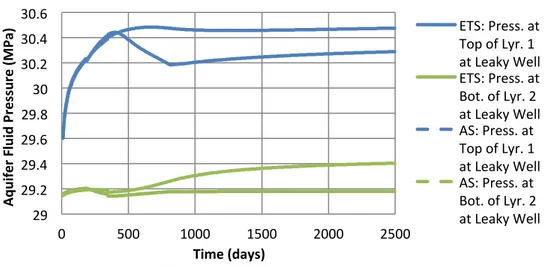
Aquifer fluid pressures at the leaky well determined using the ETS and AS methods are compared in Figure 8. Intuitively, pressures determined by the AS method seem
correct. The blue dashed line shows pressure in the lower aquifer building rapidly in the first 500 days then reaching a semi steady-state condition. The green dashed line shows
0 2 4 6 8 10 12 0 500 1000 1500 2000 2500 Le aky W el l Fl ow Ra te (kg /s ) Time (days)
ETS: CO2 Flux ETS: H2O Flux AS: CO2 Flux AS: H2O Flux
pressure in the top aquifer remaining low until sufficient pressure builds up in the bottom
aquifer and the relative conductivity of CO2 in the leaky well approaches unity. As seen in
Figure 7, the leaky well flux reaches a maximum once these conditions are met because of a build-up of pressure in the lower aquifer caused by earlier low relative conductivities. The leaky well flow rate begins to subside as the fluid pressure begins to increase in the top aquifer, reducing the pressure gradient across the aquitard.
Figure 8. Aquifer fluid pressures vs. time
Figure 8 also shows that aquifer fluid pressures are found to have less abrupt transitions through time when using the AS method. This is because the AS method directly accounts for the flow rate history when calculating end of time-step flow rates.
This analysis suggests that the AS method should always be used with applying this algorithm. The AS method multiplies the correct flow rate by the Green’s functions, gives smoother fluid pressure verse time profiles, and therefore provides a more accurate leakage estimation.
CO2 and Brine Separation
The existing algorithm takes the sum of the CO2 and brine flow rates to calculate
the total volumetric source or sink when determining Qwell for the pressure equation. This
technique will be referred to as the “Combined Flux” (CF) method. A “Separated Flux” (SF) method may improve this algorithm by eliminating the need to make assumptions concerning the discontinuous nature of (1) and effective phase dependent parameters, such as density, relative conductivity.
The SF method uses (1) to determine pressure added from CO2 leakage and the
Theis Equation, 𝑝!,!− 𝑝!"#,! = 𝜌!𝑔 4𝜋𝑇!𝑊 𝑢!,!,!"## 𝑄!,! (27) where, 𝑢!,!,!"## =𝑟!,!"## ! 𝑆 ! 4𝑇!𝑡 (28) 29 29.2 29.4 29.6 29.8 30 30.2 30.4 30.6 0 500 1000 1500 2000 2500 Aq ui fe r Fl ui d Pr es su re (MP a) Time (days)
ETS: Press. at Top of Lyr. 1 at Leaky Well ETS: Press. at Bot. of Lyr. 2 at Leaky Well AS: Press. at Top of Lyr. 1 at Leaky Well AS: Press. at Bot. of Lyr. 2 at Leaky Well
to determine pressure added from brine leakage. In (27) and (28) 𝑇! is the layer
transmissivity, 𝑊 𝑢 is the Well function, 𝑟!,!"## is the horizontal distance between well
‘w’ and well ‘well’, and 𝑆! is the layer storativity. The SF method modifies the
superpositioning of pressure sources as follows:
𝑝!,! = 𝑝!"#,!+ 𝐺!,!,!"##𝑄!,!"##,!+ 𝜌!𝑔 4𝜋𝑇!𝑊 𝑢!,!,!"## 𝑄!,!"##,! ! !"##!! + 𝐺!,!,!"## 𝑄!,!"##,!− 𝑄!,!"##,!!! !!! !"##!!!! +4𝜋𝑇𝜌!𝑔 ! 𝑊 𝑢!,!,!!"" 𝑄!,!"##,!− 𝑄!,!"##,!!! !!! !"##!!!! (29)
The definition of 𝑐! must be redefined and a similar term for brine, 𝑐!, must be created to
apply the AS method to the SF method.
𝑐! =𝑀! !!!!,!− 𝑀 !!!!!,!!!+ 0.5Δ𝑡 𝑄!!!!!,!− 𝑄!!!!!,!!! 𝜌!𝑡 (30) 𝑐! = 𝑀! !!!!,!− 𝑀 !!!!!,!!!+ 0.5Δ𝑡 𝑄!!!!!,!− 𝑄!!!!!,!!! 𝜌!𝑡 (31) 𝑝!,! = 𝑝!"#,!+ 𝐺!,!,!"##𝑄!,!"##,!+ 𝜌!𝑔 4𝜋𝑇!𝑊 𝑢!,!,!"## 𝑄!,!"##,! ! !"##!! + 𝑐!𝐺!,!,!"## 𝑄!,!"##,!− 𝑄!,!"##,!!! !!! !"##!!!! + 𝑐!𝐺!,!,!"## + 𝜌!𝑔 4𝜋𝑇! 𝑐!𝑊 𝑢!,!,!"#! 𝑄!,!"##,!− 𝑄!,!"##,!!! !!! !"##!!!! + 𝑐!𝑊 𝑢!,!,!"## (32)
𝑝!,! = 𝑝!"#,!+ 𝐺!,!,!"##𝑄!,!+ 𝜌!𝑔 4𝜋𝑇!𝑊 𝑢!,!,!"## 𝑄!,! ! !"##!! + 𝑐!𝐺!,!,!"## 𝜋𝑟!"!"##,!! 𝑘!"##,! 𝑘!" !"##,! 𝜇!𝐵! 𝑝!"##,!!!− 𝜌!𝑔𝐵! !!! !"##!!!! − 𝑔𝐻!!!(𝜌!− 𝜌!ℎ!,!!!! + 𝜌 !ℎ!,!!!! ) − 𝑝!"##,! − 𝜋𝑟!!!"##,!!!! 𝑘 !"##,!!! 𝑘!" !"##,!!! 𝜇!𝐵!!! 𝑝!"##,!− 𝜌!𝑔𝐵!!!− 𝑔𝐻!(𝜌! − 𝜌!ℎ!,!! + 𝜌 !ℎ!,!! ) − 𝑝!"##,!!! + 𝑐!𝐺!,!,!"## + 𝜌!𝑔 4𝜋𝑇! 𝑐!𝑊 𝑢!,!,!"## 𝜋𝑟!"!"##,!! 𝑘!"##,! 𝑘!" !"##,! 𝜇!𝐵! 𝑝!"##,!!! !!! !"##!!!! − 𝜌!𝑔𝐵!− 𝑔𝐻!!! 𝜌!− 𝜌!ℎ!,!!!! + 𝜌 !ℎ!,!!!! − 𝑝!"##,! − 𝜋𝑟!"!!"",!!!! 𝑘 !"##,!!! 𝑘!" !"##,!!! 𝜇!𝐵!!! 𝑝!"##,!− 𝜌!𝑔𝐵!!! − 𝑔𝐻! 𝜌!− 𝜌!ℎ!,!! + 𝜌 !ℎ!,!! −𝑝!"##,!!! + 𝑐!𝑊 𝑢!,!,!"## (33)
The SF method reduces the problem’s complexity in several ways. First, unlike the CF method, it becomes unnecessary to determine effective phase dependent parameters such as density, relative conductivity, and viscosity. We do not have to assume a method
for determining these effective parameters. In the SF method, the CO2 portion of Equation
(32) uses CO2’s relative conductivity and viscosity while the brine portion of Equation (32)
uses the relative conductivity and viscosity of brine.
In addition, it simplifies the complexity of calculating Green’s functions from Equation (1). Using the CF method, it quickly becomes difficult to choose between using
volumetric CO2 fluxes, Qc, and total volumetric flow rates, Qwell, when determining
discretization breaks. The SF method always uses CO2 volumetric flow rates when
calculating Green’s function values and brine volumetric flow rates when calculating Well function values.
Figure 9 shows the radial fluid pressure distribution for a single well injecting CO2
or brine into a confined aquifer for 2500 days. In both cases, either method produces
exactly the same fluid pressure distributions. Both methods use (1) in the case of pure CO2
flux, however, it is interesting to note that (1) I mimics (27) in the case of pure brine flux.
Figure 9. Aquifer pressure change vs. radial distance when individually injecting brine or CO2 -‐0.5 0.5 1.5 2.5 3.5 0 2,000 4,000 6,000 8,000 10,000 12,000 14,000 16,000 18,000 20,000 Pr es su re C ha ng e (MP a) Radial Distance (m)
CO2 Injec2on (Both Methods) H2O Injec2on (Both Methods)
Figure 10 shows the radial fluid pressure distribution for a single well injecting
both CO2 and brine. Both methods simulated a mixture of 50% CO2 and 50% brine (by
volume) being injected into a confined aquifer for 2500 days. While the fluid pressure changes converged at a distance of approximately 2.5 km, pressure changes estimated using the SF method were much higher than pressure changes calculated using the CF
method near the injection well. This is because if the radial distance is within the CO2
plume the CF method assumes that the total flux behaves as CO2 flux.
Figure 10. Aquifer pressure change vs. radial distance when simultaneously injecting both brine and CO2
Figure 11 shows the CO2 and brine leaky well flux rates verse time calculated using
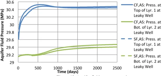
the CF and SF methods. Figure 12 compares fluid pressure in both layers at the leaky well over time between the CF and SF methods. Both algorithms also use the AS method.
Figure 11. Leaky well flow rates vs. time
Lower CO2 flux rates are calculated using the SF method because of a higher
pressure sensitivity to fluid flux. While the SF method initially predicts greater increases in fluid pressure in the bottom layer, leaky well flow rates cause greater increases in the top layer’s fluid pressure. This reduces the pressure gradient (Figure 12) resulting in less leakage. In other words, less leakage is needed to equalize the pressure differential between aquifer layers because the SF method estimates more pressure change per volumetric unit of leakage.
0.0 0.5 1.0 1.5 2.0 2.5 3.0 3.5 0 2,000 4,000 6,000 8,000 10,000 12,000 14,000 16,000 18,000 20,000 Pr es su re C ha ng e (MP a) Radial Distance, r (m)
CF: CO2 & Brine Inj. SF: CO2 & Brine Inj.
0 2 4 6 8 10 12 0 500 1000 1500 2000 2500 Le aky W el l Fl ow Ra te (kg /s ) Time (days)
CF,AS: CO2 Flux CF,AS: H2O Flux SF,AS: CO2 Flux SF,AS: H2O Flux
Figure 12. Aquifer fluid pressures vs. time Conclusions
This work has led to several important observations and recommendations
concerning the semi-analytical algorithm developed by Celia et. al. (2011) and Nordbotten
et. al. (2009). Interestingly, the CO2 pressure equation (1) provides exactly the same
pressure distribution at the Theis equation (27) in the case of pure brine flux. Steep
increases in leaky well CO2 flux rates occur as a result of the rapidly increasing relative
permeability due to increasing lower layer plume thicknesses. Also, CO2 flux rate
increases abruptly reduce when the relative permeability reaches unity.
There are two possibilities concerning the pressure offset term 𝐹 ℎ! . First, when
domains have relatively high aquifer permeabilities or thicknesses fundamental
assumptions are violated and the algorithm is rendered unsuitable. The second possibility occurs when domains have relatively low aquifer permeabilities and thicknesses. In this
case, (1)’s assumed conditions are met and 𝐹 ℎ! is negligible. A reasonable suggestion
based upon this work would be to first check if 𝐹 ℎ! is negligible. If this is the case,
proceed with the simulation using the semi-analytical model. Otherwise, the injection site’s domain is not suitable for the semi-analytical leakage model.
Changes in fluid pressure should be calculated by multiplying Green’s functions by average flow rates not end of time-step flow rates. Artificially low leaky well flow rates
have been estimated when Qt > Qavg and ETS method is used. In addition, aquifer fluid
pressures have smoother transitions through time using the AS method. This work’s results indicate that the AS method should always be used as it seems to produce more accurate flux rates and leakage values throughout the simulation duration.
Separating leaky well CO2 and brine fluxes and applying the Theis solution to
estimate pressure changes resulting from brine flow eliminating this model’s need to make assumptions concerning the discontinuous nature of (1) and effective phase dependent parameters, such as density, relative conductivity.
The SF method returns lower CO2 flux rates than the CF method. The reason for
this is less flux is needed to equalize the pressure differential between aquifer layers because the SF method estimates more pressure change per volumetric unit of leakage.
29 29.2 29.4 29.6 29.8 30 30.2 30.4 30.6 0 500 1000 1500 2000 2500 Aq ui fe r Fl ui d Pr es su re (MP a) Time (days)
CF,AS: Press. at Top of Lyr. 1 at Leaky Well CF,AS: Press. at Bot. of Lyr. 2 at Leaky Well SF,AS: Press. at Top of Lyr. 1 at Leaky Well SF,AS: Press. at Bot. of Lyr. 2 at Leaky Well
This method needs numerical modeling testing to verify fluid pressure responses however it shows promise in providing a more accurate solution.
Acknowledgements. The authors would like to thank the U.S. Department of Energy-NETL Office (Grant DE-FE0001830) for their continued support.
References
Celia, M. A., J. M. Nordbotten, B. Court, M. Dobossy, S. Bachu (2011). Field-scale application of a semi-analytical model for estimation of CO2 and brine leakage along old wells, International Journal of
Greenhouse Gas Control, 5: 257-269.
Nordbotten, J. M., D. Kavetski, M. A. Celia and S. Bachu (2009). Model for CO2 leakage Including Multiple
Geological Layers and Multiple Leaky Wells. Environmental Science & Technology, 43: 743-749. Nordbotten, J.M. and M.A. Celia (2006). Similarity solutions for fluid injection into confined aquifers. J.
Fluid Mech., 561: 307-327.
Nordbotten, J.M.; M.A. Celia and S. Bachu (2005a). Injection and Storage of CO2 in Deep Saline Aquifers:
Analytical Solution for CO2 Plume Evolution During Injection. Transp Porous Med, 58: 339-360.\
Nordbotten, J.M.; M.A. Celia and S. Bachu (2005b). Semianalytical Solution for CO2 Leakage through an
Abandoned Well. Environ. Sci. Technol., 39: 602-611.
Nordbotten, J.M.; M.A. Celia and S. Bachu. (2004). Analytical solutions for leakage rates through abandoned wells. Water Resources Research, 40. W04204, doi: 10.1029/2003WR002997.