This is an author produced version of a paper published in Remote Sensing of Environment. This paper has been peer-reviewed but does not include the final publisher proof-corrections or journal pagination.
Citation for the published paper:
Jamali, Sadegh; Jönsson, Per; Eklundh, Lars; Ardö, Jonas; Seaquist,
Jonathan. (2015). Detecting changes in vegetation trends using time series segmentation. Remote Sensing of Environment, vol. 156, p. null
URL: https://doi.org/10.1016/j.rse.2014.09.010
Publisher: Elsevier
This document has been downloaded from MUEP (https://muep.mah.se) / DIVA (https://mau.diva-portal.org).
Detecting Changes in Vegetation Trends using Time Series Segmentation
1 2 3
Sadegh Jamali a,*, Per Jönsson b, Lars Eklundh a, Jonas Ardö a, Jonathan Seaquist a 4
5
Affiliations: 6
7
a Department of Physical Geography and Ecosystem Science, 8
Lund University, Sölvegatan 12, SE-223 62 Lund, Sweden 9
10
b Division of Materials Science and Applied Mathematics, 11
Malmö University, Sweden 12 13 * Corresponding author: 14 15 Sadegh Jamali 16
Department of Physical Geography and Ecosystem Science 17 Lund University 18 Sölvegatan 12 19 SE-223 62 Lund 20 Sweden 21 Phone: +46 46 222 1725 22 Fax: +46 46 222 0321 23
E-mail: Sadegh.Jamali@nateko.lu.se 24
25
Keywords:
26
Vegetation dynamics, Change detection, Vegetation imagery, Trend analysis, Time series, 27
Segmentation, DBEST, GIMMS, NDVI 28 29 30 Abstract 31 32
Although satellite-based sensors have made vegetation data series available for several decades, 33
the detection of vegetation trend and change is not yet straightforward. This is mainly due to the 34
quality of the available change detection algorithms, which seldom meet users’ main need for 35
identifying and characterizing both abrupt and non-abrupt changes, without sacrificing accuracy 36
or computational speed. We propose a user-friendly program for analysing vegetation time 37
series, with two main application domains: generalising vegetation trends to main features, and 38
characterizing vegetation trend changes. This program, Detecting Breakpoints and Estimating 39
Segments in Trend (DBEST) uses a novel segmentation algorithm which simplifies the trend into 40
linear segments using one of three user-defined parameters: a generalisation-threshold parameter 41
δ, the m largest changes, or a threshold β for the magnitude of changes of interest for detection.
42
The outputs of DBEST are the simplified trend, the change type (abrupt or non-abrupt), and 43
estimates for the characteristics (time and magnitude) of the change. DBEST was tested and 44
evaluated using simulated Normalized Difference Vegetation Index (NDVI) data at two sites, 45
which included different types of changes. Evaluation results demonstrate that DBEST quickly 46
and robustly detects both abrupt and non-abrupt changes, and accurately estimates change time 47
and magnitude. 48
49
DBEST was also tested using data from the Global Inventory Modeling and Mapping Studies 50 (GIMMS) NDVI image time series for Iraq for the period 1982-2006, and was able to detect and
51 quantify major change over the area. This showed that DBEST is able to detect and characterize changes over large areas. We conclude that DBEST is a fast, accurate and flexible tool for trend 53
detection, and is applicable to global change studies using time series of remotely sensed data 54 sets. 55 56 57 1. Introduction 58 59
Vegetation is an important component of terrestrial ecosystems (e.g. Prentice et al., 2000; Sitch 60
et al., 2003). It is now widely recognized that vegetation can respond to climate and disturbance 61
in a complex, non-linear fashion (e.g. Lambin and Ehrlich, 1997). External disturbances to 62
ecosystems, including insect outbreaks, fires, forest clear-cutting, and conversion of natural 63
grasslands to cultivated crops, increase the complexity of vegetation variations across a wide 64
range of spatio-temporal resolutions and scales (e.g. Higgins et al., 2002; Lambin et al., 2003). 65
There is a corresponding need for data and tools which can properly capture and represent such 66
complex dynamics, at a level of detail which is appropriate to the question under consideration. 67
One flexible and simplifying idea is to allow the user to define the boundary between signal and 68
noise. Developing analysis tools that embody this idea can help us to characterize and understand 69
vegetation dynamics with much greater efficiency. 70
71
Vegetation dynamics are often monitored at different spatial and temporal scales through 72 vegetation index data series, such as GIMMS (Global Inventory Modeling and Mapping
73
Studies), MODIS (Moderate Resolution Imaging Spectroradiometer), and SPOT/Vegetation
74
(System Pour l’Observation de la Terre) data sets. One widely used index is the Normalized
75
Difference Vegetation Index (NDVI), which is an indicator of the vegetation’s greenness (Rouse 76
et al., 1973). Temporal trend analysis of NDVI has proved particularly useful for monitoring and
77
characterizing the response of land cover to phenomena with a range of time scales, from abrupt
78
natural or anthropogenic events (Verbesselt et al., 2009), to seasonal variability of plant
79
phenology caused by changes in temperature and rainfall regimes (Heumann et al., 2007),
80
through to gradual inter-annual climate changes (Jacquin et al., 2010). Similar analyses of NDVI 81
trends have also been used to investigate the relationship between NDVI and Leaf Area Index 82
(LAI), a key variable which is functionally related to plant biomass production. Studies have 83
indicated that this relationship is not completely linear, particularly for high LAI values (e.g. 84
Carlson and Ripley, 1997; Fan et al., 2009). 85
86
Non-linear temporal trends in NDVI can be studied by a number of techniques, including time 87
series segmentation (Keogh et al., 2004). Series segmentation refers to approximating a time 88
series by a set of piecewise straight-line segments, in the process eliminating noise but 89
preserving the salient details of the trend. Two significant merits of segmentation are that first, it 90
approximates complex signatures to extract their basic features (Zeileis et al., 2003) and second, 91
it increases the efficiency of data storage and further computation (Keogh et al., 2004). The size 92
of the output set can vary between one and the size of the original time series, and is a key 93
parameter in determining the type of information available to the user, from most 94
generalised/compressed information (one segment) to all possible details (all data points). 95
96
A particular type of segmentation technique, which always outputs one segment, is the ordinary 97
least squares (OLS) technique. It has been widely used for assessing long-duration changes in 98
vegetation greenness using NDVI time series (Fuller, 1998; Eklundh and Olsson, 2003; Nemani 99
et al., 2003; Fensholt et al., 2009; Peng et al., 2012). However, the implicit assumption that 100
vegetation always changes gradually and constantly over the entire study period is a critical 101
drawback of this method (e.g. Jamali et al., 2014). Consequently, it is impossible using OLS to 102
identify periods in which the rate of change, or even the sign of the rate of change, varies within 103
a given time period: for example, the existence of short-duration nonlinearities such as 104
‘greening’ or ‘browning’ patterns may be completely obscured because they have been averaged 105
out altogether (de Jong et al., 2012). On the other hand, using the original time series in further 106
analysis is not cost effective and may also, in cases when only the main features of the vegetation 107
change are of interest, carry unused detailed information and noise. 108
109
Fortunately, to date at least two alternative approaches between the two mentioned extreme cases 110
have been introduced for detecting trends and estimating changes in vegetation time series. The 111
first approach, Landsat-based Detection of Trends in Disturbance and Recovery (LandTrendR), 112
uses arbitrary temporal segmentation to divide long-term trends into piecewise linear segments 113
for the representation of spectral change in forested ecosystems (Cohen et al., 2010; Kennedy et 114
al., 2010). LandTrendR focuses solely on Landsat derived data, and requires several complex 115
properties of different instruments may require alteration of the algorithms and parameters used 117
in LandTrendR, and its generalisation for use with time series of other sensors in other ecosystems has not yet been implemented.
119 120
The second approach, Breaks For Additive and Seasonal Trend (BFAST), was one of the first 121
general methods for detecting changes in time series data, focusing on the trend and seasonal 122
components in long term NDVI data series, at spatial scales ranging from continental to global 123
(e.g. Verbesselt et al., 2010a; Verbesselt et al., 2010b; de Jong et al., 2012; de Jong et al., 2013). 124
It employs a generic approach by assuming that a time series can be modelled in terms of its 125
trend, seasonal, and remainder components, including breaks in the trend and seasonal 126
components. In BFAST, nonlinearity in the trend component is also simplified into a number of 127
individual trend segments, in order to identify sudden structural shifts. The simplified trend is 128
therefore composed of segments with gradual changes, separated from each other by relatively 129
brief, abrupt changes (Verbesselt et al., 2010a; de Jong et al., 2012; de Jong et al., 2013). Our 130
experience using BFAST (most recent version 1.4.4) shows that although the user can control the 131
number of breaks to be detected, they do not have full control over the level of trend 132
generalisation (whether basic features or detailed information will be extracted), or over the 133
change magnitude that is detected. More importantly, the requirement that gradual changes are 134
separated from each other by a sudden change (most often with a duration of one time step) may 135
not always guarantee the best approximation of trend nonlinearity for real-world data, where 136
changes of different types and durations may exist. 137
Thus, to the best of our knowledge, no attention has yet been paid to segmenting time series of 139
vegetation indices to generalise trends and detect both abrupt and non-abrupt changes, in a way 140
which allows the user to control the segmentation. Ideally the user should be able to choose the 141
generalisation scheme and extract information about both the main feature and details. The user 142
should also be able to detect and characterize changes of interest, including realistic abrupt and 143
non-abrupt changes of different durations and in any order within a particular sequence of 144
occurrences. 145
146
The overall aim of this paper is to propose a novel approach for segmenting and analysing trend 147
changes in time series of vegetation indices (VI). The method, called Detecting Breakpoints and 148
Estimating Segments in Trend (DBEST), provides both generalised trend segments and estimates 149
of the characteristics of both abrupt events and long-term processes. DBEST has been tested and 150
evaluated using simulated NDVI data series. We also applied DBEST to a GIMMS-NDVI 151
dataset (1982-2006) for Iraq, to detect major changes, determine change type (abrupt or non-152
abrupt) and estimate the characteristics (time, magnitude) of the changes in a spatio-temporal 153
framework. The method allows for fast, flexible and accurate estimations of trends, essential 154
from a global change perspective. 155
156 157
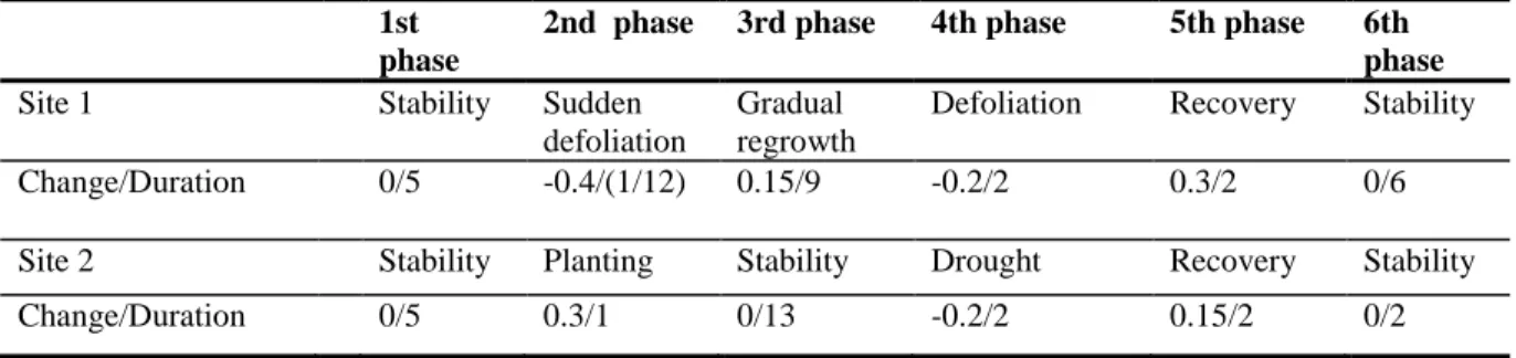
2. Data and study area
158 159
We have developed our method using a commonly used time-series data source: the NASA 160
GIMMS data set. Then, we applied the methods to selected study areas that highlight certain 161
temporal features. The methods are not specific to either the data type or the sites, which merely 162
represent commonly used data and illustrative cases. 163
164
2.1. GIMMS data
165 166
The GIMMS data set is a twice-monthly composite NDVI product with global coverage at an 8-167
km spatial resolution, which is available for the 25.5 year period from July 1981 to December 168
2006 (Tucker et al., 2004; Tucker et al., 2005). The GIMMS data were derived from the output 169
of the AVHRR (Advanced Very High Resolution Radiometer) instrument on board NOAA 170
(National Oceanographic and Atmospheric Administration) satellite series 7, 9, 11, 14, 16 and 171
17. The NDVI is computed from the red and near infrared bands of the AVHRR sensor, and is 172
correlated with photosynthetic activity and the LAI of green vegetation. The GIMMS data have 173
been corrected for variations arising from calibration, view geometry, volcanic aerosols, and 174
other factors not related to actual vegetation change (Tucker et al., 2005). The GIMMS data have 175
also been validated against the well-calibrated and atmospherically-corrected MODIS data set 176
for the period 2000-2007, and for the Earth’s semi-arid regions (Fensholt et al., 2012). Despite 177
the corrections, the GIMMS data may contain residual invalid measurements, but these are well 178
indicated using quality flags (de Jong et al., 2012). Based on the quality flags, we only 179
considered pixels with at least 75% valid data points (i.e., flag value zero) through the whole 180 time span. 181 182 2.2. Study area 183 184
The case study was Iraq, selected due to the fact that large parts of the county’s land surface have 185
undergone major changes in the recent past. Iraq’s geography consists of four main zones: desert 186
in the west and southwest, rolling upland between the upper Tigris and Euphrates rivers in north 187
central Iraq, highlands in the north and northeast with mountains, and alluvial plain through 188
which the Tigris and Euphrates flow from northwest to southeast. About 77.7% of Iraq’s land 189
area is not viable for agriculture. 0.3% is forest and woodlands situated along the extreme 190
northern border with Turkey and Iran. The remaining 22% are used for a range of agricultural 191
activities (Schnepf, 2004). 192
193
Over the last two to three decades, the landscape of Iraq has witnessed many changes (UNEP, 194
2001). These have been caused by frequent natural hazards, such as sand storms (Draxler et al., 195
2001) and floods (Hamdan et al., 2010), and human activities, such as forced migration, social 196
conflicts, and wars (especially in south-eastern and northern Iraq). The high probability of abrupt 197
vegetation disturbances and recoveries made Iraq the ideal study area to test DBEST. 198 199 200 3. Methods 201 202
In this section, DBEST algorithm is introduced, and then approaches used for validating and 203
evaluating DBEST’s performance are explained. The DBEST algorithm consists of two main 204
parts: trend estimation and trend segmentation. 205
206
3.1. The trend estimation method
208
For a given VI time series (including seasonal variations), the temporal trend is derived using the 209
Seasonal-Trend decomposition procedure based on Loess (STL) (Cleveland et al., 1990), 210
implemented in an unpublished version of the TIMESAT software package (Jönsson and 211
Eklundh, 2004). STL is a fast filtering procedure able to deal with missing values, for 212
decomposing a time series into trend (low frequency variation), seasonal (variation at or near the 213
seasonal frequency), and remainder (remaining variation) components. TIMESAT is a software 214
package for analysing time series of satellite sensor data, which makes it possible to investigate 215
the seasonality of the data and their relationship with dynamic properties of vegetation such as 216
phenology. 217
218
Before using STL, the existence of significant discontinuities in the VI level is examined. To do 219
this, the absolute difference in VI between each pair of consecutive data points, starting from the 220
time series’ start point, is compared with a user-defined first level-shift-threshold (θ1). If the 221
absolute difference is greater than the threshold value, a second criterion tests whether the 222
change led to a significant shift in the mean VI level which persists throughout a user-defined 223
time period, the duration-threshold (ϕ). The second criterion is valid if the absolute difference in 224
the means of the VI data, calculated over a period ϕ before and after the current data point, is 225
greater than a user-defined second level-shift-threshold (θ2).
226 227
If both tests are valid, the current data point is marked as a candidate level-shift point. The same 228
procedure is repeated for every data point in the time series. The candidate points are then sorted 229
into descending order according to the absolute value of the shift in the VI level. The first point 230
in the sorted list is marked as the most significant level-shift point. For the second and 231
subsequent candidate points, in addition to the two mentioned criteria, a third criterion should be 232
fulfilled in order to be marked as the next significant level-shift points. The third criterion checks 233
if the spacing between the candidate point and any previously detected level-shift point is at least 234
the duration-threshold ϕ. Bai and Perron (2003) and Zeileis et al. (2003) also recommend a 235
fraction of data needed between successive breaks. At any detected level-shift point, the VI time 236
series is divided into two parts, before and after. 237
238
The STL decomposition is then performed separately for each part of the time series divided by 239
the detected level-shift points (called hereafter separate STL decomposition) if one or more 240
level-shift points have been detected: if no such points are found, it is performed once for the 241
entire time series. The separate STL decomposition procedure often results in more precise trend 242
and seasonal components (especially around the detected level-shift points) because the shifts in 243
the VI level are not deformed by the smoothing methods used in the STL method (Cleveland et 244
al., 1990). 245
246
If the given time series is already deseasonalized (i.e. we are examining the trend component) 247
then significant level-shifts are similarly detected but of course no STL decomposing is needed. 248
249
3.2. The segmentation method
250 251
For the trend time series (either computed using the STL or already deseasonalized), with a 252
number of observations N (N>2), single time-step differences in the forward and backward 253
directions are calculated at every time-point i (2 ≤ i≤ N-1), as follows (Fig. 1a): 254 255 𝛥𝑉𝐼(𝑖−1,𝑖)= (𝑉𝐼(𝑖)− 𝑉𝐼(𝑖−1)) (1) 256 𝛥𝑉𝐼(𝑖,𝑖+1)= (𝑉𝐼(𝑖+1)− 𝑉𝐼(𝑖)) (2) 257 258
For each point i the peak/valley detector function (𝑓) is then computed, based on the continuity 259
of the sign of the two differences: 260 261 𝑓(𝑖) = {1, if sign(𝛥𝑉𝐼(𝑖−1,𝑖)) = −sign(𝛥𝑉𝐼(𝑖,𝑖+1)) 0, otherwise (3) 262 263
As specific cases, the peak/valley detector function is set to one at the start point (i=1) and zero 264
at the end point (i=N) of the time series. The signum function sign(x) equals +1 for x greater than 265
zero, -1 for x less than zero, and zero for x equal to zero. Clearly, the trend direction changes at 266
time points at which the peak/valley detector function equals one (except the time series’ start 267
point). These points are called peak and valley points. 268
269
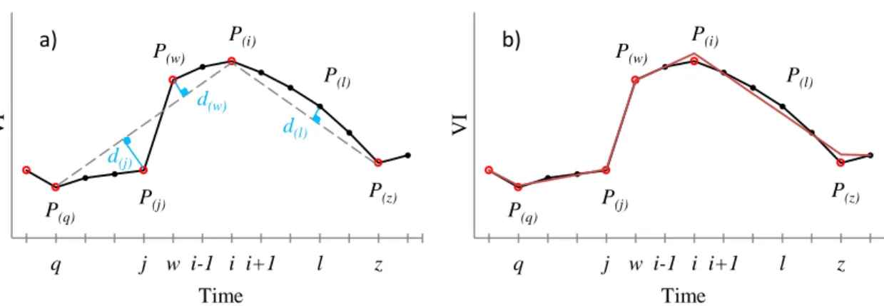
For all points of the time series, a second turning point detector function (𝑔), is computed based 270
on the peak/valley detector function and an iterative criterion, explained as follows. In first 271
iteration, for every pair of successive peak or valley points (e.g. P(q) and P(i) or P(i) and P(z) in Fig. 272
1a), a straight line passing through the two points is computed. Perpendicular distances (d) are 273
computed from all the intermediate non-peak and non-valley points (f=0) to the derived line. On 274
each side of the line (above and below), the intermediate point with maximum perpendicular 275
distance (e.g. P(j), P(w), P(l)) is selected, and this distance is compared with a user-defined 276
distance-threshold (ε), to be discussed later. If the distance is greater than the threshold (e.g. dj>ε 277
and dw>ε), the turning point detector function equals one (𝑔=1) at the selected point (i.e. P(j) and 278
P(w)), otherwise it is zero (𝑔=0) (e.g. P(l) with dl< ε). At non-selected points, the turning point 279
detector function equals zero as well. So the criterion is fulfilled only at the farthest points above 280
or below the line, provided that its perpendicular distance is above the threshold value. 281
282
𝑔(𝑖) = {
1, if 𝑓(𝑖) = 1
1, if 𝑓(𝑖) = 0 and the criterion is fulfilled. 0, if 𝑓(𝑖) = 0 and the criterion is not fulfilled.
(4) 283
284
As special cases, the first straight line passes through the time series’ start point and the first 285
peak or valley point; similarly the last line passes through the last peak or valley point and the 286
time series’ end point. For the second iteration, for every pair of successive points at which 𝑔=1, 287
a new straight line passing through the two points is computed and the rest proceeds exactly as 288
for the first iteration. The second iteration may add some new points to the set of points at which 289
𝑔=1. This same procedure is repeated for further iterations, until no new points with 𝑔=1are 290
detected. 291
292
Hereafter, time points at which the turning point detector function equals one (𝑔=1) are called 293
turning points: the set of turning points comprises the time series’ start point, the peak and valley
294
points and the points at which the criterion is fulfilled (Fig. 1). If u is the number of turning 295
points found for a given time series, then larger values of u indicate more peaks and valleys 296
and/or more points fulfilling the criterion in the trend time series. The turning points’ positions 297
(except the time series’ start point) indicate times when trend changes occur. Nevertheless, all 298
the u turning points are not necessarily associated with substantial changes. As will be discussed 299
later, the user can select changes that have considerable magnitude, after which the significance 300
of the turning points is tested from the fit quality standpoint. 301
302
Significant turning points are defined as turning points that significantly reduce the residual sum 303
of squares of a least-square fit to the VI trend time series (explained in next paragraph) and do 304
not result in over-fitting. The number of significant turning points can be determined by 305
minimizing an information criterion. The Bayesian Information Criterion (BIC) (Schwarz, 1978) 306
is a criterion for optimal model selection among a finite set of models. When computing the 307
least-squares fit, adding more turning points reduces the residual sum of squares but also 308
increases the number of model parameters, which may result in over-fitting problem. Both BIC 309
and the Akaike Information Criterion (AIC) (Akaike, 1974) resolve this problem by introducing 310
a penalty term for the number of parameters in the model. We have chosen the BICbecause it 311
has been argued that the AIC usually overestimates the number of breaks, while BIC is a suitable 312
selection in many situations (e.g. Zeileis et al., 2002; Zeileis et al., 2003). Given a finite set of 313
estimated models, the preferred or optimal model is the one with the lowest BIC value. 314
315
Before using BIC, the trend local change function, designated ℎ and defined in Eq. (5), 316
computes the difference in VI trend between successive turning points, and assigns it to the 317
current turning point: it is zero otherwise for non-turning points. For all points of the time series 318
the function h is defined as follows: 319 320 ℎ(𝑖) ={𝑉𝐼0, if 𝑔(𝑖) = 0 (𝑧)− 𝑉𝐼(𝑖), if 𝑔(𝑖) = 1 (5) 321
where i and z are the indices of the current and next turning points respectively. As two 322
exceptions, we choose z=N for computing ℎ for the last turning point, and z=2 for computing ℎ 323
for the first turning point (which is the time series’ starting point). All u turning points are then 324
sorted into descending order according to the magnitude of their trend local change (i.e. absolute 325
value of ℎ). The least-squares fit to the VI trend time series is computed for the entire time 326
series. The fitting is started with no turning point selected from the list to be considered in the fit 327
(i.e. linear fit), and then is repeated for cases where different numbers of the sorted turning points 328
(from just the first, to all u of them) are included in the fit. The BIC is computed for the fit 329
obtained for each case. The significant turning points are specified as the s (s ≤ u) points for 330
which the corresponding fit minimizes the BIC. 331
332
The least-squares fit to the trend time series is computed using the selected turning points, fitting 333
either one single straight-line (when no turning point is selected) or a composite line (when one 334
or more are selected). In computing the composite line, each selected turning point and the next 335
turning point after it in the trend time series are treated as data points to be shared by the 336
adjoining linear segments. This fitting method leads to a continuous, piecewise trend composed 337
of linear segments. Piecewise linear modelling, as a special case of non-linear regression 338
(Venables and Ripley, 2002), is often used to approximate complex phenomena and extract the 339
basic features of the data (Zeileis et al., 2003; Verbesselt et al., 2010). 340
341
The least-squares fitting is explained based on an example. Consider Fig. 1b with 14 data points, 342
where q=2, j=5, w=6, i=8, and z=13. The 𝑃(𝑞), 𝑃(𝑗), 𝑃(𝑤), 𝑃(𝑖), and 𝑃(𝑧) turning points are here 343
assumed as data points shared by adjoining segments. The composite line consists of six 344
segments (number of the assumed turning points plus one) and is obtained from the following 345 regression model (6). 346 347 𝑉𝐼(1)+ 𝜀1 = 𝑏 348 𝑉𝐼(2)+ 𝜀2 = 𝑎1+ 𝑏 349 𝑉𝐼(3)+ 𝜀3 = 𝑎1+ 𝑎2+ 𝑏 350 𝑉𝐼(4)+ 𝜀4 = 𝑎1+ 2𝑎2+ 𝑏 351 𝑉𝐼(5)+ 𝜀5 = 𝑎1+ 3𝑎2+ 𝑏 352 𝑉𝐼(6)+ 𝜀6 = 𝑎1+ 3𝑎2+ 𝑎3+ 𝑏 353 𝑉𝐼(7)+ 𝜀7 = 𝑎1+ 3𝑎2+ 𝑎3+ 𝑎4+ 𝑏 354 𝑉𝐼(8)+ 𝜀8 = 𝑎1+ 3𝑎2+ 𝑎3+ 2𝑎4+ 𝑏 355 𝑉𝐼(9)+ 𝜀9= 𝑎1+ 3𝑎2+ 𝑎3+ 2𝑎4 + 𝑎5+ 𝑏 356 𝑉𝐼(10)+ 𝜀10 = 𝑎1+ 3𝑎2+ 𝑎3+ 2𝑎4 + 2𝑎5+ 𝑏 357 𝑉𝐼(11)+ 𝜀11 = 𝑎1+ 3𝑎2+ 𝑎3+ 2𝑎4 + 3𝑎5+ 𝑏 358 𝑉𝐼(12)+ 𝜀12 = 𝑎1+ 3𝑎2+ 𝑎3+ 2𝑎4 + 4𝑎5+ 𝑏 359 𝑉𝐼(13)+ 𝜀13 = 𝑎1+ 3𝑎2+ 𝑎3+ 2𝑎4 + 5𝑎5+ 𝑏 360 𝑉𝐼(14)+ 𝜀14 = 𝑎1+ 3𝑎2+ 𝑎3+ 2𝑎4 + 5𝑎5+ 𝑎6+ 𝑏 361 362
Rewriting the model in matrix form and utilizing standard methods (Press et al., 1990) gives the 363
values of the coefficients 𝑎1, 𝑎2, 𝑎3, 𝑎4, 𝑎5 and 𝑎6 (slopes of the six linear segments) and 𝑏 364
(model value at the starting data point). Note that the composite line is continuous, but it does 365
not necessarily pass through the turning points considered in fitting. 366
367
The s significant turning points, which minimise the BIC, are called breakpoints. Note that the 368
significant breakpoints, as a subset of the turning points, can be abrupt (i.e. level-shift) or non-369
abrupt. The breakpoint detection method explained here can therefore be seen as more general 370
than methods in which only abrupt changes are detected, such as standard sequential test-based 371
methods used particularly in econometrics (Bai and Perron, 2003). 372
373
The next step allows the user to select either all breakpoints or a subset of them for output fit. 374
The selection depends on the reason for segmentation. If the reason is trend generalisation, there 375
are three options for the selection. If the required trend should reflect only a specified number m 376
(0 ≤ m≤ s) of the greatest changes (first option), the first m breakpoints having the largest 377
magnitude of the trend local change are selected. If the trend should contain segments with 378
variations equal to or lower than the user-defined threshold β (second option), then the k 379
breakpoints with change magnitudes larger than β are selected. The third option is to simplify the 380
trend up to a user-defined level (generalisation-threshold δ), compared to the least simplified 381
trend fit derived using all s breakpoints as the base level. In this case, the first r (r=ceil (s - 382
δ×0.01×s)) breakpoints are selected.
383 384
Alternatively, if the reason for segmentation is the detection and characterization of changes 385
(either the m greatest changes, or all changes greater than the magnitude β), then as another field 386
application of the segmentation algorithm, all detected breakpoints (s) will be selected to be 387
considered in the output fit. The user can choose a larger m (or lower β or lower δ) if their 388
interest is in trend details or short local events, or choose a smaller m (or higher β or higher δ) if 389
their interest is in the main features of the trend, or long-duration processes. 390
391
Finally, the least-squares fit to the trend time series (output fit) is computed using the selected 392
breakpoints, fitting either a straight-line (when m=0 or k=0 or r=0) or a composite line (when m 393
≥ 1 or k ≥1 or r≥1). The outputs of the trend generalisation algorithm are the generalised trend, 394
number of segments, and fit quality measures (root-mean-square-error (RMSE) and maximum-395
absolute-difference (MAD)). For any detected change, the time of the corresponding breakpoint 396
(which is called the break date) is considered to be the start time, and the time of the next turning 397
point in the trend time series is considered to be the end time. The change duration is the time 398
between the start and end times, and the change value is estimated by subtracting the fitted VI at 399
the start time from the fitted value at the end time. The sign of the change value indicates the 400
change direction, whether the slope is increasing or decreasing. The change type output denotes 401
whether the detected change is abrupt or non-abrupt dependent on whether the corresponding 402
breakpoint is a level-shift point or not, respectively. 403
404
An overview of DBEST is shown in Fig. 2, including some practical examples. For instance, in 405
order to generalise a trend time series at maximum level (fit one segment), set δ=100% in the 406
generalisation algorithm: the rest of the analysis is performed as explained above (Fig. 2, left 407
panel, Example 1). As a second example, to generalise the trend into main segments including 408
only one major breakpoint, set m=1 (Fig. 2, left panel, Example 2). Thirdly, to generalise into 409
segments containing variations ≤ 0.2 in NDVI units, set β=0.2 (Fig. 2, left panel, Example 3). 410
Obviously, setting β=0 or m=s or δ=0 leads to the least generalised form of the trend (i.e. fit 411
derived using all the s breakpoints). As an example for the change detection algorithm, to detect 412
the three major changes set m=3 (Fig. 2, right panel, Example 4). Here, all the s breakpoints are 413
used in the fitting, but the outputs are characteristics of only the three changes of interest. This 414
method, which can specify the changes of interest through either the change number or 415
magnitude parameters, preserves the highest fitting quality as well as the actual shape of the 416
change, because the output fit is composed of all significant segments. 417
418
As mentioned, the distance-threshold (ε) is a user-defined parameter, which can be set to a value 419
between zero and maximum absolute difference between data values of the given time series 420
(two for NDVI). However, values larger than the maximum influential value have no effect on 421
the segmentation process. By the maximum influential value we mean the value that if any 422
greater value than it is used for the distance-threshold, no turning points through fulfilling the 423
distance criterion is detected; only peak and valley points plus time series’ start point will be 424
detected as turning points (minimum possible u). The lower the value of ε relative to the 425
maximum influential value, the larger the number of turning points (u) that will be detected. 426
Setting ε=0 causes all data points to be detected as turning points (maximum possible u). A 427
default value for ε, however, is estimated in DBEST as follows: 428
429
𝜀 = 3𝑅∗ (7)
430 431
where 𝑅∗ is the root mean square error for the fit obtained using the peak and valley points plus 432
the time series’ start point (i.e. the distance-threshold is initially set to the maximum absolute 433
difference value). Interpretation of the estimated ε is that it is a statistical boundary (α=0.99) 434
between outlier and normal residuals of the obtained fit. This means that data points with outlier 435
residuals will most likely be detected as turning points through fulfilling the distance criterion, 436
and data points with normal residuals will not be detected. Hence, it is unlikely that noise leads 437
to false detection of turning points because they normally correspond to small residuals. 438
439
3.3. Validation
440 441
DBEST must be tested against remotely sensed satellite imagery in order to investigate its 442
reliability. However, as Verbesselt et al. (2010a) note, the validation of change detection 443
methods is not straightforward. This is frequently due to the unavailability of independent 444
reference sources for a wide range of potential changes during the change interval, and also 445
because the type and number of changes detected are never represented by field validated single-446
date maps (Kennedy et al., 2007). We therefore simulated NDVI data influenced by different 447
biophysical driving processes and events (both strengthening and disturbing plant greenness, 448
with both abrupt and gradual changes), and different types of plant response, in order to test 449
DBEST robustly under unambiguous and controlled conditions. In addition to using simulated 450
data, validation based on actual satellite data remains necessary because of the challenges 451
existent in perfectly simulating a real environment. Our satellite data were taken from Iraq, 452
where major changes in the NDVI have been observed (Hamdan et al., 2010; Richardson et al., 453
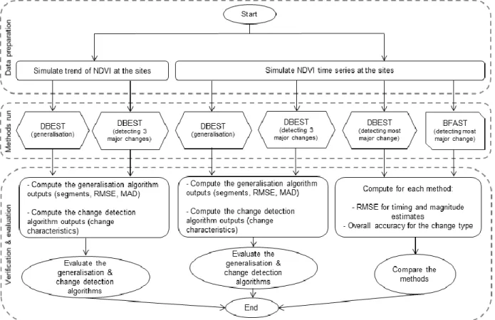
2005). Fig. 3 illustrates the overall workflow of the validation and evaluation processes. 454
455
3.3.1. Simulation 456
We simulated both NDVI trends (without seasonal cycles) and NDVI time series (including 458
seasonal cycles) at two sites with different biomes (forest at site 1 and cropland at site 2) for a 459
period of 300 months (corresponding to the real GIMMS data in Iraq) by using artificial 460
processes or events (with typical pre- and post-event life phases) and noise (Table 1). We 461
specified NDVI changes and their durations for each phase, based on observations of 462
corresponding biomes in real conditions. 463
464
At site 1, we considered two typical disturbance events in a series of six phases: a stable 465
condition followed by a sudden defoliation (causing a significant level-shift in NDVI), a gradual 466
re-growth phase, a second defoliation, a recovery phase, and finally a return to stable plant 467
greenness in the last phase. At site 2, one plantation and one drought, both with significant 468
impacts on NDVI, were used in respectively second and fourth phases just after stable conditions 469
in first and third phases. Similarly to site 1, a recovery phase and finally a return to stable plant 470
greenness were considered in respectively fifth and sixth phases (Table 1). 471
472
DBEST works for both types of trend (non-seasonal) and VI time series (including seasonal 473
cycles). We therefore simulated both types of data series. For each site, we simulated NDVI 474
trend data by computing a straight-line segment for each phase using an appropriate change and 475
duration to calculate the segment’s slope and intercept (Table 1). The initial NDVI levels, as 476
starting points in the first phases, were assumed to be 0.6 (site 1) and 0.15 (site 2). For generating 477
noise – which often originates from geometric and atmospheric errors in satellite data – we used 478
a random number generator with a zero-mean (μ=0) normal distribution and different values (at 479
least three) for standard deviation (σ = 0.01, 0.04, 0.07 NDVI units), corresponding to different 480
noise levels (low, medium, strong respectively) (Lhermitte et al., 2011; Roderick et al., 1996). 481
The generated noise for each level was then separately summed with the computed trend at each 482
site. Finally, the derived trends including high frequency variations were smoothed using a 483
locally-weighted regression (loess) smoother (Cleveland and Devlin, 1988) after which likely 484
level-shifts were detected. As recommended for the STL model (Cleveland et al., 1990), we used 485
a first degree polynomial model for the loess smoothing (with a smoothing span of 23 divided by 486
the total number of data points within each part of the time series). For evaluation purposes, the 487
NDVI trends were simulated with 500 iterations for each level of noise at each site. 488
489
To generate VI time series with seasonal trends and different types of noise, we simulated 490
seasonal periodic cycles of NDVI at each site, and added them to the earlier simulated noisy 491
trends (before applying the loess smoothing). Finally, we used the separate STL procedure 492
(θ1=0.1, θ2=0.2 NDVI units and ϕ=24 monthly time steps) to detect likely level-shifts and extract 493
trend components. In order to simulate the seasonal component for each biome, we used a 494
symmetric Gaussian function with amplitudes of maximum 0.2 (site 1) and 0.25 (site 2) for 495
healthy seasons. The maximum values were derived by using the STL function for some real 496
forest and cropland GIMMS-NDVI time series from the study area, extracting their seasonal 497
components, and approximating the amplitudes. The Gaussian type function has performed well 498
when used to calculate seasonality parameters by fitting the function to NDVI time series 499
(Jönsson and Eklundh, 2002). The amplitude values used for simulating the disturbed seasons 500
and seasons in the first phase at site 2 were assumed to be lower than the corresponding values 501
for healthy seasons. 502
3.3.2. Spatial application of the major change characterization
504 505
We generated monthly NDVI image series for a period of 25 years (1982-2006) by converting 506
the original twice-monthly GIMMS-NDVI data (25×12×2=600 images) to monthly data (300 507
images) using the maximum-value composite (MVC) method (Holben, 1986), which is similar to 508
the method used in GIMMS. Although the compositing method can reduce cloud and other noise 509
effects, the conversion was solely made because of the easier interpretation of monthly over 510
twice-monthly results, and is not a prerequisite for DBEST. The temporal trend of the monthly 511
NDVI data series was derived using the separate STL decomposition procedure (θ1=0.1, θ2=0.2 512
NDVI units and ϕ=24 monthly time steps). We then applied DBEST’s change detection 513
algorithm to the trends of the monthly NDVI data series in Iraq in order to detect, estimate, and 514
map major change characteristics (change type, timing and magnitude) during the period 1982-515 2006. 516 517 3.4. Evaluation 518 519
To evaluate DBEST’s performance under different generalisation schemes, we assigned two 520
values (zero and one) to the number of breakpoints, and two values (0.1 NDVI and 0) to the 521
trend local change threshold (β), in order to create four different schemes (run settings) 522
respectively called: no-breakpoint, major breakpoint, 0.1 NDVI threshold, and all-inclusive 523
breakpoints. As the fifth scheme, we generalised the trends using different values (from 0 to
524
100%) for the generalisation-threshold (δ). We then applied DBEST’s generalisation algorithm 525
to the simulated trends under these schemes (Fig. 3). For the evaluation, we quantified the 526
accuracy of the data fit of each scheme by computing the average RMSE and the MAD between 527
the simulated trend values and the fitted values (on the generalised trend) obtained by DBEST. 528
To do this, the RMSE and MAD values obtained for each individual trend (simulated) were 529
averaged over the 500 iterations of the simulation. In addition, the number of segments in the 530
generalised trend, averaged over the 500 iterations, was computed for each scheme. 531
532
Furthermore, we assessed DBEST’s performance for detecting and characterizing changes 533
through quantifying the accuracy of the break date, change magnitude estimates and output fits. 534
For this exercise, errors were defined as differences between the estimated (DBEST) and true 535
values (Table 1). First we computed the error of the time and magnitude of the three largest 536
changes detected by DBEST for each individual simulated trend, and calculated the RMSE for 537
the estimates over the 500 iterations. These RMSEs were finally averaged over the three 538
changes. To quantify the data fit accuracy, the average RMSE and MAD for the output fits were 539
computed, in the same way as in the previous paragraph. We also assessed DBEST’s 540
performance for determining change type (abrupt or non-abrupt) using the overall accuracy 541
descriptive statistic (e.g. Congalton, 1991). To compute this statistic, the types of the three 542
changes detected by DBEST for each individual trend were compared with the types of the 543
simulated changes. If the change type for all changes was determined correctly we assigned one 544
hundred percent to the statistic for the individual trend, otherwise lower dependent on the 545
number of correct change types. The statistics became zero percent if no change type was 546
determined correctly. We then averaged the statistic over the 500 simulations. 547
548
Similarly, all the above mentioned measures for evaluating DBEST performance were computed 549
using the simulated NDVI time series. As one exception, the average maximum-absolute-550
remainder (MAR) was computed instead of MAD, explicitly in order to assess any seasonal 551
variations in fit accuracy. 552
553
The average execution time for DBEST was also measured. We ran DBEST (on an ordinary 554
computer with 2.7 GHz Intel Core i7 CPU and 4 Gb RAM) in Matlab (version R2013a). 555
556
For comparison purposes, the simulated NDVI time series were used as inputs to both the 557
DBEST and BFAST programs (the most recent version, 1.4.4, is available from http://bfast.r-558
forge.r-project.org/) to detect the largest changes. The average RMSE for the change’s estimated 559
time and magnitude (averaged over the 500 iterations) and the overall accuracy for type of the 560
detected change were similarly computed for each method (Fig. 3). In BFAST, the harmonic 561
season type option was selected for the simulated NDVI time series. The minimal segment size 562
parameter (h) was left as default, and the maximum iteration parameter (max.iter) was set to 563
three. 564
565
All the evaluation and method comparison computations (summarized in Fig. 3) were repeated 566
for each noise level, in order to assess the models’ robustness. Finally, we used DBEST to detect 567
and map major changes in the Iraq data, as a practical application of the method. 568
569 570
4. Results and discussion
571 572
4.1. Validation and evaluation using the simulated data 573 574 4.1.1. Trend generalisation 575 576
DBEST’s trend generalisation performance was tested using the five schemes described in 577
section 3.4. Fig. 4 shows results for one sample of the simulated trends for each site. The no-578
breakpoint (m=0 or δ=100%) scheme produced the most generalised fits (straight-lines) (Fig. 4a, 579
f). The major events were successfully captured using the major breakpoint scheme (Fig. 4b, g), 580
which represented the data by three segments, of which the central ones represented the major 581
event (the sudden defoliation at site 1, and planting at site 2). By looking for magnitude changes 582
of 0.1 NDVI (Fig. 4c, h), the number of detected breakpoints increased to k=3, meaning that 583
more segments (6) were generated. The all-inclusive breakpoints scheme generated the highest 584
number of segments (14 segments for site 1 and 15 for site 2), and the least generalised fits 585
(δ=0), while preserving details about minor events that carry significant information as 586
confirmed by BIC (Fig. 4d, i). However, these minor events should be carefully interpreted as 587
they may be artefacts produced by trend analysis in the presence of underlying environmental 588
trends other than VI, as stated by Wessels et al. (2012). 589
590
As expected, the no-breakpoint scheme led to the lowest fit accuracies for all noise levels 591
(average RMSE 0.10-0.13 NDVI, and average MAD 0.16-0.23 NDVI). The major 592
breakpoint scheme was much more accurate (by about 76% for the average RMSE and 54% for 593
the average MAD). Segmentation using the threshold scheme (0.1 NDVI) ranked second, closely 594
after the all-inclusive breakpoints scheme that always ranked first (average RMSE <0.01 and 595
MAD <0.03 NDVI). In all schemes, higher noise levels had a slightly negative impact on the fit 596
accuracy (average RMSE and average MAD). 597
598
For all noise levels at both sites, the number of segments in the generalised trends decreased 599
almost linearly when the generalisation-threshold (δ) increased from zero to one hundred percent 600
(results are not shown). However, the average number of segments was smaller for lower noise 601
levels. The results demonstrated DBEST’s efficiency in generalising trends, which carries the 602
associated benefit of reducing the cost of further computations based on the generalised trend. 603
604
The results of evaluating different generalisation schemes using the simulated NDVI time series 605
are not shown, since they are broadly similar to the results obtained using the simulated NDVI 606
trends. 607
608
4.1.2. Detecting and characterizing trend change
609 610
Fig. 5 illustrates one sample of the simulated NDVI time series for each site, with the 611
decomposed components (trend, seasonal and remainder), and three major changes detected by 612
DBEST. Note that the simulated trends without noise (in green) which represent the plant life 613
phases were used as basis for simulating the NDVI time series (Fig. 5a, e). The seasonal 614
components contained seasonal growing cycles with varying amplitudes for healthy and 615
disturbed seasons (Fig. 5c, g). The remainders (unexplained variance) were, in general, small 616
(Fig. 5d, h). Since DBEST’s main purpose is currently for detecting changes in the trend 617
component, we keep the focus on the trend results. 618
619
We chose to detect three breakpoints at each site. As intended, DBEST captured the processes 620
and/or events that caused the greatest changes to the NDVI trend at both sites (the two 621
defoliations and one post disturbance recovery process at site 1; and the plantation, drought, and 622
post drought recovery at site 2); and, approximated them with segments sloped properly (either 623
abrupt as the first sudden defoliation at site 1 or slower as the other changes) and matched 624
adequately in shape to the trend (Fig. 5b, f). 625
626
Break dates were determined by DBEST with an average RMSE range of 2.7-3.9 time steps at 627
site 1 (Fig. 6a), and 2.5-4.9 time steps at site 2 (the less accurate estimates correspond to higher 628
noise levels) (Fig. 6b). Higher noise levels had a slightly more negative impact on the average 629
RMSE of the time at site 2 than site 1. The more robust results obtained for site 1 might be 630
because of the larger underlying changes, and hence higher signal to noise ratios, compared to 631
site 2 (Table 1). Another reason may be due to the type of the first change (abrupt level-shift) at 632
site 1; DBEST showed more accurate results for level-shift changes (discussed later on in section 633
4.1.3.). The change magnitude accuracies were 0.04-0.05 NDVI units at both sites (Fig. 6a, b). 634
The average RMSE for obtained fits was 0.02-0.06 (NDVI units) at both sites, and the average 635
MAR was 0.09-0.18 (NDVI units) at both sites. The fit accuracy measures (average RMSE and 636
average MAR) decreased slightly as the noise level increased (Fig. 6a, b). 637
638
The overall accuracy for the change type determination was in the range 95-100% at site 1 and 639
87-100% at site 2, with lower accuracies at higher noise levels. The results of evaluating DBEST 640
for detecting and characterizing the three changes using the simulated trends are not shown, 641
since they are generally similar to the results obtained using the simulated NDVI time series. 642
643
4.1.3. Comparison with BFAST
644 645
Both the DBEST and BFAST methods showed accurate estimates (average RMSE ≤2 time step) 646
for the timing of major changes (i.e. sudden defoliation) detected at site 1. BFAST showed more 647
accurate estimates by about 1-1.7 time steps for the σ = 0.04-0.07 noise levels, respectively, but 648
both methods estimated the change time with almost no error at the 0.01 noise level (Fig. 7a). At 649
site 2 with the planting as the major change, both methods showed less accurate estimates than 650
site 1 (average RMSEs of 1-3.5 time steps for DBEST and about 7 time steps for BFAST). 651
However, DBEST showed improvements by about 3.5-6 time steps compared to BFAST (lower 652
noise levels giving the bigger improvement). 653
654
The major change, at both sites, was estimated with an average RMSE of 0.02-0.07 NDVI units 655
for DBEST and 0.03-0.05 NDVI units for BFAST (higher accuracy for lower noise levels). The 656
change was estimated by BFAST by about 1-3% NDVI units more accurate than DBEST, except 657
at site 1 where DBEST showed ~1% NDVI improvement for the 0.01 noise level (Fig. 7b). 658
Again, both methods showed more accurate estimates for the abrupt change at site 1 than the 659
non-abrupt change at site 2. 660
661
BFAST correctly approximated the sudden defoliation at site 1 with a sudden break at all three 662
noise levels (one hundred percent overall accuracy). DBEST did similarly for the lowest noise 663
(0.01), but by about 8% and 13% weaker overall accuracy for the 0.04 and 0.07 noise levels (Fig. 664
7c). BFAST approximated the planting change at site 2 with a sudden break too (like site 1) 665
lasting for one time-step while the actual duration was much longer (12 time steps), whereas 666
DBEST showed a significant improvement (63-100%) by correctly determining the non-abrupt 667
change type. In the real world some natural processes may have long-term influences on the 668
vegetation trend, and cause monotonic changes in the NDVI trend. DBEST approximates such 669
changes with segments possessing more realistic slopes, i.e. rates of change (as seen in Fig. 5b, 670
f). An important point that should not be forgotten here is that the methods may have no identical 671
definition of breakpoint for detection; breakpoints normally imply discontinuity or break (abrupt 672
change) in BFAST (Verbesselt et al., 2010a) whereas a breakpoint can include both abrupt and 673
non-abrupt changes in DBEST. 674
675
The main advantages of BFAST, however, are that it computes a confidence interval for the 676
change time estimate and detects changes in the seasonal component, whereas DBEST is not yet 677
developed for these tasks. On other hand, DBEST detects both abrupt and non-abrupt changes 678
with comparable accuracy for abrupt changes and improved accuracy for non-abrupt changes, 679
and it has a generalisation algorithm for flexible extraction of information at any scale, from 680
details to main trend features. 681
682
4.2. User-defined thresholds and parameters
683 684
The level-shift thresholds (θ1 and θ2) and the duration-threshold (ϕ), used for the detection of 685
level-shift changes, are set based on the user’s criteria for detecting abrupt changes of interest in 686
the studied variable. We considered a change in NDVI as a significant level-shift when it was 687
greater than 0.1 NDVI units (θ1=0.1), when it shifted the level (mean) of NDVI by more than 0.2
(θ2=0.2), and finally when the shift was valid for at least two years (ϕ=24 monthly time steps).
689
The user can change these threshold parameters to suit their own data set, but it is recommended 690
that θ1≤ θ2. Setting larger level-shift thresholds (θ1 and θ2) and a longer duration-threshold (ϕ) is 691
safer than smaller level-shift thresholds and shorter duration-threshold setting, because the latter 692
may lead to false detection of NDVI seasonal variations. 693
694
To check the effect on DBEST of the distance-threshold parameter (ε), we computed the 695
accuracies (in terms of average RMSE over the 500 iterations) of the estimated times and 696
magnitudes of the three major changes in the simulated trend time series at the two sites using a 697
noise setting of 0.04, using the values ε= 0-0.2 NDVI units (Fig. 8). As seen, the accuracies 698
improve (RMSEs decrease) as the distance-threshold increases from 0.01 to around 0.02-0.03 for 699
time and 0.06-0.07 for magnitude, but decrease (RMSEs increase except for the magnitude at site 700
1) before levelling off at around 0.1 NDVI units (this should be the maximum influential value 701
of distance-threshold). For ε values up to 0.1, the time estimates showed higher sensitivity to 702
higher values of ε whereas the magnitude estimates showed higher sensitivity to lower ε values. 703
We then recomputed the accuracies using the ε values derived by Eq. (7) in DBEST. The derived 704
value for the distance-threshold, averaged over the 500 simulations, was about 0.06 at site 1 and 705
0.04 at site 2 (markers in red in Fig. 8); they were close to the ε values for which the lowest 706
RMSEs were obtained. The computed accuracies (using ε values derived by Eq. (7)) were also 707
comparable with the highest accuracies achieved. Similar results were obtained for noise levels 708
of σ=0.01 and σ=0.07. These demonstrate that Eq. (7) works satisfactorily. The user can choose 709
to keep the default value of the distance-threshold derived by Eq. (7) in DBEST, or change it to a 710
value between zero and maximum absolute difference between data values of the given time 711
series. 712
713
The generalisation-threshold (δ) parameter can be freely set by the user (between 0 and 100%) 714
and no specific default is set in DBEST for this parameter. The same goes for the change-715
magnitude-threshold (β) and the number of change of interest (m) parameters. The only 716
exception is that the m parameter can be no larger than the total number of significant 717
breakpoints (s) determined by BIC. 718
719
4.3. Spatial application of the major change characterization
720 721
When detecting changes in Iraq, the major change detected in the NDVI trend was of the non-722
abrupt change type over the whole country. The exception was in small regions in the southeast 723
close to the border with Iran, which showed abrupt (i.e. level-shift) positive changes (Fig. 9a). 724
The non-abrupt changes were fairly small (≤ 0.1 NDVI units) over most parts of the area (89% of 725
unmasked area) (Fig. 9b), either positive (48%) mostly in west or negative (41%) scattered 726
elsewhere, but mainly in east and northeast. Some scattered small areas with small positive 727
changes were also found within the rest of the area that showed negative changes. Bigger 728
positive changes (between 0.1 and 0.2 in NDVI units) were detected in north Iraq (5%). 729
Surrounding them, there were also detected areas (5%) with considerable negative changes 730
(between -0.1 and -0.3 in NDVI units) (Fig. 9a). 731
The small changes (<0.1 NDVI) started mainly in 1995-1998 and lasted for a 2-24 month time 733
period (Fig. 9c, d). The northern greening started in 1984-1988 and lasted for 12-36 months in 734
most parts. The browning seen in the north and northeast, surrounding the greening, started in 735
1987 and lasted mainly for a 2-12 month period, or a few months longer. This gradual browning 736
could reflect the impact of huge emigration in the 1990s (Sirkeci, 2005). The strong greening in 737
NDVI (>0.2) in the southeast close to the border with Iran (~1%), identified mainly as abrupt 738
change (e.g. Fig. 9e) with a one-month duration or some few non-abrupt changes with longer 739
durations (2-12 months) in neighbouring pixels, started in 2004-2005. 740
741
Our findings are generally in agreement with Hamdan et al., (2010) and Richardson et al., 742
(2005); they reported a similar vegetation response in the south-eastern wetlands due to a 743
replenishment and releasing of the Tigris and Euphrates River waters, and another extensive re-744
flooding in March 2004. The uncontrolled replenishment was implemented by local residents 745
following the fall of Iraq’s government in spring 2003, after a long period of deliberate 746
destruction and wetland reduction by Iraq’s government during 1990. 747
748
Following this confirmation, the regions with large NDVI changes may be targeted for further 749
investigation, using ground data and finer resolution imagery. This is because there is always a 750
possibility that some of the observed changes are due to factors other than change in vegetation. 751
One possible source of error is that the GIMMS data set comprises data from six NOAA 752
satellites: orbital drift of the satellites can distort the calculated NDVI, leading to false change 753
detection. 754
4.4. Pros and cons
756 757
DBEST is independent of the sensors that provide its input data. It can be applied to image series 758
of any vegetation index, on a pixel-by-pixel basis, regardless of spatial and temporal resolution. 759
DBEST’s main outcomes (i.e. fitted segments) are useful for estimating the characteristics (time 760
and magnitude) of abrupt and long-duration changes, for comparing long term vegetation trends 761
for different locations, and for comparing NDVI trends observed by different sensors. DBEST 762
also has the potential to be employed more generally in multiple breakpoint detection, an active 763
research field in statistics and econometrics (Reeves et al., 2007). 764
765
However, there are two issues that require attention when applying DBEST. First, if input data to 766
DBEST are deseasonalized time series, they should not include high frequency variation (local 767
roughness): this criterion should be fulfilled because the trend, by definition, is a slowly 768
changing, smooth component of a time series. Otherwise, it is recommended to remove the 769
variations using standard smoothing filters. Second, DBEST works on a pixel-by-pixel basis and 770
considers each pixel’s time series data as an isolated entity in the change detection procedure; the 771
spatial behaviour of adjacent areas is not used to improve robustness of detection. The use of 772
neighbouring pixels for robust trend estimation of remotely sensed time series data is 773
demonstrated by Bolin et al. (2009). 774
775
DBEST has simple mathematical principles and as a software product runs correspondingly 776
quickly (0.06-0.17 sec average execution time to detect change using the simulated trend and 777
NDVI time series, respectively). The slower speed in the latter case is mainly due to the time it 778
takes for the STL to run. 779
780
The DBEST user can control the trend generalisation and change detection processes through a 781
number of thresholds and parameters, including the generalisation percentage, the number of 782
required changes and the change threshold parameters. 783
784
4.5. Future work
785 786
Further development of DBEST will include testing it using remotely sensed satellite imagery 787
for different types of changes in a wide range of ecosystems. It would be interesting, from the 788
standpoint of ecosystem management or warning system development, to investigate DBEST’s 789
sensitivity to different trend types (e.g. monotonic, interrupted, reversal trends, or trends initiated 790
from a steady-state equilibrium), and change magnitudes. In addition, validation under noisier 791
conditions (caused by clouds or snow), using images with finer temporal and spatial resolution, 792
still remains necessary. Moreover, the current version of DBEST can only analyse regularly 793
spaced data, in the temporal sense. Development and testing DBEST using irregularly spaced 794
data series (including time series with missing data), as well as the detection of changes in the 795
seasonal component of a time series, are next in line as future works. 796
797
It is our intention to integrate DBEST with TIMESAT (Jönsson and Eklundh, 2004) to enable 798
non-linear trend detection to be applied to remotely sensed seasonality parameters. 799
801
5. Conclusions
802 803
Our recently developed time series algorithm DBEST can properly simplify the temporal trend 804
of a vegetation index time series into a flexible number of straight-line segments. The user can 805
control the generalisation process in DBEST by setting the generalisation-threshold. This 806
capability allows the user to capture a wide range of features, from fine details through to main 807
features of the trend, over large areas. DBEST also detects trend changes, determines their type 808
(abrupt or non-abrupt), and estimates their timing, magnitude, number, and direction. The user 809
can set the number or magnitude of major changes for detection. 810
811
The validation and evaluation results demonstrated DBEST’s efficiency in terms of providing 812
results which were accurate, robust and cost effective. We used DEBST to detect major changes 813
in NDVI trend over Iraq during 1982-2006; it was small (<0.1 NDVI) over large areas and in 814
both forms of gradual greening (48% of the land area, mostly in the western regions) and 815
browning (41% of the land area). Northern and eastern Iraq showed larger changes as both 816
greening (0.1-0.2 NDVI) and browning (-0.1- -0.3 NDVI) (5% each). Abrupt changes (>0.2 817
NDVI) leading to significant shifts in the level of NDVI were detected in relatively small areas 818
(~1%) in southeast. 819
820
DBEST can be applied to the time series of different remotely sensed vegetation indices for 821
detecting and mapping both short and long duration events at different spatial and temporal 822
scales. DBEST also has the potential to be applied in other disciplines dealing with multiple 823
trend change detection, such as hydrology and climatology. The MATLAB code developed in 824
this paper is available by contacting the authors. 825 826 827 Acknowledgments 828 829
The authors are very grateful for the constructive feedback from two anonymous reviewers that 830
helped improve the quality of the article. The authors are also grateful to Dr. Jan Verbesselt for 831
clarifications regarding the functionality of BFAST. They also thank Dr. Ford Cropley for 832
proofreading the final version. The authors appreciate the NASA GIMMS group for providing 833
the NDVI data at no cost. This work was supported by European Union funding program, 834
Erasmus Mundus “External Cooperation Window” (EMECW lot8). Partial support was also 835
provided by LUCID (www.lucid.lu.se), a Linnaeus centre of excellence at Lund University. 836 837 838 References 839 840
Akaike, H. (1974). A new look at the statistical model identification. IEEE Transactions on 841
Automatic Control, 19, 716-723.
842 843
Bai, J., & Perron, P. (2003). Computation and analysis of multiple structural change models. 844
Journal of Applied Econometrics, 18(1), 1−22.
845 846
Bolin, D., Lindström, J., Eklundh, L. & Lindgren, F. (2009). Fast estimation of spatially 847
dependent temporal vegetation trends using Gaussian Markov Random Fields. Computational 848
Statistics and Data Analysis, 53, 2885-2896.
849 850
Carlson, T.N., & Ripley, D.A. (1997). On the relation between NDVI, fractional vegetation 851
cover, and leaf area index. Remote Sensing of Environment, 62, 241-252. 852
853
Cleveland, R.B., Cleveland, W.S., McRae, J.E., & Terpenning, I. (1990). STL: A seasonal-trend 854
decomposition procedure based on loess. Journal of official statistics, 6, 3-73. 855
856
Cleveland, W.S., & Devlin, S.J. (1988). Locally weighted regression – an approach to 857
regression-analysis by local fitting. Journal of the American Statistical Association, 83, 596-610. 858
859
Congalton, R.G. (1991). A review of assessing the accuracy of classifications of remotely sensed 860
data. Remote Sensing of Environment, 37, 35-46 861
862
Cohen, W.B., Yang, Z., & Kennedy, R. (2010). Detecting trends in forest disturbance and 863
recovery using yearly Landsat time series: 2. TimeSync - Tools for calibration and validation. 864
Remote Sensing of Environment, 114, 2911-2924.
865 866
de Jong, R., Verbesselt, J., Schaepman, M.E., & de Bruin, S. (2012). Trend changes in global 867
greening and browning: contribution of short-term trends to longer-term change. Global Change 868
Biology, 18, 642-655.