PROPOSED PAVEMENT MARKINGS TO REDUCE RIGHT-TURNING
VEHICULAR CRASHES
Nazir Khan
Abu Dhabi University, P.O. Box 59911, Abu Dhabi, United Arab Emirates Essam Dabbour (corresponding author)
Abu Dhabi University, P.O. Box 59911, Abu Dhabi, United Arab Emirates, Phone: +9712 501 5634, E-mail: essam.dabbour@adu.ac.ae
ABSTRACT
An unprotected (permitted) right-turn is when a driver is allowed to make a right turn and merge with non-stopping cross traffic stream. In this case, the turning driver will need to use his/her judgment to select a proper time gap for departure, which is not always accurate and could lead to serious right-turning vehicular crashes. This paper proposes the use of advisory pavement markings that may be painted through a certain distance upstream of intersections where drivers make unprotected right-turning departures. The proposed pavement markings are expected to aid those right-right-turning drivers by setting a limit for them so that the presence of any cross-traffic approaching vehicles over those pavement markings gives an indication to the turning driver that a proper time gap is not available to start departure. A methodology is presented to calculate the distance upstream of the intersection where the proposed markings should extend. The presented methodology takes into consideration the speed of the approaching vehicles as well as the acceleration profile of the departing vehicle. A two-stage acceleration profile was selected for the departing vehicle based on actual data collected where acceleration rate increases with the increase of the speed up to 20 km/h and then it starts to decrease. A design table is also provided to aid roadway designers in selecting the distance upstream of the intersection where the proposed pavement markings should be extended.
Minor Road
(controlled by either a STOP or YIELD sign) Uncontrolled major road
A departing vehicle making RTOR An approaching vehicle
having the right-of-way
(a) Making RTOR at a signalized intersection
(b) Making a right turn at a TWSC intersection
1.
INTRODUCTION
There are two typical situations where a driver is allowed to make a right turn and merge with crossing non-stopping traffic stream (as shown in Figure 1):
(a) At a signalized intersection where a driver makes right-turn-on-red (RTOR); or
(b) At an unsignalized intersection where a driver turns right from a minor road (controlled by either a stop or a yield sign) into a non-controlled major road.
In both of the above situations, departing right-turning drivers rely on their visual perception to the speed and acceleration of the oncoming cross-traffic vehicles in order to select a proper gap to make their right-turning departure. However, despite the fact that human visual system is exceptionally sophisticated in many aspects, its perception to the acceleration of in-depth moving objects was found inadequate (López-Moliner et al. 2003; Watamaniuk and Duchon 1992; Gottsdanker 1956; Werkhoven et al. 1992; Watamaniuk and Heinen 2003). This inadequacy in the human perception of acceleration may lead some drivers to overestimate the available time gaps and therefore select inadequate time gaps for their right-turning departures. Consequently, the selection of inappropriate time gap may lead to right-turning vehicular crashes. Pierowicz et al. (2000) found that approximately 36.1% of collisions at intersections resulted from driver’s misjudgement of traffic gap of the conflicting traffic stream.
Figure 1: Typical situations where a driver may make a permitted right turn (note: for simplicity, pedestrian crossing is not depicted).
Proposed pavement markings Lm d1 Lv d2 L T1 T2 A2 A1
This paper proposes advisory pavement markings that may be painted through a certain distance upstream of the intersection to aid permitted right-turning drivers in selecting a proper gap for their departure. Those proposed pavement markings are expected to aid permitted right-turning drivers by setting a limit for them, as shown in Figure 2, so that the presence of any cross-traffic approaching vehicles over those pavement markings gives an indication to the permitted right-turning driver that a proper time gap is not warranted to start departure. A methodology is presented to calculate the distance upstream of the intersection where the proposed pavement markings should extend. The presented methodology takes into consideration the speed of the approaching vehicles as well as the acceleration profile of the departing vehicle. A design table is provided to aid roadway designers in selecting the distance upstream of the intersection where the proposed pavement markings should be extended. The value of that distance depend on the posted speed and the grade of the cross (major) street.
Figure 2: The proposed pavement markings.
2.
METHODOLOGY
As shown in Fig. 2, the pavement markings are extended to a certain distance upstream of the intersection (to the left of the turning driver). As per the figure, the initial position of the right-turning vehicle (the shaded vehicle) is located at (T1) while its driver is starting to depart the intersection (and merge with the cross-traffic stream). The nearest approaching vehicle (the non-shaded vehicle) is located at position (A1) and traveling at speed v. The distance needed by the turning vehicle to accelerate to the same speed as for the approaching vehicle is denoted d1, which is traversed during time period t,
where the turning vehicle reaches position (T2). During that same period, t, the approaching vehicle would have reached position (A2) at distance d2 from its initial position. A safe departure is warranted
if the following condition is met:
1 2 v
L
d
d
L
(1)Where
Lv = the typical length of the turning vehicle (m).
Based on the above equation, the minimum distance (upstream of the intersection) where the proposed pavement markings should be extended is Lm, which is given by:
2 1
m v
L
L
d
d
(2)The following sections provide more details on computing the distances d1 and d2 so that the minimum
distance Lm can be computed.
2.1. Computing distance d
1The departing vehicle is starting from rest. A simplified assumption is to assume a constant acceleration rate. However, several research studies found that this assumption is not a realistic representation to actual behaviour of drivers (see for example Perco et al 2012; Rakha et al. 2004; Wang et al. 2004; Mousa 2002). Those findings are supported by the fact that the actual acceleration rate of a vehicle can be computed using the following (Rakha et al. 2004):
( ) = [ ( ) - ( )] /
a t
F t
R t
m
(3)Where:
a(t) = acceleration at time t (m/sec2);
F(t) = residual force at time t (N);
R(t) = total resistance force at time t (N); and m = vehicle mass (kg).
The total resistance force is the sum of the aerodynamic resistance, rolling resistance and grade resistance. It can be computed as:
R(t) = c1CdChAfV2 + 9.8066 mCr(c2V+c3) + 9.8066 mG (4)
Where:
c1 = constant accounts for air density at sea level;
c2; c3 = rolling resistance coefficients;
Cd = vehicle drag coefficient;
Ch = altitude coefficient;
Cr = rolling coefficient;
Af = frontal area of the vehicle (m2); and
V = the speed of the vehicle (m/sec).
Based on Equations 3 and 4, increasing the speed (i.e. accelerating) results in an increase in the resistance force and consequently decrease in the acceleration. This means that acceleration decreases as the speed increases. Based on that, several acceleration models were proposed where the acceleration decreases with the increase of speed. From among those models, the linear decreasing model was suggested by several research studies (e.g. Wang et al. 2004; Long 2000; Rao and Madugula 1986; Drew 1968) where the acceleration at any time can be computed as:
/
a
dv dt
v
Gg
(5)Where:
a = the acceleration rate corresponding to a certain speed v (m/sec2);
α = the acceleration rate at the start of acceleration (m/sec2);
β = the rate of decrease in acceleration as speed increases; G = the grade (m/m); and
g = gravity (approximately 9.81 m/sec2).
Based on the above equation, the speed at any time can be computed as:
/
/ 0t
v
Gg
Gg
v e (6)Where
t = the time elapsed from the start of acceleration (sec); and v0 = the initial speed of the vehicle (m/sec).
The distance traversed by the departing vehicle to accelerate to the same speed of the vehicle on the cross-traffic stream may be computed as:
1 ( ) / ( ) / 0 1 /
t
d t
Gg
Gg
v e
(7)Where d1 is the distance needed for the departing vehicle to accelerate to the same speed of the vehicle
on the cross-traffic stream (m). The time, t, in the above equation can be computed by re-arranging Equation 6:
0
ln / /
t
Gg
v
Gg
v
(8)Several researchers proposed different values for the parameters α and β. For a typical passenger car, the parameter α was found to be in the range from 2.02 m/sec2 (Bonneson 1992) to 2.94 m/sec2 (ITE
2009). As for the parameter β it was found to be in the range from 0.0409 m/sec2 (ITE 2009) to 0.1326
m/sec2 (Bonneson 1992). However, it should be noted that those values are boundary values that depend
on maximum vehicle’s mechanical capabilities and they cannot be used for roadway design since most drivers seldom apply the maximum acceleration capabilities of their vehicles unless in emergencies (Wang et al. 2004; Long 2000). More realistic values for the parameters α and β, which are based on actual experimental data collected for actual acceleration profiles, are presented in a separate section in this paper.
2.2. Computing distance d
2Based on the findings of previous research and the recommendations of several design guides, the most descriptive statistics that is frequently used for operating speed is the 85th percentile speed (Fitzpatrick
et al. 1995; AASHTO 2011; TRB 1998). Based on that, the 85th percentile speed is used in this research
to describe the speed of the cross-traffic stream (v). Previous research found a strong statistical linear relationship between the free-flow 85th percentile speed and the posted speed for different types of
arterials, including urban, suburban and rural (Fitzpatrick et al. 2003) according to the following relationship:
85
12.352
0.98
pv
v
(9)Where in the above equation v85 is the 85th percentile speed and vp is the posted speed (both in km/h). It
should be noted that the above model has been converted from its original US Customary units to the SI units. The overall model goodness of fit was found to be high with adjusted R2 value found to be 0.901.
More statistical models are also provided in the same above publication for different highway functional classes. Based on the 85th percentile speed (as calculated by Equation 9), the distance d
2 can be computed
using the following equation (where t is calculated by using Equation 8):
2
0.278
85d
v t
(10)3.
ACCELERATION PROFILE
Field experiments were conducted to collect data needed to establish an acceleration profile for a vehicle turning to the right from a stop position, which is needed to compute distance d1. A Global Positioning
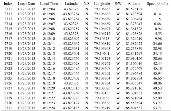
System (GPS) data logger device was used to collect the data needed. The device recorded the positions (including latitudes, longitudes and altitudes) and the instantaneous speeds of the equipped vehicle at 1-second intervals. The records collected by the device were extracted to a personal computer in the form of a spread sheet that shows all the records collected where each record is shown in a separate row in the spreadsheet. Table 1 shows a sample of a spread sheet extracted from the actual data collected. The data were also extracted to a map so that the records can be visualized on the map as a continuous track. The exact locations of right-turning departures from stop positions were identified on the map and therefore the corresponding records were extracted from the spread sheets for analysis. The date and time stamp associated with each record were used to link the map with the spread sheet. As an example, the data shown in Table 1 imply that the subject driver started turning to the right from a stop position (zero speed) at 8:12:04 on October 23, 2013 and reached a speed of 53.712002 km/h at 8:12:24 on the same date, meaning that the driver needed 20 seconds to accelerate from zero to a speed of 53.712002 km/h with the initial and final locations (latitude, longitude and altitude) are as shown on the first and last rows of the table, respectively.
Table 1: Sample spreadsheet created by GPS data logger device
Index Local Date Local Time Latitude N/S Longitude E/W Altitude Speed (km/h) 2711 10/23/2013 8:12:04 43.82378 N 79.106682 W 81.578125 0 2712 10/23/2013 8:12:05 43.823784 N 79.106682 W 81.433594 0.14 2713 10/23/2013 8:12:06 43.823784 N 79.106689 W 81.396484 1.15 2714 10/23/2013 8:12:07 43.82378 N 79.106689 W 81.373047 6.48 2715 10/23/2013 8:12:08 43.823757 N 79.106697 W 81.361328 10.94 2716 10/23/2013 8:12:09 43.82373 N 79.106712 W 81.423828 15.55 2717 10/23/2013 8:12:10 43.823692 N 79.10675 W 81.324219 19.98 2718 10/23/2013 8:12:11 43.823662 N 79.106819 W 81.982422 24.66 2719 10/23/2013 8:12:12 43.823631 N 79.106903 W 82.255859 28.98 2720 10/23/2013 8:12:13 43.823601 N 79.10701 W 82.841797 34.13 2721 10/23/2013 8:12:14 43.823566 N 79.107124 W 83.910156 38.66 2722 10/23/2013 8:12:15 43.823528 N 79.107262 W 84.166016 42.44 2723 10/23/2013 8:12:16 43.823486 N 79.107407 W 84.355469 45.18 2724 10/23/2013 8:12:17 43.823444 N 79.107552 W 84.396484 45.94 2725 10/23/2013 8:12:18 43.823402 N 79.107704 W 84.802734 46.65 2726 10/23/2013 8:12:19 43.82336 N 79.107864 W 84.935547 48.06 2727 10/23/2013 8:12:20 43.823315 N 79.108025 W 85.291016 49.53 2728 10/23/2013 8:12:21 43.823269 N 79.108185 W 85.394531 50.87 2729 10/23/2013 8:12:22 43.823223 N 79.10836 W 85.621094 52.09 2730 10/23/2013 8:12:23 43.823177 N 79.108536 W 85.558594 53.27 2731 10/23/2013 8:12:24 43.823135 N 79.108719 W 85.894531 53.71
Given that the total number of records for one departure is n, the acceleration rate at any second (i) is estimated as the average acceleration rates of previous second (i-1) and successive second (i+1) according to the following equation:
1 1
2
i i ia
v
v
[0 < i < n] (11)Where ai is the estimated acceleration rate at ith second, vi+1 is the instantaneous speed at (i+1)th second,
and vi-1 is the instantaneous speed at (i-1)th second. A total of 266 departures (acceleration profiles) by
12 different drivers and vehicles were included in the analysis. Those profiles include a total of 5319 records (rows). From among those acceleration profiles, 243 profiles (with 4824 records) were used for model development, and the remaining 23 profiles (with 495 records) were reserved for model validation.
3.1. Model development
Based on the data collected for model development, a simple linear regression model for acceleration (using the speed as a predictor variable) was first developed and was found to be inaccurate (with R2 = 0.1452). This inaccuracy may be explained in light of the fact that most subject drivers in the study reported that they accelerate at lower rates during the actual turning maneuver (at the beginning of their departure) and then they apply higher acceleration rates once their vehicles are in line with the cross-traffic stream. This finding is consistent with the findings of a previous research study where Bham and Benekohal (2002) found that acceleration is actually zero at the start of departure and it increases to a maximum value and decreases again to zero at maximum speed. Several other researchers found that the assumption of maximum acceleration at the start of departure (as suggested by the linear acceleration model shown in Equation 5) is unrealistic (see for example Glauz et al. 1980; Akcelik and Biggs 1987; Pitcher 1989). Based on that, the collected data were inspected where it was found that the acceleration rate actually increases at the beginning of the turn until the speed reaches approximately 20 km/h (usually during the initial 4-5 seconds from the start of the departure) and then it starts to decrease. Therefore, two different linear regression models were developed where the first model predicts the acceleration rates for low speeds (less than or equal 20 km/h) and the second model predicts the acceleration rates for speeds higher than 20 km/h. The two models are shown below:
0.5895 0.1273
a
v
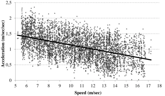
[for speeds lower than or equal 20 km/h; R2 = 0.3272] (12)1.7954 0.066
a v [for speeds higher than 20 km/h; R2 = 0.2397] (13) Where a is the acceleration rate (m/sec2) and v is the speed (m/sec). The two models along with their
respective observed scatter plots are shown in Figure 3 and Figure 4, respectively. The coefficients of the independent variable (speed) in both models were both found to be significantly different from zero at the 95% confidence level. The residuals plots of both models exhibit random dispersion around the horizontal axis, indicating constant variance of errors.
3.2. Model validation
As indicated above, the data set used for validating the regression models include 23 profiles (with 495 records) that were not used to develop the models. The validation statistics for all the models are shown in Table 2. The statistics shown include the mean squared error of validation, MSEv, and the root mean
squared error of validation, RMSEv. As shown in Table 2, the mean squared validation errors for both
models are found to be insignificant. Furthermore, the root mean squared errors of validation, RMSEv,
which indicates that the models are stable and robust when being validated for predictors that were not used in calibrating the models.
Figure 3: Linear acceleration model and scatter plot for observed values (for speeds lower than or equal 20 km/h)
Figure 4: Linear acceleration model and scatter plot for observed values (for speeds higher than 20 km/h)
Table 2: Linear acceleration model
Validation Measure Low Speeds Model High Speeds Model
MSEv 0.103 0.094 RMSEv 0.321 0.307 Se (from calibration) 0.284 0.351 No. of observations 495 495 0 0,5 1 1,5 2 2,5 0 1 2 3 4 5 Acc eler a tio n ( m /s ec /s ec ) Speed (m/sec) 0 0,5 1 1,5 2 2,5 5 6 7 8 9 10 11 12 13 14 15 16 17 18 Acc eler a tio n ( m /s ec /s ec ) Speed (m/sec)
4.
DESIGN TABLE
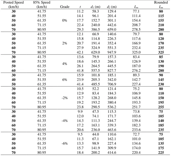
Table 3 was developed to provide different minimum distances, upstream of the intersection, where the proposed pavement markings should extend. Those minimum distances are computed based on different speeds and grades of the cross road (where the departing vehicle is turning into). The length of the design vehicle, Lv, is taken as 6 m, which is the design length of a typical passenger car (TRB 2010). The values for parameters α and β are as given by equations 12 and 13 for low and high speeds, respectively. The calculated distance, Lm, significantly increase with the speed, especially for upgrade roadways. Based on that, distances corresponding to posted speeds that exceed 60 km/h (with 4% upgrade) or 50 km/h (with 6% upgrade) are not included in the table since they are impractically large. It should be noted that the values for Lm shown in Table 3 are more conservative than the typical values for intersection sight distance as provided by the current design guide (AASHTO 2011), which are merely based on the concept of gap acceptance with assumed fixed time gap of 6.5 seconds for a passenger car on a moderate grade.
Table 3: Design table to calculate Lm based on different speeds and grades
Posted Speed (km/h) 85% Speed (km/h) Grade t d1 (m) d2 (m) Lm Rounded Lm 30 41.75 0% 11.2 58.3 129.4 77.1 80 40 51.55 14.1 96.1 201.4 111.4 115 50 61.35 17.7 152.7 301.1 154.4 155 60 71.15 22.4 240.0 442.6 208.7 210 70 80.95 29.3 386.5 659.0 278.5 280 30 41.75 2% 12.1 66.9 140.6 79.7 80 40 51.55 15.8 114.8 226.3 117.6 120 50 61.35 20.7 191.4 352.4 166.9 170 60 71.15 27.9 324.9 551.3 232.4 235 70 80.95 42.1 629.0 947.9 325.0 325 30 41.75 4% 13.6 79.9 157.3 83.4 85 40 51.55 18.6 145.3 266.1 126.9 130 50 61.35 26.1 264.5 445.5 187.0 190 60 71.15 41.8 557.5 827.7 276.2 280 30 41.75 6% 15.9 101.8 185.1 89.3 90 40 51.55 23.9 205.3 342.0 142.7 145 50 61.35 41.4 485.5 706.9 227.4 230 30 41.75 -2% 10.5 52.2 121.4 75.2 80 40 51.55 12.9 83.4 184.3 106.9 110 50 61.35 15.7 128.2 268.0 145.8 150 60 71.15 19.2 193.2 380.4 193.3 195 70 80.95 23.8 290.5 536.2 251.7 255 30 41.75 -4% 9.9 47.5 115.3 73.8 75 40 51.55 12.0 74.1 171.7 103.6 105 50 61.35 14.3 111.3 244.7 139.4 140 60 71.15 17.2 163.1 339.3 182.3 185 70 80.95 20.6 236.0 463.6 233.6 235 30 41.75 -6% 9.5 44.0 110.6 72.7 75 40 51.55 11.3 67.1 162.1 101.0 105 50 61.35 13.3 98.9 227.4 134.6 135 60 71.15 15.7 141.9 309.9 174.0 175 70 80.95 18.4 200.2 414.6 220.4 225
5.
CONCLUSIONS
This paper presented proposed advisory pavement markings that may be painted through a certain distance upstream of an intersection where drivers make unprotected right-turning departures. Those include either signalized intersections where right-turn-on-red (RTOR) is permitted; or unsignalized intersections where a vehicle turns to the right from a controlled minor road into a non-controlled major road. The proposed advisory pavement markings are expected to aid permitted right-turning drivers by setting a limit for them so that the presence of any cross-traffic approaching vehicles over those pavement markings gives an indication to the permitted right-turning driver that a proper time gap is not available to start departure. A methodology is presented to calculate the distance upstream of the intersection where the proposed pavement markings should extend. The presented methodology takes into consideration the speed of the approaching vehicles as well as the acceleration profile of the departing vehicle. A two-stage acceleration profile was established for the departing vehicle based on actual data collected. The collected data suggest that acceleration rate increases with the increase of the speed up to 20 km/h and then it starts to decrease. Based on the parameters associated with the developed acceleration profile models, a design table was provided to aid roadway designers in selecting the distance upstream of the intersection where the proposed pavement markings should be extended. The values given by the design table were found to be more conservative than the typical values for intersection sight distance as provided by the current design guide (AASHTO 2011), which are merely based on the concept of gap acceptance. This finding implies that the time gap suggested by the current design guide, which is 6.5 seconds for a passenger car, may be inadequate for the departing vehicle to accelerate to the same cross-traffic speed if that speed is high.
The pavement markings proposed by this research have the potential to reduce vehicular right-turning crashes. Furthermore, they may ultimately reduce right-turning vehicle-pedestrian crashes as well given that the proposed pavement marking may reduce the driver’s workload so that drivers can pay more attention to pedestrians. However, this assumption is not supported by any direct evidence established by this research. Further research may be needed to investigate this assumption. Also, this research does not propose any configurations (shape, color, or texture) for the proposed pavement markings since those configurations may be established by local transportation authorities in their respective jurisdictions.