Car ownership entry and exit propensities of different generations - a key factor for the development of the total car fleet

ISS/V 0347-6049

. VTISärtryck

161

1991

Car Ownership Entry and Exit Propensities

of Different Generations - A Key Factor for

the Development of the Total Car Fleet

Jan Owen Jansson

Reprint from Developments in Dynamic and Activity-Based

Approaches to Travel Analysis, edited by Peter Jones,

Transport Studies Unit, Oxford University, pp 417 435

w Veg-och Tra k- Statens väg- och trafikinstitut (VT/l . 587 01 Linköping [ St/tillåt Swedish Road and Traffic Research Institute . S-581 01 Linköping Sweden

ISSN 0347-5049

VTI

s_" yck

161

1991

Car Ownership Entry and Exit Propensities

of Different Generations - A Key Factor for

the Development of the Total Car Fleet

Jan Owen Jansson

Reprint from Developments in Dynamic and Activity-Based

Approaches to Travel Analysis, edited by Peter Jones,

Transport Studies Unit, Oxford University, pp 417-435

%]Väg"'OC/I af/k Statensvväg- och trafiiknst/t'ut (VT/) 587 01 Linköping

20 Car Ownership Entry and Exit

Propensities of Different

Generations - A Key Factor

for the Development of the

Total Car Fleet

JAN OWEN JANSSON

1. BACKGROUND AND PURPOSE

Longitudinal cohort analysis, where the cohorts consist of different generations (birth years), proved necessary for explaining the post-war development of car ownership in Sweden. This approach was applied in the forecasting model developed at VTI for the Swedish National Road Administration. The original work was published in Swedish (Jansson et al., (l986)). An English summary

of some of the main characteristics of the model is available in Jansson (1989).

The present paper is a further development of the key relationships of the original model. Some new empirical evidence is drawn upon, which has cast new light

on some issues, but also some doubts on previous contentions.

1.1 Previous Approaches to Car Ownership Modelling

The approach chosen was the result of a preceding literature survey (see Jansson & Shneerson (1983) for details). Three main types of models were identified: (1) Models for predicting the long-terrn development of car ownership based on the notion of "epidemic diffusion". The most refined version of these growth curve models has been worked out at TRRL by John Tanner.

(2) The so-called "stock-adjustment" models, which seek to explain the

short-to medium-run uctuations in purchases of new cars which have a substantial impact on the level of activity of a motorised society.

0.4 _ 0.3 ' Z LL] U 0.2 QC LJJ 0. 0.1 _ 0.0 _{I I I T I I}

10 20 30 40 50 60 70 80 90

AGE

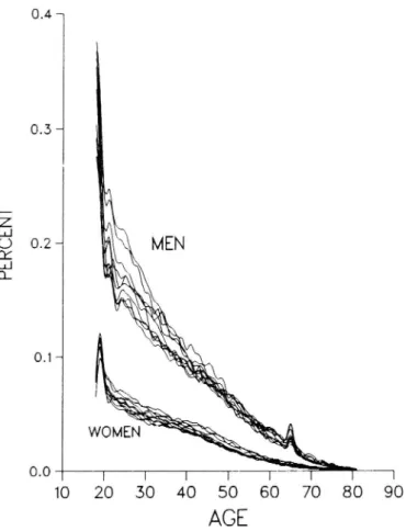
Figure 1a Car ownership entry propensity versus age in percent for men

(3)

and women for ten different years 1975-84

Cross-sectional models based on comparisons of car ownership levels in different regions, cities and parts of cities - and latterly different households. The cross-sectional approach was inspired in the 19705 by discrete choice

analysis, and often as a natural extension of work on modal choice

-a number of c-ar ownership models estim-ated on dis-aggreg-ate (household) data appeared.

0.4 0.3 '-Z Lu U 0.2 cz_Lu 0. 0.1 1 0-0 l 1 1 l l l l ? 10 20 30 40 50 60 70 80 90

AGE

Figure 1b Car ownership exit propensity versus age in percent for men and women for ten different years 1975-84

1.2 The Selected Approach

Through the last approach a deeper knowledge of the socio-economic factors of importance for household car ownership has been obtained. The in uence of local conditions like public transport supply and parking facilities also became more tractable using the disaggregate approach. However, so long as one is relying only on cross-sectional data, the dynamics of car demand including the diffusion process cannot be detected. It was therefore decided that for the Swedish model none of the existing approaches was completely satisfactory; the model was instead calibrated on longitudinal cohort data obtained from the Swedish car register.

Focusing on the car ownership development paths of different generations is

motivated by a belief that the relative "taste" for car ownership is (a) founded

in one s youth and (b) has been rather different for different generations. This does not mean that the usual economic forces of income and price can be assumed to be of no consequence. The main focus of our work has in fact been to modify in the most appropriate way the pure demographic approach to car ownership development, by taking account of the influence of changing incomes and prices in different stages of the life cycle.

In doing this two basic decisions were made. Firstly, it was decided that the

number of entries into car ownership and exits from car ownership ought to

be the object of the study rather than the net level of car ownership. And,

secondly, that since these numbers critically depend on the numbers of carless and car owning persons, respectively, in a particular cohort at a particular time, it was finally decided that the focus should be on the ratio of actual to potential entries, and the ratio of actual to potential exits. The model assumes the "propensity to enter" into car ownership (with its counterpart "exit propensity") to be the primary dependent variable.

The entry propensity is, for each generation, de ned as the ratio of the number of new car owners in a particular year to the total number of carless individuals at the end of the previous year; and the exit propensity is de ned as the ratio of the number of persons who have left car ownership in a particular year to the total number of car owners at the end of the previous year. As can be seen from the diagrams in Figure 1 (which give entry and exit propensities with respect to age for ten different years), both propensities are highly dependent on age for men as well as for women.

This approach to car ownership forecasting is facilitated by viewing the car as an individual rather than a household good. This assumption is supported by the finding that the number of cars per household in Sweden is proportional to the number of adults per household, given the income per adult, age and sex distributions.

The forecasting model is now being further developed in some respects. One shortcoming of the model was the excessive "averaging" involved in the estimation of the entry and exit propensity functions. It was basically assumed that the income elasticity of the entry propensity is the same for every generation (i.e. that the curves of Figure 1a would shift proportionately in response to a general income change). This assumption is, nota bene, much more adequate than assuming the income-elasticity of car ownership to be the same for all generations. However, the accuracy of the predictions of the model could be improved by estimating separately for different age groups both an entry propensity and an exit propensity function of individual income, car price, etc.

This further step has now been taken, and the paper will present the results and discuss their implications for forecasting.

2. THE DETERMINANTS OF CAR OWNERSHIP ENTRY AND EXIT PROPENSITIES

The cohorts studied consist of all Swedes born between 1894 and 1960, and

the observation period is 1975-84. The data sources are basically the car register and inland revenue records, which have been combined to make it possible to follow the car ownership and income development paths of each birth-year cohort through the observation period.

In addition, we have tried to trace the male entry propensity back to 1950, and the female back to 1960. However, here we have had only partial success. It is impossible to trace back the kind of data that are readily available from 1975 onwards; instead, we have resorted to an indirect way of reconstructing the male 1950-1974 series and female 1960-1974 series from the actual car ownership

development, by assuming that:

(a) the exit propensity has stayed constant over time

(b) the shape of the entry propensity with respect to age has stayed constant; only through proportionate shifts of the whole curve have changes in the entry propensity for individual ages occurred.

These are strong assumptions, which are unlikely to be wholly true. Hopefully the resulting reconstruction of the development of the male and female entry propensities has not been seriously biased.

The result of the reconstruction for the average propensities (for all ages) is

shown in Figure 2. As can be seen, the rather irregular pattern for the period

1975-84, for which actual data are available, contrasts with the smooth shape of the reconstructed development before 1975. This is not a real difference,

but a result of the limitations of the calibration procedure.

The main reason why we wanted to go back that far is that we were interested in checking whether the car diffusion process has at any point changed character from vertical to horizontal diffusion. As long as the entry propensity is increasing over and above what economic forces - changes in income, petrol and car prices - explain, a change in "taste for cars" can be assumed to take place. This is vertical diffusion. Horizontal diffusion is de ned to occur after the entry propensity shifting has stopped. However, individuals bring with them their altered preference order as they age, so the sheer population turnover has a diffusion effect as well. The horizontal diffusion process ceases in fact only when a stationary state equilibrium has been obtained. This is further discussed in the next section.

Cor ownership

_{Entry prOpensity}

(%)

_(%)

70 '

Cor ownership

50 *

*

_ 16

20 *

_{* 12}

1950 155 60 56'5m57bmf7rsr' 386384

Figure 2a Male entry propensity and car ownership 1950-84

Cor ownership

Entry propensity

(%)

(%)

15 _ Cor ownership

5

10

A

3

5

_ 2

Entry propensity r. 1

1960 65

70

75

80 84

Yeor

Figure 2b Female entry propensity and car ownership 1960-84 422

We concluded tentatively that vertical diffusion had been important for the development of male entry propensities in the 1950s. As will be clear from

what follows, the statistical analysis of the ten-year period 1975-84 showed no positive contribution of a generation effect (i.e. "lateness" of the birth-year) in explaining male entry propensity. On the contrary, a signi cant negative contribution was detected for young men (18-31 years). For the very youngest women (18-20 years) a significant positive generation effect on entry propensity remained over the period 1975-84. The latter finding is supported by the fact

that the car licence holding of female teenagers has been on the increase in recent times.

2.1 Regression Analysis of the 1975-84 Entry and Exit Propensities As can be seen in Figure la, the entry propensity is a smoothly falling function of age. One single function could be expected to t the data quite well over the whole age range. The exit propensity, on the other hand, has a minimum point around the age of 65 for men, and 60 for women. Two entirely different functions would evidently be applicable on each side of the minimum point. On closer scrutiny the rate of fall of the exit propensity with age, to the left

of the minimum, seems to have a further in ection when people are in their

early thirties, so three different functions should be used in explaining the

relationship between the exit propensity and age. It turned out that the same

is true for the entry propensity. However, the main reason why we have distinguished three age groups in the following regression analysis is that the additional explanatory variables (besides age) have in several cases markedly different effects on the entry and exit propensities of young, middle-aged, and old men and women.

In addition to age we have tested individual income, petrol price, car ownership tax, and chronological time as possible explanatory variables. The observation period is ideal so far as income and petrol price are concerned. For a change, it has not been a period of steady growth in income; total disposable income for households has been stagnant. For different age groups, however, real income has fluctuated a great deal, in particular for the young ones. For example, the mean income for 20 year olds - men as well as women - has varied between a lowest point and a peak, which is about twice as high. The range of income variations in 1975-84 is much narrower for middle-aged and old men (as distinct

from women); the difference between the maximum and minimum for each

particular age is between 10 and 20 per cent. The ownership tax has changed substantially in the period of observation; these changes are a reasonable proxy for the variations in the cost of car ownership per se, since car prices before tax seem to have remained rather stable. Chronological time is a proxy for generation effects; for example, 21 year olds in 1975, 1976 . . . 1984 obviously

represent cohorts of different birth-years. A dummy variable (Dummy 77) appears as well in the exit propensity regressions. It has no economic justi cation, but is there to allow for a suspected flaw in the data for 1977.

In most cases the best t was obtained by an exponential regression equation of the following form:

Entry (exit) propensity = chPyTz exp (aA + bB + $5 + dD) c = constant

I individual real income P petrol price (real)

T car ownership tax (real) A = age

B

S birth-yearSex (1 or O)

D defect dummy for 1977 data (1 or O)

Needless to say, the sex dummy is applicable only when male and female data are merged. The defect dummy was applied only to the exit propensity regressions. A variant of the basic model is obtained by taking the logarithm also of age. That improved the goodness of t somewhat for young men and women so far as the entry propensity is concerned. The resulting elasticities/coef cients

x, y, 2 and a, b, c, (1 of regressions on different age groups are presented in

Tables 1 5.

2.2 Comments on the Results

In all cases, age proved to be by far the most important variable. Age and sex can explain 80-95% of the variations in entry and exit propensities. This was not unexpected in view of the characteristic and regular pattern of the relationships depicted in Figure 1. The question is whether the shifts in the curves that evidently have occurred in the 1975-84 period can be explained by economic factors?

2.2.1 Entry propensity

We started to test just individual income as the independent variable. The explanatory power of income was seemingly quite appreciable - in some instances almost 60%. Further analysis showed that ageing per se might well be the real cause of most of the variations in the entry propensity.

Taking all ages and both sexes together, the main result of the complete model is clearly that the entry propensity falls by S% for every year of age as people are getting older. In the first column of Table l we also see that female entry propensity is, on average, a fraction equal to e 1 of the male entry propensity, everything else remaining the same.

Table 1

Entry Propensity - All Ages

Regression coef cients (with t-values)

Explanatory Both Men Women

variables sexes Income (ln) 0.11 insign 0.25 (6.72) (5.70) Petrol price (ln) -0.52 -0.51 -0.55 (-7.50) (-6.61) (-5.35) Ownership tax (ln) -0.28 -0.10 -0.47 (-7.02) (-2.26) ( 7.95) Age -0.049 -0.044 -0.052 (-99.18) (-70.15) (-76.69) Birth-year 0.009 insign 0.013 (2-98) (2.90) Sex -1.00 (women = 1, men = 0) (-72.69) - --R2(%) 96.6% 95.8% 94.3%

Of the economic variables, the two price proxies are consistently signi cant. The price elasticities have the expected signs, and take values in a relatively narrow range. It is remarkable that income behaves differently. For men, taking all ages, it is insignificant. After dividing the male data into three age groups, this is still true for young men (18-31); for men in their thirties it is just significant, and it is only for the eldest group that the relationship is clear. Is this a true pattern, or just the result of the fact that income and age are strongly correlated up to middle life? For men 18-31 years of age the correlation coef cient of income (ln) versus age equals 0.95. The correlation between income and age for young women is substantially less than for young men, and yet the same pattern of the income elasticity being at its lowest in the lowest age group, and at its highest in the highest age group reappears for women. Disaggregating the data down to sets of ten observations for each particular age, and running the same regressions (except that age is held constant) shows a clear tendency for the income elasticity to grow with age up to about 35 years for men and 45 years for women. With only ten observations estimates are

Table 2

Entry Propensity - Men

Regression coef cients (with t-values)

Explanatory Age Groups

variables 18-31 32-38 39-61 Income (ln) insign 0.76 2.20

(2.89) (12.58) Petrol price (ln) -0.59 -0.41 -0.15

(-8.51) (-5.48) (-2.43)

Ownership tax (ln) -O.33 -O.13 -0.14

(-7.88) (-2.28) (-4.09) Age (ln) -0.33 -0.92 -(-13.05) (-7.99) Age - - -0.049 (-60.14) Birth-year -0.025 insign 0.016 (-8.08) (6.59) _R2(%) 95.2% 84.9% 97.2%

rather uncertain, and cannot be trusted singly, but the overall pattern (see Appendix) is revealing all the same.

2.2.2 Exit propensity

Again age and sex are the completely dominating explanatory variables. Income, on its own, explains nothing of the exit propensity variations for middle aged and old men and women. In the complete model the income elasticity is signi cant with the right sign in the two younger age groups for both men and women; for old men it has the wrong sign, and for women it is insigni cant. In old age the exit propensity is increasingly high for obvious non-economic reasons. However, the car ownership tax level seems to be relatively important for the old. Strangely enough this tax elasticity gets the wrong sign for middle-aged

men, and is rather small for middle-aged women.

Table 3

Entry Propensity - Women Regression coef cients (with t-values) Explanatory Age Groups

variables 18 20 21-37 38-61

Income (ln) 0.25 0.38 1.35

(4.38) (5.60) (20.98) Petrol price (In) -O.88 -0.65 -0.48

(-5.07) (-14.38) (-10.08) Ownership tax (ln) -0.27 -0.59 -0.70 (-2.42) (-18.33) (-22.85) Age (ln) -1.04 -0.36 (-11.18) (-42.01) Age - - -0.064 (-103.11) Birth year 0.033 -0.007 -0.021 (5.77) (-2.55) (-6.44) R2(%) 93.2% 94.2% 98.9%

Breaking down the total data to single years of age, makes the picture quite chaotic (see appendix). Without the steadying in uence of age in the data set, the regression equation explains very little, and few signi cant estimates are obtained. We are bound to conclude that economic forces on the exit propensity are generally weak, and even uncertain as to direction.

3. CONCLUDING REMARKS ON THE DYNAMICS OF CAR OWNERSHIP DEVELOPMENT

Having pointed out some remaining problems and dif culties in explaining entry and exit propensities, it seems appropriate to end by emphasising the insight gained so far, and the advantages of longitudinal cohort analysis as a basis for car ownership forecasting.

Table 4

Exit Propensity - Men

Regression coef cients (with t-values)

Explanatory Age Groups

variables 19-31 32-65 66-78

Income (ln) -O.24 -O.34 0.57*

(-5.09) (-5.30) (2.86) Petrol price (ln) 0.24 -0.18* 0.41 (2.44) (-3.21) (3.39) Ownership tax (ln) 0.17 0.34* 0.51 (2.93) (-lO.84) (7.49) Dummy 77 0.12 0.25 0.15 (3.94) (14.47) (3.98) Age -0.063 -0.035 0.147 (-13.60) (-81.96) (12.09) Birth-year 0.021 0.007 -0.062 (4.84) (2.95) (-6.35) _R2(%) 94.2% 95.5% 95.4% * wrong sign

The main advantages are that the dynamics of car ownership development becomes tractable, and that the old issue of the saturation level seems much less of a problem. In a nutshell, the nature of car ownership dynamics is that we are and will be in practically permanent disequilibrium.

The equilibrium mechanism can be illustrated in the form set out in Figure 3, which shows the number of entries to and exits from car ownership with respect to age. Remember that the total number of entries is the sum of the products of the entry propensity and the number of carless persons of each age. As long as the area between the two curves to the left of their intersection is larger than the area to the right, total car ownership is growing.

Suppose that the entry and exit propensities are frozen in a situation corresponding to that underlying the diagram. That would, of course, not mean that an equilibrium is immediately obtained (i.e. that the two areas on each side of the intersection would suddenly become equal). The two areas will very gradually

develop towards equality, primarily by an expansion of the right-hand area.

Table 5

Exit Propensity - Women Regression coefficients (with t-values) Explanatory Age Groups

variables 19 34 35-59 60-78 Income (ln) -0.15 -0.23 insign

(-6.86) (-4.26)

Petrol price (In) 0.22 0.14 insign (3.67) (3.27) Ownership tax (ln) 0.31 0.19 0.49 (8.92) (7.19) (6.96) Dummy 77 0.06 0.09 0.12 (3.19) (6.68) (3.33) Age -0.060 0.023 0.055 ( 52.80) (-54.70) (10.15) Birth year 0.01 1 0.008 insign

(4.15) (2.89)

P2(%) 96.8% 92.7% 89.2%

This expansion is brought about both by a rising of the exit curve, which in turn is caused by an increase in the number of car owners (and not the exit

propensity, which is assumed to be frozen), and by a fall of the latter part of

the entry curve, which in turn is caused by a decrease in the number of carless

persons moving on into higher ages.

It may well take a whole generation before a stationary state equilibrium obtains. In a simulation illustrated in Jansson et al. (1986) the starting-point

was the Swedish situation in 1975 in respect of population, car ownership, and

entry and exit propensities. Assuming a constant population as well as population

distribution, and constant entry and exit propensities from then on, it was found

that total car ownership would continue to grow until the second half of the next century: all generations which are 18 years or younger in 1975 (including the then unbom ones) will show exactly the same car ownership development paths, while all older generations will show successively (with increasing age as of 1975) lower development paths. Not until all these "older generations" have died off will the stationary state equilibrium appear.

25000 I 22500 20000 J 17500 "

04 1

Figure 3 Number of entries to and exits from car ownership 1984

Saturation is, of course, quite a different state, or rather an extreme case of a stationary state equilibrium. In real life the entry (and possibly also the exit) propensity will continue to change with changing conditions like income, petrol price, car taxes, etc. The question is: for how long will it go on increasing, in response to a growing level of real income? One can image the existence of saturation levels for the entry propensity well below the absolute maximum level of 100%. However, it seems less crucial a matter with this approach than with traditional models of logistic or similar growth curves for car ownership. At present in Sweden the entry propensity is between 2-20% with a sole peak

of about 30% for 18 year old men. The average level of entry propensity for

men has roughly trebled since 1950, and for women since 1965. The next trebling is likely to take very much longer, if it will ever occur. The effect on the level of car ownership of a trebling of current entry propensities will be that the

level for men rises from a good 70% to close to 100%, and the level for women

would be about the same as the present male car ownership level. If and when the entry and exit propensities reach a saturation level, it will take almost another century before car ownership reaches its saturation level, since that is what

it takes for a stationary state equilibrium to appear, given the entry and exit propensities. Well before this imaginary state occurs, I am sure that other aspects of car demand like individual multi-car ownership, quality of service, and car use will prevail over the old issue of cars per adult, let alone per household, which has dominated modelling efforts up to now.

The pertinent point is, however, that we are now so relatively far from the

absolute maximum of the entry propensity that the question of a saturation level

seems premature. A different matter is that a steady increase in the entry propensity will be reflected in a tapering off in the development of the average level of car ownership, as if a saturation level were drawing closer. However, by assuming the entry and exit propensities to be the primary dependent variables, this problem is side-stepped, as it were.

REFERENCES

Jansson J.O. and Shneerson D. (1983) Some approaches to car demand modelling. VTI rapport 251A, Swedish Road and Traf c Research Institute.

Jansson J.O., Cardebring P. and Junghard O. (1986) Personbilsinnehavet i Sverige 1950-2010. VTI rapport 301, Swedish Road and Traf c Research Institute. Jansson J.O. (1989) Car demand modelling and forecasting. A new approach.

APPENDIX - REGRESSION RESULTS FOR EACH SINGLE AGE ENTRY PROPENSITY - MEN

Coefficients (and t-ratio) of log-linear regressions.

b o ) * U D P -* i P r t l .396 .753 .477 Income .53) .76) .25) .48) .16) .64) .16) .55) .97) .19) .47) .72) .46) .56) .52) .19) .83) .02) .28) .97) .10) .45) .88) .90) .53) .31) .53) .87) .87) .64) .99) .87) .13) .61) .04) .76) .12) .00) .32) .30) .54) .99) .22) .24) Petrol price .572 .614 .692 .605 .656 .831 .488 .17) .05) .03) .26) .60) .01) .47) .38) .33) .62) .45) .61) .06) .54) .38) .55) .61) .49) .85) .45) .00) .84) .27) .93) .17) .00) .77) .61) .54) .69) .08) .12) 46) .41) .73) .20) .92) .66) .01) .46) .77) .71) .29) .29) 432 I l l l l l Ownership I H M M b w w w M U N i J W H H A A A A A A A A A A A A A A A A A

APPENDIX (contd) - REGRESSION RESULTS FOR EACH SINGLE AGE

ENTRY PROPENSITY - WOMEN

Coefficients (and t-ratio) of log-linear regressions.

Age Income Petrol price Ownership tax R

18 _ .025 (_ 20) .296 ( .91) .289 ( .97) 0 19 .038 ( 37) _ .020 (_ .08) .071 ( .33) 0 20 .068 ( 56) _ .395 (_1.68) _ .277 (_1.50) 16 21 .230 ( 59) _ .776 ( 1.58) _ .576 (_1.90) 35 22 .307 ( 1.27) .759 (_3.09) _ .478 (_3.58) 62 23 .299 ( 1.18) .708 ( 3.51) _ .440 (_4.08) 68 24 .482 ( 147) _ .658 (_3.07) _ .529 (_4.60) 69 25 .438 ( 177) _ .593 (_3.92) _ .516 (_6.41) 82 26 .682 ( 2 24) .835 ( 4.53) - .637 ( 6.67) 82 27 .189 ( 68) _ .623 (_3.44) _ .559 (_5.90) 78 28 .415 ( 1 76) _ .850 ( 5.23) _ .630 ( 7.39) 85 29 .238 ( 80) _ 682 ( 3.07} _ .483 (_4.16) 62 30 .144 ( 65) _ .733 (_4.23) .545 (_6.05) 80 31 _ .066 (_ 25) _ .755 (_3.61) _ .585 (_5.55) 79 32 _ .090 (_ 27) .636 ( 2 51) _ .500 (_3.95) 64 33 .124 ( 39) _ .796 (_3 33) _ .539 (_4.48) 69 34 .207 ( 81) _ .630 (_2.92) _ .467 (_4.16) 62 35 .147 ( .80) _ .662 (_3.88) _ .510 ( 5.63) 77 36 .198 ( 1.11) _ .624 (_3.81) _ .482 (_5.64) 77 37 .257 ( 1.07) _ .419 (_1.93) _ .389 (_3.64) 55 38 .342 ( 2.86) _ .579 (_5.33) _ .491 (_9.43) 91 39 .440 ( 1.68) _ .605 ( 2.59) _ .524 (_4.64) 69 40 .754 ( 6.01) _ .652 (_5.83) _ .499 (_8.95) 92 41 .556 ( 2.53) _ .592 ( 2.97) _ .555 (_5.38) 78 42 .619 ( 2.50) .571 (_2.66) _ .566 (_5.11) 77 43 .637 ( 2.54) _ .600 ( 2.88) _ .615 (_5.87) 81 44 .835 ( 2.55) .417 (_1.57) _ .483 (_3.64) 71 45 1.144 ( 5.92) _ .607 (_3.86) _ .624 (-7.78) 92 46 1.081 ( 4.64) _ .559 ( 2.78) _ .541 ( 5.09) 85 47 .910 ( 2.37) _ .401 (_1.20) _ .558 (_3.20) 67 48 1.060 ( 4.86) _ .364 (_1.85) _ .489 (_4.81) 88 49 .866 ( 3.50) _ .591 ( 2.62) _ .648 (_5.63) 84 50 1.062 ( 4.97) .504 ( 2.58) .549 ( 5.92) 89 51 1.151 ( 3.92) _ .718 (_2.61) _ .620 (_4.43) 80 52 1.020 ( 5.41) _ .750 (_4.10) _ .595 (_6.36) 89 53 1.024 ( 4.90) _ .510 ( 2.40) _ .496 (_4.56) 86 54 .860 ( 3.26) .532 ( 1.98) _ .520 ( 3.83) 76 55 1.079 ( 4.31) _ .449 ( 1.79) _ .492 (_3.95) 85 56 .640 ( 2.33) .250 ( .91) .533 ( 3.91) 79 57 .799 ( 3.87) _ .224 (_1 13) _ .573 (_5.80) 91 58 .600 ( 2.10) .326 (_1.14) _ .503 (_3.43) 72 59 .855 ( 5.97) _ .499 (_3.13) _ .474 (_5.70) 91 60 .484 ( 3.35) .123 ( .71) _ .501 ( 5.59) 90 61 .688 ( 2.18) .124 ( .32) .354 (_1.84) 73

APPENDIX (contd) - REGRESSION RESULTS FOR EACH SINGLE AGE

EXIT PROPENSITY - MEN

Coefficients (and t-ratio) of log-linear regressions.

2

Age Income Petrol price Dummy 77 Time R

18 1.292 ( 7.55) .809 ( 1.11) .009 ( .04) .054 ( .39) 88 19 .105 ( 1.75) .209 ( 1.55) .064 ( .73) .136 ( 3.50) 84 20 .210 ( 1.52) .435 ( 1.60) .005 ( .07) .116 ( 2.36) 25 21 .163 ( .29) .423 ( 1.15) .146 ( 1.32) .024 ( .40) 12 22 .089 ( .60) - .060 (- .36) .113 ( 2.17) .132 ( 4.64) 82 23 .142 ( .62) _ .161( .77) .051. ( .82) .148 ( 4.12) 74 24 .153 ( .41) _ .004 ( .02) .105 ( 1.85) .113 ( 3.46) 74 25 .139 ( .30) .053 ( .23) .124 ( 1.96) .121 ( 3.40) 73 26 .036 ( .10) .068 ( .39) .138 ( 2.79) .136 ( 4.99) 86 27 .382 ( .89) .034 ( .17) .164 ( 2.90) .100 ( 3.19) 77 28 .697 ( 1.67) .093 ( .48) .171 ( 3.20) .077 ( 2.55) 80 29 .802 ( 1.37) .255 ( .92) .200 ( 2.76) .050 ( 1.21) 71 30 1.616 ( 2.38) .374 ( 1.14) .152 ( 1.87) .060 ( 1.28) 61 31 1.376 ( 2.21) .065 ( .21) .190 ( 2.55) .015 ( .33) 63 32 1.473 ( 2.51) _ .019 ( .07) .183 ( 2.47) .033 ( .73) 54 33 1.365 ( 2.77) .179 ( .74) .149 ( 2.38) .008 ( .20) 64 34 .937 ( 1.13) .117 ( .27) .205 ( 1.84) .030 ( .46) 18 35 1.559 ( 2.05) .246 ( .64) .214 ( 2.29) .009 ( .17) 40 36 1.482 ( 1.99) .265 ( .72) .189 ( 2.10) .025 ( .49) 40 37 -2.380 ( 3.23) .380 ( 1.13) .176 ( 2.01) .026 ( .52) 61 38 1.531 ( 1.77) .132 ( .40) .154 ( 1.71) .034 ( .66) 35 39 1.878 ( 1.50) .060 ( .15) .204 ( 2.06) .047 ( .84) 43 40 1.668 ( 1.06) .256 ( .47) .144 ( 1.18) .065 ( .95) 6 41 2.307 ( 1.52) .400 ( .75) .097 ( .94) .080 ( 1.33) 26 42 4.027 ( 3.34) .809 ( 1.94) .082 ( 1.04) .086 ( 1.91) 64 43 2.777 ( 2.16) _ .482 ( 1.10) .082 ( .84) .039 ( .72) 26 44 3.220 ( 2.05) .270 ( .55) .148 ( 1.23) .047 ( .69) 37 45 2.531 ( 1.65) .089 ( .20) .232 ( 2.24) .050 ( .87) 47 46 2.324 ( 1.24) .408 ( .72) .159 ( 1.50) .089 ( 1.42) 24 47 -2.063 ( 1.23) .406 ( .77) .168 ( 1.77) .089 ( 1.59) 36 48 4.068 ( 2.45) ~ .851 ( 1.59) .086 ( 282) .093 ( 1.54) 41 49 3.214 (-1.96) .399 ( .83) .153 ( 1.52) .048 ( .84) 36 50 - 2.745 (- 1.14) .229 ( .33) .169 ( 1.20) .048 ( .61) 8 51 -2.015 ( .83) .200 ( .29) .144 ( 1.05) .042 ( .53) O 52 .709 (- .31) .170 ( .26) .231 ( 1.78) .034 ( .45) 4 53 2.556 (_ .86) .296 ( .32) .177 ( 1.12) .044 ( .43) 0 54 2.021 (-1.28) .462 ( .95) .167 ( 1.73) .072 ( 1.31) 31 55 2.281 ( 1.33) .325 ( .65) .204 ( 1.86) .024 ( .39) 27 56 3.547 ( 1.62) .664 (-1.28) .128 ( 1.16) .035 ( .57) 12 57 -1.630 (_ .74) .085 ( .16) .124 ( 1.10) .007 ( .11) 0 58 2.214 ( 1.42) .400 ( .87) .176 ( 1.79) .014 (_ .24) 27 59 2.374 ( 2.68) .178 ( .62) .266 ( 5.14) .044 ( 1.11) 76 60 .409 ( .43) .178 ( .56) .180 ( 3.44) .039 ( .81) 65 61 1.554 (-1.95) .480 ( 1.93) .016.( .29) .056 ( 1.29) 37

434

APPENDIX (contd) - REGRESSION RESULTS FOR EACH SINGLE AGE EXIT PROPENSITY - WOMEN

Coefficients (and t-ratio) of log-linear regressions.

Age 18 .443 19 .102 20 .114 21 .229 22 .054 23 .197 24 .030 25 .281 26 .030 27 .132 28 .887 29 1.705 30 1.779 31 .471 32 .002 33 .574 34 .200 35 .605 36 3.456 37 - .873 38 .052 39 2.735 40 1.084 41 2.130 42 .660 43 1.579 44 1.613 45 3.632 46 .198 47 1.088 48 .289 49 .005 50 4.154 51 3.487 52 .401 53 .200 54 1.578 55 .125 56 1.985 57 .598 58 .653 59 .101 60 .364 61 .507 Income .971 .851 .486 .183 .319 .040 .147 .055 .106 .235 .009 .117 .067 .087 .062 .010 .037 .022 .155 .138 .086 .210 .349 .130 .072 .234 .106 .096 .209 .139 .178 .058 .037 .054 .034 .243 .141 .071 .267 .276 .312 .096 .504 .333 5. 2. 2. Petrol price 55) 1.7) 12) .35) .68) .15) .01) .50) .64) .15) .05) .49) .31) .29) .39) .61) .11) .12) .73) .96) .55) .67) .94) .65) .49) .20) .40) .31) .71) .51) .81) .19) .10) .29) .16) .77) .88) .25) .03) .98) .04) .22) .46) .22) Ownership tax .634 .525 .283 .111 .190 .207 .241 .207 .152 .273 .195 .414 .415 .185 .306 .209 .243 .120 .540 .230 .162 .465 .080 .290 .085 .305 .110 .342 .080 .226 .105 .095 .177 .197 .060 .262 .273 .177 .075 .217 .296 .225 .347 .326 r n x b A A A A A A A A A A Å A A A A A A Å A A Å A / N A A A A A A A Å A A A A A A / N A Å A A A A H M N U J N I l b J D I N H N b H r H N ,.. -H O H M L a J P -U H .69) .84) .77) .26) .96) .70) .85) .24) .02) .91) .80) .69) .03) .91) .94) .01) .17) .74) .18) .91) .36) .86) .61) .29) .77) .99) .56) .49) .49) .12) .40) .44) .56) .91) .51) .58) .86) .18) .56) .40) .36) .20) .52) .18) .128 .033 .028 .079 .105 .017 .051 .048 .083 .120 .026 .015 .031 .096 .055 .091 .135 .096 .036 .123 .120 .044 .096 .115 .080 .033 .061 .004 .091 .046 .109 .096 .014 .014 .115 .094 .116 .026 .126 .032 .024 .032 .068 .301 Dummy 77 < 3.54) .41) .61) .70) .11) .18) .05) .42) .53) .59) .45) .19) .38) .81) .94) .57) .31) .65) .32) .05) .56) .48) .42) .80) .48) .41) .66) .04) .09) .44) .79) .88) .10) .23) A | M H P l H N N r lr w-J k P h) I N H F * b i l .69) H.53) .37) .86) .33) .12) .64) A A A A A A A A A A A A A A A A A A A A A A A A A A A A A A A A A A A A A A A A A A N H .70) _ .89) _ .25) Time .486 .084 .057 .089 .051 .067 .044 .023 .007 .013 .117 .179 .211 .091 .033 .079 .024 .060 .482 .121 .008 .361 .127 .299 .080 .196 .193 .480 .014 .201 .047 .069 .590 .509 .018 .078 .269 .004 .344 .159 .105 .052 .015 .142 r w u r .29) .78) .38) .26) .85) .58) .85) .54) .08) .09) .93) .78) .28) .36) .23) .55) .10) .30) .94) .27) .07) .24) .35) .55) .43) .02) .80) .21) .05) .75) .41) .22) .01) .26) .08) _ .17) .60) .01) .35) .63) .13) .11) .09) .62)