Volatility Forecasting on the Stockholm Stock Exchange

Volatility Forecasting on the

Stockholm Stock Exchange

Paper within: Civilekonom examensarbete/Master thesis in Business Administration (30hp), Finance track

Authors: Gustafsson, Robert

Quinones, Andres

Master’s Thesis in Business Administration/Finance

Title: Volatility Forecasting on the Stockholm Stock Exchange Authors: Robert Gustafsson & Andres Quinones

Tutors: Andreas Stephan & Jan Weiss

Date: 2014-05

Subject terms: Implied Volatility, Volatility Forecasting, Time-Series analysis.

Abstract

The aim of this thesis is to examine if the implied volatility of OMXS30 index options represented by the SIX volatility index can produce accurate and unbiased forecasts of the future volatility on the Stockholm Stock Exchange. In addition we also examine if the implied volatility contains any additional information about the future volatility that cannot be captured by various time-series forecasting models. The forecasts made by the SIX volatility index and the time-series models are evaluated by their accuracy, predictive power and informational content. Lastly GMM-estimations are performed to test whether implied volatility contains any incremental information. By analyzing our results we find that the SIX volatility index is a good predictor of the future realized volatility on the OMXS30, however the results also indicate a bias in the forecasts. The

GMM-estimations indicates that the SIX volatility index contains no additional

Table of Contents

1 Introduction ... 1

2 Theoretical Background ... 6

2.1 Different Types of Volatility ... 6

2.1.1 Historical Volatility ... 6

2.1.2 Realized Volatility ... 6

2.1.3 Implied Volatility & Black-Scholes ... 7

2.2 Characteristics of Volatility ... 8

2.2.1 Volatility Clustering ... 9

2.2.2 Asymmetric Responses to Shocks ... 9

2.2.3 Persistence of Volatility ... 10

2.2.4 Volatility Smile ... 10

2.2.5 Implied Distribution ... 11

3 Method: ... 13

3.1 Forecasting Using Models ... 13

3.1.1 Forecasting Principle ... 13

3.1.2 Naïve Historical Model ... 14

3.1.3 Autoregressive Moving Average (ARMA) ... 15

3.1.4 Choice of ARMA Models ... 17

3.1.5 Forecasting with ARMA (2,1) ... 18

3.1.6 Forecasting with ARIMA (1,1,1) ... 19

3.2 Autoregressive Conditional Heteroskedastic (ARCH) Models ... 19

3.2.1 ARCH Model ... 19

3.2.2 GARCH Model ... 20

3.2.3 EGARCH Model ... 21

3.2.4 Choice of ARCH Models ... 22

3.2.5 EGARCH Model Estimation Using Maximum Likelihood ... 22

3.3 Quality Evaluation of Forecasts ... 23

3.3.1 Root Mean Square Error ... 23

3.3.2 Mean Absolute Error ... 24

3.3.3 Mean Absolute Percentage Error ... 24

3.3.4 Theil Inequality Coefficient ... 25

3.3.5 Predictive Power ... 25

3.3.6 Informational Content ... 26

3.4 Additional Information in Implied Volatility ... 27

4 Data ... 29

4.1 General Data Description ... 29

4.3 SIXVX as a Measure of Implied Volatility ... 29

4.4 Graphs and Descriptive Statistics ... 30

5 Results ... 34

5.1 Data and Descriptive Statistics in the Rolling Estimation Period ... 34

5.2 Estimation of Model Parameters ... 36

5.3 Descriptive Statistics of Forecasts ... 40

5.4 Forecast Evaluation ... 41

5.5 Predictive Power ... 41

5.6 Informational Content ... 43

5.7 Additional Information in SIXVX ... 44

6 Conclusion ... 47

6.1 General ... 47

6.2 Relative Performance of the Forecasting Methods ... 47

6.3 Biasedness of the Forecasts ... 48

6.4 Additional Information in Implied Volatility ... 48

6.5 Final Remarks ... 49

Figures

Figure 1: Volatility Smile ... 11

Figure 2: Implied Distribution ... 12

Figure 3: Forecasting Methodology ... 14

Figure 4: Comparison of OMXS30 and SIXVX ... 31

Figure 5: Daily return series of OMXS30 ... 31

Figure 6: Daily computed volatility of the OMXS30 ... 32

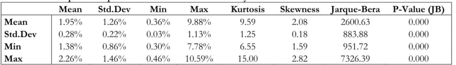
Figure 7: Distribution and descriptive statistics of the daily-realized volatility ... 32

Figure 8: The 22-day ahead average realized volatility over the whole sample period 33 Figure 9: Distribution and descriptive statistics of the 22-day ahead average realized volatility over the whole sample period. ... 33

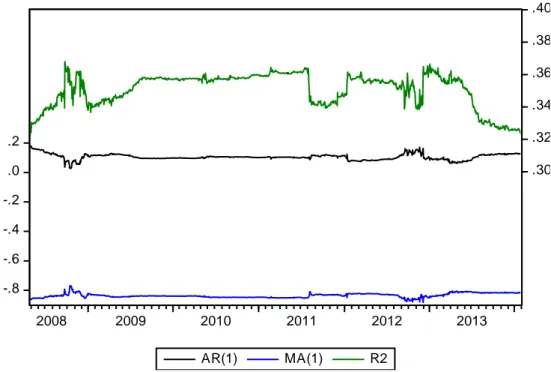
Figure 10: Estimated ARMA (2,1) parameters ... 37

Figure 11: Estimated ARIMA (1,1,1) parameters ... 38

Figure 12: Estimated EGARCH parameters ... 39

Tables

Table 2: Autocorrelation of Realized Volatility ... 35

Table 3: Augmented Dickey-Fuller Unit Root Test ... 35

Table 4: ARMA(2.1) Model Estimation ... 37

Table 5: ARIMA(1.1.1) Model Estimation ... 38

Table 6: EGARCH Model Estimation ... 39

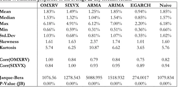
Table 7: Statistical properties of the average 22-day forecast results ... 40

Table 8: Forecast Performance Measure ... 41

Table 9: Predictive Power ... 42

Table 10: Information Content ... 44

Table 11: GMM estimations OMXRV ... 46

Appendices

Appendix 2: Histograms of Forecasts ... 55

Introduction

1 Introduction

In this part we will present the background to the area of volatility and review some of the previous research on the topic of volatility forecasting. We will also highlight the problem statement, purpose and limitations of our thesis.

1.1 Background

In recent years much of the financial research has been aimed at studying volatility modeling. This is due to the fact that volatility is the most common determinant of risk in the financial markets. Volatility is a measure of deviation from the mean value and high volatility means high risk (Figlewski 1997). Volatility is often used as input in asset pricing models such as the Capital Asset Pricing Model and is also important in the pricing of various derivatives.

The options market grew heavily after Black & Scholes (1973) introduced a new method of pricing options. The Black-Scholes model provided investors with a simplified way for the pricing of European options. The inputs for applying the model are all easily observable except one which is the volatility of the options underlying asset. Since volatility is unobservable it has to be estimated and it is not straightforward how to do that. But the crucial role of volatility in the financial markets makes it important that reliable future estimates can be constructed.

Much research has been focused on how to estimate future volatility and many different ways of forecasting has been developed. Model based forecasting such as Autoregressive Conditional Heteroskedasticity (ARCH) models are a common forecasting technique but the use of implied volatility is also widely researched.

Implied volatility draws on the relationship between the price of an option and the volatility of the underlying asset that the Black-Scholes model implies. Since the volatility is the only unobservable input in the pricing of options it is possible to go backwards through the formula to retrieve the volatility from the option price. Implied volatility is therefore believed to be the markets future assessment of the volatility (Hull 2012). The belief is that implied volatility may possibly contain more information about future volatility than what might be contained by forecasting models that are based on historical data (Knight & Satchell 1998).

Introduction

1.2 Previous Research

How to estimate future volatility has been a very hot topic of research for quite some time. Many papers regarding both models based forecasting and forecasting using implied volatility has been published.

The earlier studies of Latane & Rendelman (1976), Chiras & Manaster (1978) and Beckers (1981) all came to the conclusion that implied volatility did have informational content on future volatility. However the authors at this time did not have access to relevant time series data so these papers focused more on cross-sectional tests with a certain sample of stocks.

Regarding research on the forecasting performance provided by different forecasting models the paper of Akgiray (1989) achieves results that are indicating that forecasting with a GARCH model outperforms historical volatility and the Exponential Weighting Moving Average (EWMA) Model. Andersen & Bollerslev (1998) also reach the same conclusion that the GARCH model performs relatively well with their model explaining around 50 % of the informational content of future volatility. Cumby et al. (1993) researches the out of sample forecasting ability of an Exponential GARCH model (EGARCH). They reach the conclusion that the EGARCH outperforms the forecasting ability of historical volatility but that the overall explanatory power is not excellent. Different types of ARMA-models can also be used to forecast volatility. The research of Pong et al. (2004) concludes that an ARMA (2,1) model can be useful when forecasting volatility over shorter time horizons.

Regarding papers concerning implied volatility where extensive time-series data has been used Canina & Figlewski (1993) investigated the predictive power of implied volatility derived from options on the S&P 100 index. Their results showed that implied volatility was a poor forecast of realized volatility. Contrarily the study of Lamoureux & Lastrapes (1993) finds that implied volatility were in fact a good predictor of realized volatility and outperformed model based forecasting. Their study focused on 10 stocks with options traded on the Chicago Board of Option Exchange (CBOE). Day & Lewis (1992) examines implied volatility from options on S&P 100 and concludes that implied volatility has significant forecasting power. Although their research also concludes that implied volatility necessarily does not contain more information than models such as GARCH/EGARCH. Fleming (1998) also examines if implied volatility from S&P 100

Introduction

options is an efficient forecasting technique. In contrast to Day & Lewis (1992) Fleming (1998) concludes that implied volatility in addition to outperforming historical volatility also outperforms ARCH type models.

Most recent studies focus on the informational content of so called volatility indices. Blair et al. (2001) investigate the explanatory power of the S&P 100 volatility index (VXO), which is an index of implied volatility on the S&P 100. Blair reaches the same conclusion as the articles of Lamoureux & Lastrapes (1993) and Fleming (1998) that the implied volatility performs better than model based forecasting. A similar study performed by Becker et al. (2006) on the S&P 500 volatility index (VIX) shows a positive correlation between the VIX and future volatility. Their research does not contradict that implied volatility can be a better forecaster than using time series models. A year later in 2007 Becker et al. published a follow up on their initial research and investigate whether implied volatility contains any additional information that is not covered by any model-based forecasts. Their results indicate that implied volatility does not contain any additional information of the future volatility.

However even if implied volatility is found to be the best forecaster in many papers it does tend to produce biased forecast. Both Lamoureux & Lastrapes (1993) and Blair et al. (2001) find evidence of a downward bias, hence implied volatility underestimates the future volatility. Fleming (1998) also detects that the forecast made by the implied volatility might be biased.

The Meta-analysis of Granger & Poon (2003) looks at a total of 93 articles concerning volatility forecasting. They find that the forecasting models that perform the best are the models that take the asymmetry of volatility in account such as an EGARCH or GJR-GARCH model. But they also conclude that implied volatility outperforms forecasting models in general. To them the question is not whether volatility is possible to forecast or not, it is how far in the future we can accurately forecast it. EGARCH and GJR-GARCH are asymmetric models that were developed by Nelson (1991) and Glosten et al. (1993) respectively.

Introduction

1.3 Problem Description

As mentioned in section 1.1 volatility plays a big role in financial markets. Volatility is used in decision-making processes and risk management but is also important in derivative pricing. Hence it is imperative that reliable future estimates can be produced. This thesis will be aimed at comparing different volatility forecasting methods on the Stockholm Stock Exchange. Our main focus will be on implied volatility that is represented by an index called SIX Volatility index (SIXVX) and how well future volatility can be forecasted in the Swedish market. We want to examine and evaluate which forecasting method that produces the better forecasts of the future realized volatility.

Most of the previous research in the area is performed for the US market. The results of these studies are not unanimously but there is more weight on research articles that conclude that implied volatility is the best predictor. Due to the lack of studies on implied volatility on the Swedish market the authors of this thesis see an opportunity in potentially providing valuable insights on the topic of volatility forecasting. To accomplish this task we will focus on the OMX Stockholm 30 index and test the forecasting ability of its volatility index (SIXVX) on future realized volatility. Furthermore since most previous research concludes that implied volatility is the best predictor of future volatility we want to put our main focus on implied volatility. The outcome that implied volatility is the best is usually obtained by comparing the forecast results from each model-based forecast and the implied volatility. What is not often investigated is if implied volatility can outperform a combination of model-based forecasts as studied in Becker et al. (2007).

More specifically these are the questions that we want to answer:

 Does implied volatility produce a better forecast of the future realized volatility than what is produced by forecasting using time-series models?

 Does implied volatility produce an unbiased forecast of the future realized volatility?

 Does implied volatility contain any additional information about the future realized volatility that is not captured by the model-based forecasts?

Introduction

1.4 Purpose

The purpose of this thesis is to determine if implied volatility is a good method to use when forecasting the volatility on the Stockholm stock exchange. More specifically we want to examine if implied volatility produces an unbiased and better out-of-sample forecast of the realized volatility on the Stockholm stock exchange than model-based forecasts. To fulfill our purpose and provide answers to our research questions we will evaluate the forecasting accuracy, predictive power and informational content of each forecasting technique. We will also investigate if implied volatility contains any additional info than what is captured by a combination of the various time-series models.

1.5 Delimitations

The data used for the thesis consists of roughly 10 years of daily data since the volatility index has only existed since 2004. There is no possibility to cover all the forecasting models that exists so we have limited ourselves to those that fit the characteristics of our data. The same goes for the quality evaluation methods that are used to compare the forecasting accuracy of the different forecasting methods. OMX Stockholm 30 Index will be used as the representative for the entire Swedish equity market.

1.6 Thesis Outline

Here we will present a brief overview of the overall outline of the thesis. Chapter 1 has introduced the reader to the subject of volatility, previous research, and our purpose and research questions. Chapter 2 will continue to explain what volatility is, the different types of it and the characteristics that are observable in volatility. These characteristics are the foundation for the 3rd chapter where we will describe our chosen forecasting methods and how we will forecast using these methods. In the same chapter we will also go over how the forecasts will be evaluated and the different tests that we will conduct such as predictive power, informational content and the test for additional information. Chapter 4 is a chapter about the data used in the thesis. The chapter will explain how the SIX volatility index of implied volatility is composed and how it can be used to forecast with. Some basic descriptive statistics will also be examined. In chapter 5 the different results from the forecasting accuracy and the different tests mentioned in chapter 3 will be presented. To finalize our thesis there will be a chapter concerning our conclusions and suggestions for future research that could be conducted.

Theory

2 Theoretical Background

In this chapter of the thesis we intend to give the readers an overview of the theoretical background to the concepts of volatility, implied volatility and its common features.

2.1 Different Types of Volatility

2.1.1 Historical Volatility

Volatility has many different meanings in the financial world, the most usual is the historical volatility. The historical volatility is usually denominated as the standard deviation of previously observed daily returns. The volatility is used as a measure of risk of the underlying asset, usually a stock. The standard deviation of a sample 𝜎̂ is calculated using the following formula, where rt is the observed return and 𝑟 is the mean

return. 𝜎̂ = √ 1 𝑛 − 1∑(𝑟𝑡− 𝑟 𝑛 𝑡=1 )2 ₍₁₎

The returns between the price P at time t and the price in the previous period are continuously compounded, which implies

𝑟𝑡 = ln ( 𝑃_𝑡

𝑃𝑡−1). (2)

2.1.2 Realized Volatility

When evaluating different forecasting methods it is important to have a good measure of the ex post volatility to evaluate the forecasts against. Since historical volatility is usually computed using daily closing prices a lot of the information is lost (Andersen & Benzoni 2008). Therefore another way of computing the ex post volatility is to estimate the so-called realized volatility. When estimating the historical volatility daily data or less-frequent data is often used, while realized volatility is estimated using intraday data (Gregoriou 2008). The usual way to compute realized volatility is to take the square root of the sum of the squared intraday returns to get the daily volatility. But it is also possible to use the daily range of the high and low prices to catch the intraday movements (Martens & Van Dijk 2007). The realized volatility is calculated to

Theory

represent the true out of sample volatility and for the OMX Stockholm 30 index it will be calculated in the following way.

𝑅𝑉𝑡 = ln (

𝑂𝑀𝑋𝑆30_{ℎ𝑖𝑔ℎ,𝑡}

𝑂𝑀𝑋𝑆30𝑙𝑜𝑤,𝑡) (3) Where 𝑂𝑀𝑋𝑆30_{ℎ𝑖𝑔ℎ,𝑡} stands for the highest intraday price of the OMXS30 on that particular day and 𝑂𝑀𝑋𝑆30_{𝑙𝑜𝑤,𝑡} is the lowest intraday price on the same day. RVt is

then a proxy for the realized daily volatility on day t.

The reason for applying a based estimate for realized volatility is that a range-based estimation catches more of the intraday movements of the volatility than the method of using the closing prices (Alizadeh 2002). Andersen et al. (2003) recommends that observations should be collected within 5-minute intervals of the squared intraday returns in order to compute the realized volatility. But without access to costly intraday data range-based calculations are preferred. Parkinson (1980) conclude that a logged daily high-low price range is an unbiased estimator of the daily volatility that is five times more efficient than computing daily volatility using only the closing prices.

2.1.3 Implied Volatility & Black-Scholes

The Black-Scholes option-pricing model is the result from the pioneering article by Black & Scholes (1973). The model revolutionized the way for traders on how to hedge and price derivatives. To determine the price of a European call or put option only a few inputs are needed. These inputs are the risk free rate, time to maturity, stock price, strike price and the volatility. As we mentioned in section 1.1 the only unobservable input is the volatility. However for the pricing formula to work a number of assumptions has to be made.

1. Lognormally distributed returns, which means that the returns on the underlying stocks are normally distributed.

2. No dividends are paid out on the stocks.

3. Markets are efficient so future market movements cannot consistently be predicted. Hence stock prices are assumed to follow a geometric Brownian motion with a constant drift and volatility. Denoting St as the stock price at time

t, μ as the drift parameter, σ as volatility and Wt as the Brownian motion, the

Theory

dSt = μStdt + σStdWt . (4) The formula of a geometric Brownian motion is then used to calculate the Black-Scholes differential equation. The solution to the differential equation is the actual pricing formula. Let S0 denote the initial stock price at the start of the options maturity,

r the risk free rate, K the denotation for the strike price of the option and T the maturity

of the option. The pricing equation can be written as:

Pricing equation for a call option: 𝑐 = 𝑆₀𝑁(𝑑₁)– 𝐾𝑒−𝑟𝑇_𝑁(𝑑

2) (5) Pricing equation for a put option: 𝑝 = 𝐾𝑒−𝑟𝑇_𝑁(−𝑑

2) − 𝑆0𝑁(−𝑑1) (6) N(dx) is the function for the cumulative probability distribution function for a standardized normal distribution and is expressed in the following way where σ is the volatility. 𝑑₁ = 𝑙𝑛 ( 𝑆0 𝐾 ) + (𝑟 + 𝜎 2 2 ) 𝑇 𝜎√𝑇 (7) 𝑑₂ = 𝑙𝑛 ( 𝑆₀ 𝐾 ) + (𝑟 − 𝜎 2 2 ) 𝑇 𝜎√𝑇 = 𝑑1− 𝜎√𝑇 (8)

Implied volatility can then be calculated by rearranging the Black-Scholes pricing formula to extract the volatility from observed option prices. While historical volatility is only based on past movements of an asset it is not an optimal measure for forecasting since we then want to look into the future. Implied volatility is a more forward-looking measure that can be seen as what the market implies about the future volatility of an asset (Hull 2012).

2.2 Characteristics of Volatility

Granger & Poon (2003) point out that volatility has many characteristics that have been empirically observed and which all can have an effect when forecasting future volatility. Since the purpose of our thesis is to model and analyze different methods of volatility forecasting certain features and common characteristics that are typical for volatility needs to be identified. To get reliable future estimates it is important that we implement forecasting methods that take these characteristics of volatility into consideration.

Theory

Therefore before we choose which models to apply we want to point out these common features of financial market volatility mentioned by Granger & Poon (2003). These characteristics are: volatility clustering, leptokurtosis, persistence of volatility and asymmetric responses from negative/positive price shocks.

2.2.1 Volatility Clustering

Volatility clustering is a phenomenon that describes the tendency for large (low) returns in absolute value to be followed by large (low) returns. Hence one can argue that volatility is not constant over time but instead tends to vary over time and this is something that is observed empirically. Mandelbrot (1963) was the first to describe this pattern and it can be found in most financial return series. One explanation for this observed phenomenon is according to Brooks (2008) that information that affects the return of an asset does not come at an evenly spaced interval but it rather occurs in clusters. This is very logical since one would expect that stock returns would be more volatile if new information about the firm, their business field and their competitors arrives and this is usually available for investors when firms release their financial reports. It is likely that our return series will experience volatility clustering and therefore it is important to use volatility models that take this characteristic into account. We will return to this in section 3.2.1 when discussing ARCH type models.

2.2.2 Asymmetric Responses to Shocks

Another common empirically observable feature for the volatility of stock returns mentioned by Brooks (2008) is its tendency for it to increase more following a negative shock than a positive shock of the same magnitude. In other words this means that past returns and volatility are negatively correlated. This is also known as the leverage effect if equity returns are considered and was first found by Black (1976) and is linked to the hypothesis that negative shocks to stock returns will increase its debt-to equity ratio. Hence it will increase the risk of default if the price of a stock falls. Christie (1982) is another paper regarding the leverage effect, with the conclusion that volatility is an increasing function of a firm’s level of leverage. Therefore volatility is more affected by a negative shock than a positive shock. Brooks (2008) acknowledges another explanation for asymmetric responses to shocks that is the volatility feedback hypothesis. The volatility feedback hypothesis is according to Bekaert et al. (2000) linked to time-varying risk premiums. This means that if volatility is being priced then

Theory

an increase in volatility would require higher expected returns in order to compensate for the additional risk and as a consequence of this the stock price would decline immediately. Hence the causality of these two hypotheses is opposite each other. While it is hard to determine exactly why this asymmetry exists we will still examine if it is present in our dataset, if so an asymmetric GARCH model could be preferable.

2.2.3 Persistence of Volatility

Granger & Poon (2003) mention that volatility seems to be very persistent and that price shocks tend to maintain its effect on volatility. Since volatility is mean reverting the level of persistency indicates how long it takes for the volatility to return to its long-run average following a price shock. The persistency is also studied by Engle & Patton (2001) and their results indicate high persistency. This characteristic is something that is important to take into account when estimating ARMA models. If the volatility is non-stationary this would mean that it is infinitely persistent and the autocorrelation would never decline as time progresses, in reality this is unlikely. However if the volatility is stationary as it most often should be it could still have a persistent nature. We will return to this more explicitly is section 3.1.3.

2.2.4 Volatility Smile

Volatility smile is a pattern in implied volatility that has been observed through the pricing of options. This pattern in the implied volatilities has been studied by Rubinstein (1985, 1994) and later by Jackwerth & Rubinstein (1996). What these papers conclude is that the implied volatility for equity options decreases as the strike price increases. This contradicts the assumptions of the Black-Scholes model because if the assumptions of the model were fulfilled we would expect options on the same underlying stock to have the same implied volatility across different strike prices. Hence a horizontal line should appear instead of a smile like curve. One assumption of the Black-Scholes model is that volatility is constant, but the presence of the volatility smile contradicts that assumption since it shows that the volatility varies with the strike price and is not constant. The reason for this is that the lognormality assumption does not hold since stock returns have been proven to have a more fat-tailed and skewed distribution than the lognormal distribution implies. A more fat-tailed distribution means that extreme outcomes in the prices of stocks are more likely to occur than what is suggested by a lognormal distribution. The volatility smile did not occur in the US market until after

Theory

the stock market crash in 1987. Rubinstein suggests that the pattern was created due to increased “crashophobia” among traders and that they after the crash incorporated the possibility of another crash when evaluating options. This is also supported empirically since declines in the S&P 500 index is usually accompanied by a steeper volatility skew. Hull (2012) also mentions another possibility of the volatility smile that concerns the previously discussed leverage effect. Here is a graphical representation of the volatility smile for equity options.

Figure 1: Volatility Smile (Source: Hull 2012)

Another pattern observed in implied volatility is that is that it also varies with the time to maturity of an option in addition to the strike price. When short-dated volatility is at a historically low value the term structure of the implied volatility tends to be an increasing function with the time to maturity. The story is the other way around when the current volatility is at a high value, then the implied volatility is usually an decreasing function with the time to maturity (Hull 2012).

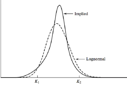
2.2.5 Implied Distribution

Brooks (2008) explains some of the distributional characteristics for financial time series and that is leptokurtosis and skewness. Leptokurtosis is the tendency for financial asset returns to exhibit fat tail distributions and a thinner but higher peak at the mean. It is often assumed that the residuals from a financial time series are normally distributed, but in practice the leptokurtic distribution is most likely to characterize a financial time

Theory

series and its residuals. Skewness indicates that the tails of a distribution are not of the same length. As mentioned in the preceding section the fact that the volatility smile exists implies that the underlying returns do not follow a lognormal distribution. The smile for equity options corresponds to the implied distribution that has the characteristics of leptokurtosis and skewness. Here is a comparison of the implied distribution for equities and the lognormal distribution.

Method

3 Method:

In this part of the thesis we are going to present different types of volatility forecasting models that will be used to conduct our research. We will also present ways to evaluate the different methods.

3.1 Forecasting Using Models

In order to calculate the future realized volatility on the OMXS30 we will estimate some models that can be used for volatility forecasting. The models that will be applied are those that can capture the different characteristics of volatility such as clustering, leverage effect, volatility persistence and other characteristics mentioned in chapter 2.2.

3.1.1 Forecasting Principle

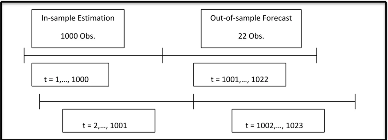
An important part of forecasting is to determine the amount of observations that the forecasts will be based on. We have chosen to follow the methodology of Becker et al. (2007) where 1000 observations are used to compute forecasts of the average 22-day ahead volatility. After the realized volatility has been computed the goal is to forecast the average volatility for the upcoming 22 days and to find out what forecasting model that performs the best. All model based forecasting will be conducted in the same way. Out of sample average forecasts for the upcoming 22 days will be performed using an in sample estimation period of 1000 days. We will apply a rolling window estimation methodology for our entire sample period so that the whole sample from 7th of May 2004 until the 5th of March 2014 will be covered. This means that the same number of observations will be used for our in-sample estimations, which is then used to create out-of-sample forecasts. All forecasts are then evaluated against the realized volatility that has been estimated using the log-range of the intraday high/low prices. Here is an overview of our in-sample estimations and our out-of-sample forecasts.

Method

Figure 3: Forecasting Methodology

The reason for generating out-of-sample forecasts over a 22-day period is to match the time-horizon with the SIX Volatility Index, our measure of implied volatility. The index value observed at time t represents a forecast of the average volatility of OMXS30 for the following 22 trading days (30 calendar days). The values displayed in the index are scaled to yearly volatility so it will be transformed to daily volatility to make the comparison with realized volatility easier.

3.1.2 Naïve Historical Model

This is one of the most straightforward and simple ways of forecasting volatility. The procedure is just to take the historically realized volatility and use it as a forward estimate of volatility. The reason for using this forecasting method is that the recently observed volatility is assumed to continue for the upcoming period (Canina & Figlewski 1993). Using the realized volatility to forecast uses the assumption that volatility is constant, evidence indicates that it is not (Figlewski 1997). We will not use this method solely as a forecasting tool as we will also use it as the benchmark model for the Theil-U statistic to evaluate the forecasting that is done with other more sophisticated forecasting methods.

The average daily realized volatility at time T can be calculated as 𝜎̂𝑇 = ∑ 𝑅𝑉_𝑡 𝑇 . (9) In-sample Estimation 1000 Obs. Out-of-sample Forecast 22 Obs. t = 1,…, 1000 t = 1001,…, 1022 t = 2,…, 1001 t = 1002,…, 1023

Method

Where 𝜎̂𝑇 denotes the forecast obtained from the naïve benchmark model that represents the average daily volatility from the previous T days, which in our case is 22. Information on how the realized volatility is calculated is available in section 2.1.2

.

3.1.3 Autoregressive Moving Average (ARMA)

The Autoregressive moving average model ARMA (p, q) is an important type of time series model that is normally used for forecasting purposes since it should be able to capture the persistent nature of volatility. In a research paper by Pong et al. (2004) they suggest that ARMA type models should capture the stylized features of volatility observed in financial markets. In short an Autoregressive Moving Average (ARMA) model is constructed by combining a Moving Average (MA) process together with an Autoregressive (AR) process. The Autoregressive Moving Average (ARMA) model lets the current value of a time series σ to depend on its own previous values plus a combination of current and previous values of a white noise error term. Hence, a desirable variable σ, which is volatility in our case, will demonstrate characteristics from a Moving Average (MA) process and an Autoregressive (AR) process if it is modeled after an ARMA model (Brooks 2008). The general ARMA (p, q) model is defined as: 𝜎𝑡 = 𝜇 + ∑ ∅𝑖 𝑝 𝑖=1 𝜎𝑡−1+ ∑ 𝜃𝑖 𝑞 𝑖=1 𝑢𝑡−1+ 𝑢𝑡 (10)

The MA (q) part of the ARMA (p, q) model is a linear combination of white noise error terms whose dependent variable σ only depends on current and past values of a white noise error term. A white noise process is defined in equation (11) and a MA (q) process for volatility is defined by equation (12).

𝐸(𝑢_𝑡) = 𝜇

𝑣𝑎𝑟(𝑢_𝑡) = 𝜎_𝑢2 ₍₁₁₎ 𝑢_𝑡−𝑟 = { 𝜎𝑢2 𝑖𝑓 𝑡 = 𝑟

Method

𝜎_𝑡= 𝜇 + ∑ 𝜃_𝑖 𝑞 𝑖=1

𝑢_𝑡−1+ 𝑢_𝑡 (12)

Equation (11) states that a white noise process has constant mean μ and variance σ2 _and zero autocovariance except at lag zero. In a MA (q) process the variable q is the number of lags of the white noise error terms. If we assume that the MA (q) process has a constant mean equal to zero, then the dependent variable σ will only depend on previous error terms (u).

The AR (p) part of the ARMA (p, q) model states that the current variable σ depends only on its own previous values plus an error term. The AR (p) process where p is the number of lags is defined by equation (13).

𝜎𝑡 = 𝜇 + ∑ ∅𝑖 𝑝

𝑖=1

𝜎𝑡−1+ 𝑢𝑡 (13)

An important and desirable property of an Autoregressive (AR) process is that it has to be stationary. An AR-process is stationary if the roots of the “characteristic equation” all lie outside the unit circle which in other words means that this process does not contain a unit root. The reason why stationarity is an important property is because if the variables of a time-series are non-stationary then they will exhibit the undesirable property that the impact of previous values of the error term (caused by a shock) will have a non-declining effect on the current value of σt as time progresses. This also

means that if the data is non-stationary the autocorrelation between the variables will never decline as the lag length increases. This property is in most cases unwanted and therefore it is important to take the stationary condition into consideration. There is a possibility that the statistical properties in our results obtained from our data will contain a unit root and therefore exhibit non-stationary behavior. Hence it is very important to test the stationarity condition in order to choose appropriate models. To test the stationarity condition we are going to perform the Augmented Dickey-Fuller

Method

unit root test (Brooks 2008). The ADF unit root test is an augmented version of the Dickey-Fuller test that was initially developed by Dickey & Fuller (1979).

As stated above an ARMA (p, q) model will demonstrate characteristics from a Moving Average (MA) process and an Autoregressive (AR) process and as a consequence of the stationarity condition of the AR model a non-stationary process cannot be modeled by an ARMA (p, q) model. Instead it has to be modeled by an Autoregressive Integrated Moving Average (ARIMA) model. The general ARIMA model is named the ARIMA

(p, d, q) model, where d is the number of times the variables are differentiated. An

ARIMA (p, 1, q) is defined as:

𝑦_𝑡+𝑠 = 𝑦_𝑡+ 𝛼₀𝑠 + ∑ 𝑒_𝑡+𝑖 𝑠 𝑖=1

(14)

𝑒_𝑡 = 𝜀_𝑡+ 𝛽₁𝜀_𝑡−1+ 𝛽₂𝜀_𝑡−2+ 𝛽₃𝜀_𝑡−3+ ⋯ (15)

The ARIMA model is modeling an integrated autoregressive process whose “characteristic equation” has a root on the unit circle and hence contains a unit root. It is therefore an appropriate model for volatility forecasting if a unit root is present.

3.1.4 Choice of ARMA Models

The first type of ARMA model we are going to use for forecasting realized volatility is the ARMA (2,1) model. This means that the current value of σt will depend on its

previous values σt-1 and σt-2 plus the previous error term ut-1 and the mean μ. The choice

of this model is motivated by the findings of Pong et al. (2004). They state that this particular model should capture the persistent nature of volatility when it is applied to high frequency data. More specifically, they conclude that two AR (1) processes can capture the persistent nature of volatility, which according to Granger & Newbold (1976) is equivalent to an ARMA (2,1) model. Pong et al. (2004) also mention a Autoregressive Fractional Integrated Moving Average (ARFIMA) model which also should be able to capture this feature and is therefore also a good model for forecasting realized volatility. The advantage of using this model is that if the persistence of volatility is very high then an ARFIMA model is more appropriate since it describes this long-lived feature better than an ARMA model. The authors however conclude that

Method

ARMA (2,1) and ARFIMA models perform equally well when the realized volatility is estimated using high frequency data. Since we are forecasting using a short forecasting horizon of 22 trading days then an ARMA (2,1) model with coefficients that indicates a short memory property would be more appropriate than an ARFIMA model. As later observed in section 5.2 our estimated ARMA (2,1) coefficients indicate a short-memory property and that the coefficients are stationary. Furthermore, since we use the log range estimator to estimate realized volatility to capture its intraday properties we find it motivated to choose an ARMA (2,1) model based on the research of Pong et al. (2004). The second type of ARMA model we are going to use is the ARIMA (1,1,1) model. By looking at the statistical properties of the estimated realized volatility insection 5.1 we observe that the realized volatility suffers from the presence of a unit root in some of the in-sample estimation periods. We therefore conclude that it would be appropriate to forecast future volatility with an ARIMA model to take care of the non-stationary property in our series. The ARIMA (1,1,1) model used in Christensen & Prabhala (1998) is chosen to complement the ARMA (2,1) model even though there are other types of ARIMA models. The motivation for the use of this specific model is to include both the MA and AR parts to better serve our purpose in forecasting volatility. More specifically we want these two parts to be included because of the persistent nature of volatility, hence it will follow some kind of MA and AR process.

3.1.5 Forecasting with ARMA (2,1)

To forecast the future volatility we denote

𝑓

𝑓𝑡,𝑠 = ∑ 𝑎𝑖𝑓𝑡,𝑠−𝑖+ ∑ 𝑏𝑗𝑢𝑡+𝑠−𝑗 𝑞 𝑗=1 𝑝 𝑖=1 (16) 𝑓_𝑡,𝑠 = 𝑦_𝑡+𝑠 𝑖𝑓 𝑠 ≤ 0 𝑢_𝑡+𝑠 = {_𝑢0 𝑖𝑓 𝑠 ≥ 0 𝑡+𝑠 𝑖𝑓 𝑠 < 0

Here the 𝑎_𝑖 and 𝑏_𝑗 coefficients capture the autoregressive part and the moving average part respectively. To understand how the forecasting procedure works by using an

Method

ARMA (p, q) model, which in our case is an ARMA (2,1) model we need to look at each part separately. The MA process part of the ARMA (p, q) model has a memory of

q periods and will die out after lag q. To see this one should understand that we are

forecasting the future value given the information available at time t and since the error term in the forecast period 𝑢_𝑡+𝑠, which is unknown at time t, is included in the forecast function it will then be equal zero. This means that the MA part of the forecasted ARMA (2,1) model will die out two steps into the future. In contrast to the MA part the AR process part of the forecast have infinite memory and will never die out and the forecasted value of interest will be based on previous forecasted values.

3.1.6 Forecasting with ARIMA (1,1,1)

The forecast function of the ARIMA (1,1,1) model will take the following form: 𝑓_𝑡,1 = 𝜎_𝑡+ 𝛼₁(𝜎_𝑡− 𝜎_𝑡−1)) + 𝛽₁(𝑢_𝑡− 𝑢_𝑡−1)

𝑓𝑡,2 = 𝑓𝑡,1+ 𝛼1(𝑓𝑡,1− 𝜎𝑡)) (17) 𝑓𝑡,𝑠 = 𝑓𝑡,𝑠−1+ 𝛼1(𝑓𝑡,𝑠−1− 𝑓𝑡,𝑠−2)

The 𝑓_𝑡,𝑠 symbol denotes the forecast made by the ARIMA (1,1,1) model at time t for s steps into the future. As in the ARMA (2,1) model the 𝑎𝑖 and 𝑏𝑗 coefficients denotes the autoregressive part and the moving average part respectively. Even though the intercept μ is included when estimating the model we have chosen not to include it in our forecast. The reason for this is that if the intercept is included it would lead to an everyday increasing value of the forecasted volatility, this also the case for the ARMA

(2,1) model.

3.2 Autoregressive Conditional Heteroskedastic (ARCH)

Models

3.2.1 ARCH Model

In chapter 2.2 we described some empirically observed features of volatility. One of these features was volatility clustering where large (small) absolute returns are followed by more large (small) absolute returns. In a study by Engle (1982) it is suggested that this particular feature could be modeled with an Autoregressive Conditional Heteroskedasticity (ARCH) model. Furthermore, since the volatility of an asset return

Method

series is mainly explained by the error term, the assumption that the variance of errors is homoscedastic (constant) is contradictory since these errors tend to vary with time. Therefore it makes sense to use the ARCH type models that does not assume that the variance of errors is constant. The ARCH model consists of two equations, the mean equation and the variance equation, which are used to model the first and the second moment of returns respectively (Brooks 2008).

The fact that the errors depend on each other over time states that volatility is autocorrelated to some extent. This supports the existence of heteroskedasticity and volatility clustering. Therefore under the ARCH model, the autocorrelation in volatility is modeled by allowing the conditional variance of the error term, (σ2), to depend on the

immediately previous value of the squared error. The ARCH (q) model, where q is lags of squared errors is defined as:

𝑦_𝑡= 𝛽₁+ 𝛽₂𝑥_2𝑡+ 𝛽₃𝑥_3𝑡+ 𝛽₄𝑥_4𝑡+ 𝑢_𝑡 𝑢_𝑡 ~ 𝑁(0, 𝜎_𝑡2_{) (18)}

Where equation (18) is the conditional mean equation and equation (19) is the conditional variance.

𝜎_𝑡2 _{= 𝛼}

0+ 𝛼1𝑢𝑡−12 + 𝛼2𝑢𝑡−22 + ⋯ + 𝛼𝑞𝑢𝑡−𝑞2 (19)

3.2.2 GARCH Model

The ARCH model however has a number of difficulties in the sense that it might require a very large number of lags q in order to capture all of the dependencies in the conditional variance. Hence it is very difficult to decide how many lags of the squared residual term to include. This also means that a lot of coefficients have to be estimated. Furthermore, a very large number of lags q can make the conditional variance explained by the ARCH model to take on negative values if a lot of the coefficients are negative, which is meaningless.

Method

A way to overcome these limitations and to reduce the number of estimated parameters is to use a generalized version of the ARCH model called the GARCH model. The GARCH model was developed by Bollerslev (1986) and Taylor (1986) independently and is widely employed in practice compared to the original ARCH model. The conditional variance in the GARCH model depends not only on the previous values of the squared error but also on its own previous values. A general GARCH (p, q), where p is the number of lags of the conditional variance and q is the number of lags of the squared error is defined by:

𝜎𝑡2 = 𝛼0+ ∑ 𝛼𝑖𝑢𝑡−𝑖2 𝑞 𝑖=1 + ∑ 𝛽𝑗𝜎𝑡−𝑗2 𝑝 𝑗=1 (20) 𝑦_𝑡= 𝛽₁+ 𝛽₂𝑥_2𝑡+ 𝛽₃𝑥_3𝑡+ 𝛽₄𝑥_4𝑡+ 𝑢_𝑡 𝑢_𝑡 ~ 𝑁(0, 𝜎_𝑡2_{) (21)}

The most common specification of the GARCH model according to Brooks (2008) is the GARCH (1, 1) model that is defined as:

𝜎_𝑡2 _{= 𝛼}

0+ 𝛼𝑢𝑡−12 + 𝛽𝜎𝑡−12 (22)

One of the shortcomings with the GARCH model is that even though it is less likely that it takes on negative values it is still possible for negative values of volatility to appear if no restrictions are imposed when estimating the coefficients. More importantly GARCH models can account for volatility clustering, leptokurtosis and the mean reverting characteristic of volatility. However they cannot account for asymmetries on returns (leverage effects) (Nelson 1991).

3.2.3 EGARCH Model

These restrictions were relaxed when Nelson (1991) proposed the Exponential GARCH (EGARCH) model. The advantage of this model is that the conditional variance will always be positive regardless if the coefficients are negative, but it will still manage to capture the asymmetric behavior. The conditional variance in an EGARCH model can be expressed in different ways but we have chosen to use the one specified in Nelson (1991), which is the same one that is programmed in Eviews, where the formula is given by:

Method ln(𝜎_𝑡2_{) = 𝜔 + 𝛽 ln(𝜎} 𝑡−12 ) + 𝛾 𝑒𝑡−1 √𝜎_𝑡−12 + 𝛼 |𝜀𝑡−1| √𝜎_𝑡−12 (23)

The EGARCH model has two important properties. First of all the conditional variance,

(σ2) will always be positive since it is logged and secondly the asymmetry is captured

by the (

𝛾

𝛾

negative relationship between volatility and returns. It also indicates that that negative shocks lead to higher volatility than positive shocks of equal size, which is exactly what leverage effect is and hence it gives support for its existence. The alpha coefficient (𝛼) captures the clustering effects of the volatility.

3.2.4 Choice of ARCH Models

Because of the limitations of the simple ARCH model described above we have decided in this thesis to concentrate on GARCH type models. The most common form of the GARCH model is the GARCH (1,1) model and this model is sufficient in capturing the volatility clustering in the data and could therefore be considered. However as mentioned above this model does not take the asymmetric behavior of volatility into account and since this feature is empirically observed in financial return data this particular model might not be the most appropriate one. We have already mentioned the use of the EGARCH model to capture this feature but other existing papers apply a variation of the standard GARCH (1,1) proposed by Glosten et al. (1993) known as the GJR model. The GJR model is designed to capture the asymmetric behavior to shocks, but it also shares some issues with the GARCH model. For example when estimating a GJR model the estimated parameters could in fact turn out to be negative which could lead to negative conditional variance forecasts and this is obviously not very meaningful. Therefore we have chosen to use the EGARCH model to avoid this and also because this model is the most likely to capture the most common characteristics of volatility discussed in chapter 2.2. To assure ourselves that asymmetric GARCH models are appropriate we will closely examine the gamma coefficient of the EGARCH.

3.2.5 EGARCH Model Estimation Using Maximum Likelihood

When estimating GARCH type models it is not appropriate to use the standard Ordinary

Least Square (OLS) since GARCH models are non-linear. We therefore employ the

Method

models. Based on a log likelihood function this method finds the most likely values of the parameters given the data. When using maximum likelihood to estimate the parameters you first have to specify the distribution of the errors to be used and to specify the conditional mean and variance. We will assume that the errors are normally distributed and given this the true parameters of our EGARCH model are obtained by maximizing its log likelihood function. A more thorough explanation of the maximum likelihood estimation is available in Verbeek (2004).

3.3 Quality Evaluation of Forecasts

In order to be able to conclude which forecasting method that performs the best in predicting future volatility some evaluation measures will be applied. These measures will determine the quality of the forecasted out-of-sample values against the observed values and will indicate what method that achieves the best results. Each forecasting methods predictive power and its informational content will also be evaluated.

3.3.1 Root Mean Square Error

The Root Mean Square Error (RMSE) has together with the Mean Square Error (MSE) been one of the most widely used as a measure of forecast evaluation. Their popularity is largely due to both measures theoretical relevance in statistical modeling (Hyndman & Koehler 2006). The RMSE is a so-called scale-dependent measure so it is useful when evaluating different methods that are applied to the same set of data, which fits the purpose of this thesis very well. RMSE is the same as the MSE measurement but with a square root applied to it. The measure is used to compare the predicted values against the actual observed values and the lower RMSE the better the forecast. The measure is expressed in the following way:

𝑅𝑀𝑆𝐸 = √ 1

𝑇 − (𝑇₁− 1)∑ (𝑦𝑡+𝑠− 𝑓𝑡,𝑠)2 𝑇

𝑡=𝑇1

(24)

Where T1 is the first forecasted out-of-sample observation and T represents the total

sample size including both in and out of sample. The variable ft,s is the forecast of a

Method

3.3.2 Mean Absolute Error

The evaluation measure called Mean Absolute Error (MAE) measures the average absolute forecast error. It distinguishes itself from the RMSE measure in being less sensitive to outliers (Hyndman & Koehler 2006). MAE measures the average of the absolute errors. As with RMSE there is no point at applying MAE across different series, but it is best used when evaluating different methods on the same data. Brooks & Burke (1998) state that MAE is an appropriate measure for forecast evaluation. The measure is given by the following formula:

𝑀𝐴𝐸 = 1

𝑇 − (𝑇₁− 1)∑|𝑦𝑡+𝑠− 𝑓𝑡,𝑠| 𝑇

𝑡=𝑇1

(25)

Again where T1 is the first forecasted out-of-sample observation and T represents the

total sample size including both in and out-of-sample. The variable ft,s is the forecast of

a variable at time t for s-steps ahead and yt is the actual observed value at time t.

3.3.3 Mean Absolute Percentage Error

An additional quality measure that we will use is the Mean Absolute Percentage Error (MAPE). An advantage with MAPE compared to the other measures that we have presented is that MAPE is expressed in percentage terms. The measure is recommended by Makridakis & Hibon (1995) as a superior evaluation measure for comparing results from different forecasting methods. The measure is expressed as following:

𝑀𝐴𝑃𝐸 = 100 𝑇 − (𝑇₁− 1)∑ | 𝑦_𝑡+𝑠− 𝑓_𝑡,𝑠 𝑦_𝑡+𝑠 | 𝑇 𝑡=𝑇1 (26)

Method

3.3.4 Theil Inequality Coefficient

Another popular evaluation measure is the Theil inequality coefficient known as the Theil-U statistic that was developed by Henri Theil (1966). The measure is defined as followed: 𝑈 = √∑ (𝑦𝑡+𝑠_𝑦− 𝑓𝑡,𝑠 𝑡+𝑠 ) 2 𝑇 𝑡=𝑇1 √∑ (𝑦𝑡+𝑠_𝑦− 𝑓𝑏𝑡,𝑠 𝑡+𝑠 ) 2 𝑇 𝑡=𝑇1 (27)

Where 𝑓𝑏_𝑡,𝑠 represents the forecast that is obtained from a benchmark model, usually a simple forecast performed using a Naïve model. The Theil-U statistic is performed in order to see if a benchmark model yields different results in comparison to more complex forecasting methods. A disadvantage of the Theil-U measure is that it can be harder to interpret compared to other measures such as MAPE (Madridakis et al. 1979). If the U-coefficient is less than 1 the model under consideration is more accurate than the benchmark model, if the U-coefficient is above 1 the benchmark model is more accurate and if the coefficient is equal to 1 both the considered model and the benchmark model are equally accurate.

3.3.5 Predictive Power

In order to investigate each models predictive power the following regression will be performed.

𝑅𝑉

̅̅̅̅_{𝑡+22= 𝛼 + 𝛽𝜎̂𝑡+ 𝜀𝑡 (28)}

Where 𝑅𝑉̅̅̅̅_𝑡+22 is the average realized volatility over 22 days, 𝜎̂_𝑡 is the 22-day average forecast performed at time t and 𝜀𝑡 is the error term of the regression.

The idea of performing this regression is to see how well the forecasted values can explain the observed future values of the realized volatility. How well the future values are explained is determined by the R2 _{measure. The forecasting method that produces}

the highest R2 has the best predictive power. The forecasts are considered to be unbiased if α is 0 and the estimate of β is close to 1 (Pagan & Schwert 1990) The problem with an

Method

data is homoscedastic and does not experience any correlation between the residuals over time. A problem with volatility is that it usually experiences heteroskedasticity and autocorrelation (Granger & Poon 2003). To account for these two features there is according to Newey & West (1987) the possibility to correct the standard errors.

3.3.6 Informational Content

Day & Lewis (1992) suggests that it can be useful to look at the informational content of each forecasting method in addition to their forecasting accuracy and predictive power. We will follow the procedure of Jorion (1995) when doing this. When investigating the informational content the purpose is to see whether the realized volatility of tomorrow can be explained at all by the forecasted values of today. To evaluate the informational content a modified version of equation (28) will be applied.

𝑅𝑉_𝑡+1= 𝛼 + 𝛽𝜎̂_𝑡+ 𝜀_𝑡 (29)

The difference from equation (28) is that 𝑅𝑉_𝑡+1 is the one-day ahead value of the realized volatility. 𝜎̂_𝑡 is the value that has been forecasted at time t and 𝜀_𝑡 is the error term. Since the procedure here is the similar to the test of predictive power we again have to account for assumed heteroskedasticity and autocorrelation by correcting the standard errors following the procedure of Newey & West (1979). The informational content is then evaluated by looking at the slope coefficient β and a β-value above 0 indicates a positive relationship.

Method

3.4 Additional Information in Implied Volatility

The last part of this thesis is to investigate if the implied volatility contains any additional information than what is captured by the time-series models. We will follow the procedure of Becker et al. (2007) by using the GMM (Generalized Method of

Moments) estimation method to determine if there is any additional incremental

information in SIXVX that cannot be captured by a combination of the model based forecasts. A decomposition of the SIXVX is necessary in this case and it can be expressed in the following way:

𝑆𝐼𝑋𝑉𝑋𝑡= 𝑆𝐼𝑋𝑉𝑋𝑡𝑀𝐵𝐹+ 𝑆𝐼𝑋𝑉𝑋𝑡∗ (30) The 𝑆𝐼𝑋𝑉𝑋_𝑡𝑀𝐵𝐹 _{part of the equation is the information that can be found in the different} model based forecasts. While 𝑆𝐼𝑋𝑉𝑋𝑡∗ is the part that might contain any information that can be useful for forecasting that is not captured by the model based forecasts.

If we store all the MBFs made at time t in a vector 𝜔𝑡, the relationship above can be transformed to a linear regression.

𝑆𝐼𝑋𝑉𝑋_𝑡= 𝛾₀+ 𝛾₁𝜔_𝑡+ 𝜀_𝑡 (31) 𝑆𝐼𝑋𝑉𝑋_𝑡∗ _{= 𝜀̂}

𝑡

In this form the (𝛾₀+ 𝛾₁𝜔_𝑡) part of the simple regression captures the information explained by the MBFs. If the SIXVX index would not contain any incremental information about the future realized volatility then the model based forecasts 𝑆𝐼𝑋𝑉𝑋_𝑡𝑀𝐵𝐹_{perform equally well as the SIXVX in forecasting future realized volatility.} This means that if any additional explanatory power exists in SIXVX then it is represented by the error term of the regression. More specifically the error term tells us if 𝑆𝐼𝑋𝑉𝑋_𝑡∗ _{can say anything about changes in future realized volatility which cannot be} anticipated by using MBFs

.

Furthermore, since 𝑆𝐼𝑋𝑉𝑋_𝑡∗ = (𝑆𝐼𝑋𝑉𝑋_𝑡− 𝑆𝐼𝑋𝑉𝑋_𝑡𝑀𝐵𝐹), then the simple regression above will ensure orthogonality between 𝑆𝐼𝑋𝑉𝑋_𝑡∗ _{and the vector containing the MBFs.} To use the GMM framework to estimate equation (31) we also need a set of instrument variables. A GMM estimation is performed in order to implement a set of pre-defined conditions. This is achieved by minimizing a function by varying the parameters that

Method

are to be estimated. A more formal explanation is that in order to estimate the parameters 𝛾 = (𝛾0, 𝛾1′) in equation (31) 𝑉 = 𝑴′𝑯𝑴 is minimized, where 𝑴 = 𝑇−1_(𝜀

𝑡(𝛾)′𝒁𝒕 is a K x 1 vector of moment conditions. H is a K x K weighting matrix and 𝒁_𝒕 represents a vector of instruments.

Becker et al. (2007) suggests that a vector of realized volatility should be included in the vector of instruments in addition to the regressors of equation (31). If the vector of instrument variables only contains the regressors the outcome of a GMM estimation will be the same as an OLS estimation.The realized volatility vector is defined as follows:

𝑅𝑉_𝑡+22= {𝑅𝑉̅̅̅̅_𝑡+1, 𝑅𝑉̅̅̅̅_𝑡+5, 𝑅𝑉̅̅̅̅_𝑡+10, 𝑅𝑉̅̅̅̅_𝑡+15, 𝑅𝑉̅̅̅̅_𝑡+22} (32) If the GMM is able to estimate the parameters of equation (31) that indicates that the residual of the equation is orthogonal to both the RV and 𝜔𝑡 vectors, it would imply that

𝑆𝐼𝑋𝑉𝑋_𝑡∗ does not contain any incremental information then what is captured by the MBFs. The orthogonality assumption is tested by looking at the J-statistic where the null hypothesis is that 𝑆𝐼𝑋𝑉𝑋_𝑡∗ _{is orthogonal to the instrument variables.}

Data

4 Data

In this chapter an overview of our dataset will be provided together with information about the SIX volatility index and the OMXS30 index.

4.1 General Data Description

We will use the SIX Volatility Index as a measure for implied volatility. For the application of the various time-series models we will use the OMXS30 index as our dataset. The volatility index is a fairly new index and data is only available since the 7th of May 2004. Therefore we will use data from that period until 5th _{of March 2014, this} will give us roughly 10 Years of data. Both the SIXVX and OMXS30 indices have been extracted from the Thomson Reuters Datastream database. The data has been managed in Excel and the models have been applied using Eviews.

4.2 OMXS30

The OMX Stockholm 30 Index is the leading equity index for Sweden. The index is a value-weighted index of the 30 most traded stocks on the Stockholm Stock Exchange. The index was introduced in September 1986 and its starting value was at 125. Dividends are not included and the index is revised two times every year.

4.3 SIXVX as a Measure of Implied Volatility

The SIX Volatility Index is based on OMXS30 index options with an average maturity of 30 calendar days. The index is calculated by rearranging the Black-Scholes option-pricing model so that the model is calculated backwards, thus the observed option prices will generate the volatility. The index is calculated every minute starting after the first

15 minutes on each trading day, the closing index per day is calculated at market close.

As a measure of risk free rate the STIBOR 90d rate is used and it remains fixed throughout the market day. The index value observed at time t could then be used as a forecast of the average volatility of OMXS30 for the following 30 calendar days (22 trading days) (SIX 2010). The index is provided by SIX financial information, a multinational financial data provider.

The methodology used when creating the index is the following:

1. The index is based on the implied volatility of OMX Stockholm 30 index options.