F
ORECASTING THE HOUSE PRICE INDEX
IN
S
TOCKHOLM COUNTY
2011-2014
A multiple regression analysis of four influential macroeconomic variables
School of Sustainable Development of Society and Technology
2011
Mattias Hedman, Peter Strömberg & Madeleine Broberg Tutor: Christos PapahristodoulouSpring Semester 199319941995 1996 1997 1998 1999 2000 2001 2002 2003 2004 2005 2006 2007 2008 2009 2010
A
BSTRACT
Course:
NAA301 Bachelor Thesis in Economics 15 ECTS
University:
Mälardalen University
School of Sustainable Development of Society and Technology, Västerås
Authors:
Mattias Hedman, Peter Strömberg & Madeleine Broberg
Tutor: Christos Papahristodoulou Pages: 28 Appendices: 6
Purpose of the research:
The purpose is to forecast the future trend of housing prices in Stockholm County 2011-2014 based on estimated slope coefficients of selected explanatory variables 1993-2010. Thereafter, the obtained forecast will be discussed with respect to other non-quantifiable concepts within behavioral economics.
Method:
Multiple regression technique with a deductive and explorative approach.
Empirical data:
Quantitative
Conclusion:
The future trend of housing prices in Stockholm County has been forecasted to be positively sloped throughout all the years 2011-2014, but in 2011, the forecast reveals that the increase of house prices will taper off. Nevertheless, behavioral economics reveals some insights about the trend on the housing market and that the house prices might include a portion of abnormal returns.
S
AMMANFATTNING
Kurs:
NAA301 Bachelor thesis in Economics 15 hp
Universitet:
Mälardalens Högskola
Akademin för hållbar samhälls- och teknikutveckling, Västerås
Författare:
Mattias Hedman, Peter Strömberg & Madeleine Broberg
Handledare: Christos Papahristodoulou Sidor: 28 Bilagor: 6 Syfte:
Syftet är att förutse den framtida utvecklingen av bostadspriserna i Stockholms län 2011-2014 baserade på beräknade lutningskoefficienter av valda förklaringsvariabler 1993-2010. Därefter kommer den erhållna prognosen att diskuteras i förhållande till andra icke-kvantifierbara begrepp inom beteendeekonomi.
Metod:
Multipel regressionsteknik med en deduktiv och explorativ strategi.
Empirisk data:
Kvantitativ
Slutsats:
Den framtida utvecklingen av bostadspriserna i Stockholms län har beräknats ha en positiv lutning inom samtliga år 2011-2014, men under 2011 visar också prognosen att ökningen av huspriserna kommer att avta successivt. Icke desto mindre avslöjar beteendeekonomi vissa insikter om utvecklingen på bostadsmarknaden och att huspriserna kan innehålla en andel abnorm avkastning.
A
CKNOWLEDGEMENTS
This paper would not have been possible without the help and co-operation of our tutor and associate professor, Christos Papahristodoulou. We are greatly indebted to him for all his guidance, patience and support, from the initial to the final stages of this paper. His precious time spent in helping us through this process is invaluable.
Lastly, we will also like to extend our deepest gratitude to our family members who have been a continuous support throughout the thesis.
Västerås 2011
T
ABLE OF CONTENTS
P
AGE 1 Introduction ... 1 1.1 Background ... 1 1.2 Problem area ... 1 1.3 Purpose ... 2 1.4 Target group ... 2 2 Methodology ... 3 2.1 Research approach ... 3 2.2 Choice of technique ... 3 2.3 Choice of theory ... 3 2.4 Data collection ... 3 2.4.1 Secondary sources ... 3 2.4.2 Primary sources ... 4 2.5 Validity of sources ... 4 2.6 Analysis method ... 43 Multiple regression technique ... 5
3.1 Multiple regression ... 5 3.2 Variables defined ... 5 3.3 General assumptions ... 6 3.4 Statistical assumptions ... 6 3.5 Data specification ... 6 3.6 Measurement ... 6 3.7 Equation ... 6 3.8 Theoretical slopes ... 7
3.9 Multicollinearity and Autocorrelation ... 8
4 Forecasting the independent variables ... 9
4.1 Real disposable income X2 ... 9
4.2 Real debt X1 ... 9
4.3 No. Houses/population X3 ... 9
4.4 Unemployment/population X4 ... 10
4.5 Behavioral economics ... 10
4.5.1 Various levels of rationality and herd behavior ... 10
4.5.2 Social status pressure ... 11
4.5.3 Positive confirmation bias ... 11
4.5.4 Lack of risk awareness ... 11
5 Multiple regression analysis ... 12
5.1 Testing the raw data of independent variables ... 12
5.1.1 Histograms and p-p plot ... 13
5.1.2 Simple regressions ... 14
5.2 Multiple regression analysis ... 15
5.2.1 Four variables ... 15
5.2.2 Three variables ... 16
5.2.3 Two variables ... 16
5.2.4 Autocorrelation ... 17
5.2.5 Correcting for (pure) autocorrelation ... 18
6 Forecasting ... 20
6.1 Forecasting independent variables ... 20
6.1.1 Debt X1 ... 20
6.1.2 Unemployment/population X4 ... 22
6.2 Repo rate and debt/disposable income probability intervals ... 23
6.3 Combing the results ... 23
6.4 Interpreting the result ... 26
7 Conclusion ... 28
Figure A3.1 – Correlation coefficient
Table 3.1 – Data connections to the independent variables and the dependent variable Table 3.2 – Data descriptions
Table 3.3 – Theoretical slope coefficients Table 5.1 – Skewness and Kurtosis Table 5.2 – Shapiro Wilk test ( = 0.05)
Table 5.3 – Regression statistics, dependent variable House Price index Y, four variables Table 5.4 – Regression statistics, dependent variable House Price index Y, three variables Table 5.5 – Regression statistics, dependent variable House Price index Y, two variables
Table 5.6 – Regression statistics, dependent variable House Price index Y, two variables (transformed)
Table 6.1 – An estimation of debt/disposable income in 2014 Table 6.2 – Unemployment & repo rate correlation
Table 6.3 – Regression statistics, dependent variable Unemployment/Population 1999-2010 Table 6.4 – Forecasted values 2011-2014
Table A1.1 – Raw Data 1993-2014
Table A1.2 – Mortgage rates from bank and institute 1993-2010 Table A1.3 – Mortgage duration weights
Table A2.1 – Collected data portrayed as indices Table A3.1 – Interest rate correlation
Graph 5.1 –Histogram of Debt X1 Graph 5.2 –P-P Plot of Debt X1
Graph 5.3 –Histogram of Disposable Income X2 Graph 5.4 –P-P Plot of Disposable Income X2 Graph 5.5 –Histogram of Houses/Population X3 Graph 5.6 –P-P Plot of Houses/Population X3
Graph 5.7 –Histogram of Unemployment/Population X4 Graph 5.8 –P-P Plot of Unemployment/Population X4 Graph 5.9 –Slope relationship Debt X1 to Y
Graph 5.10 – Slope relationship Disposable Income X2 to Y Graph 5.11 – Slope relationship Houses/Population X3 to Y
Graph 5.12 – Slope relationship Unemployment/Population X4 to Y Graph 5.13 – Histogram and normal distribution of residuals Graph 5.14 – P-P Plot of the standardized residuals
Graph 5.15 – Predicted standardized residuals Graph 5.16 – fit to actual Y, 1993-2010
Graph 6.1 – Geometric fit on income, incl. forecast, 1993-2014 Graph 6.2 – Disposable income (incl. forecast), 1993-2014 Graph 6.3 – Debt X1 (incl. forecast), 1993-2014
Graph 6.4 – Regression fit to actual X4, incl. forecast, 1993-2010 Graph 6.5 – X4 & repo rate, incl. forecast 1993-2014
Graph 6.6– Dependent variable (Y) and independent variables index 1993-2010, incl. forecasts and 25% probability intervals 2011-2014
Figures
Tables
Graph A3.1 – Housing prices Stockholm 1993-2010 Graph A3.2 – Population and supply Stockholm 1993-2010
Graph A3.3 – Disposable income Stockholm, 1993-2009, incl. 2010 forecast Graph A3.4 –Unemployment in Stockholm, 1993-2010
Graph A3.5 –Unemployment/population Stockholm, 1993-2010 Graph A3.6 – Debt/disposable income, 1993-2009
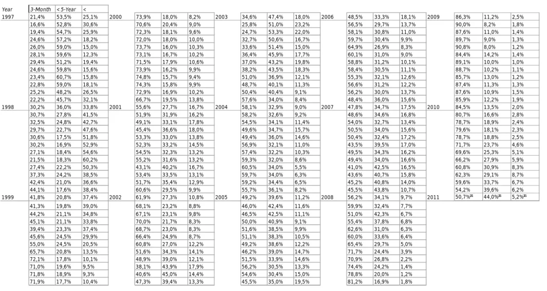
Graph A3.7 – Mortgage duration weights, 1997-2010 Graph A3.8 – 2-Year mortgage rates, 1993-2010 Graph A3.9 – 5-Year mortgage rates, 1993-2010 Graph A3.10 – 3-Month mortgage rates, 1993-2010
C
HAPTER OVERVIEW
I
NTRODUCTIONChapter one presents the background to the topic, problem area, purpose of the thesis and lastly the target group
1
M
ETHODOLOGYChapter two describes the research approach used, choice of technique and theory, data collection and the validity of the sources. Lastly the overall analysis method is depicted
2
M
ULTIPLE REGRESSION TECHNIQUEChapter three contains a short introduction to the multiple regression technique, a description of the variables and measurement, theoretical slopes and common complications. The Chapter ends with general and statistical assumptions
3
F
ORECASTING THE INDEPENDENT VARIABLESChapter four describes the process of forecasting the independent variables in order to estimate the future price index for houses. Lastly, a theoretical description of behavioral economics is presented
4
M
ULTIPLE REGRESSION ANALYSISChapter five contains testing of the raw data and the multiple regression analysis
5
F
ORECASTINGChapter six encompasses the forecasting of the independent variables. The result is presented and combined with the multiple regression equation and lastly discussed with respect to behavioral economics
6
C
ONCLUSIONConclusion with regards to the analysis carried out, fulfilling the purpose and answering the research questions of the thesis
1
I
NTRODUCTION
Chapter one presents the background to the topic, problem area, purpose of the thesis and lastly the target group The trend is your friend -An old saying
1.1
B
ACKGROUNDWhen information is complete and available, human decision making is assumed to be rational and correct according to the “neoclassical western economic literature” (Fromlet, 2001, p. 64). According to this perspective, the ideal human always achieve to maximize his or her utility (Ibid, p. 64). A market prevailed under a rational behavior assumption means that prices reflect their true values and that the market reacts fast to new information (Kindleberger & Aliber, 2005, p. 38). How we communicate, purchase goods and work has been highly dependent on the new integrated information technology. Through IT we can easily search for information about products and services, compare prices and make the necessary transactions more easily and less costly than before. Hessius (2000, p. 2) refers to this as “the naked economy”.
Rational thinking of steady price increases over time implies that the positive trend should continue in the market. According to Shiller, earlier high earned profits should continue to drive the prices and optimism up, even though this may result in overpricing of the good (Shiller R. J., 2002, p. 19).
1.2
P
ROBLEM AREAThe house prices have increased heavily in Sweden and even though the leverage has been quite high, small mortgage credit losses have been made during times of financial crises (2008-2009) (Central Bank, 2011, p. 7). In addition, a common trend in the mortgage market is that the duration of the interest rate is short and that the amortization level has decreased for most loans. An additional concern is that payment difficulties might occur if the unemployment would increase. This would lead to a lower demand for houses and further affect the prices negatively (Englund, 2011, p. 28). A heavy decline in the house prices has both in a historical and international perspective played a huge role in economic crises. A common reason for such crises has been due to increased indebtedness from expansionary fiscal/monetary policies and various international analysts have expressed concerns about the health of the market. The demand for houses is directly connected to variables such as income and unemployment, which then have an effect on the prices. The house prices are also affected by the quantity of new constructed houses and their respective building costs (Englund, 2011, p. 28).
The house prices can be very sensitive to changes in the repo rate (commonly also referred to as the interest rate set by the central bank) and there is a risk that the stability of the financial system will
be threatened if the house prices would fall substantially. Households would then experience difficulties to pay off their loans. If the prices would decline, the result might be similar to situations recently faced by other countries. Individual house values might then decline to levels less than the mortgage for the owners, which in turn could lead to personal insolvencies (Jönsson, Nordberg, & Fredholm, 2011, p. 136).
A recent survey amongst real estate agents showed that more agents believe in increasing prices in the Stockholm region compared to other areas in Sweden. In the conducted survey it was noted that the recently implemented mortgage ceiling had least effect in the Stockholm area (Nordberg & Soultanaeva, 2011, p. 356). Another survey conducted in April 2011 showed that 55% of the households believed that the house prices will increase next year; compared to 53% in March the same year. Even though the Central Bank has made a prognosis which shows by how much they plan to increase the repo rate, the households do not seem to believe in such increases (Lindqvist Sjöström, 2011).
A report was recently released by the Swedish Central Bank in order to clarify the situation on the real estate market in Sweden and whether there is a risk for a price bubble (Central Bank, 2011, pp. 7-9). Much due to the ongoing debate about the risks on the Swedish housing market, an interest in forecasting the future house prices in Stockholm County was found. Stockholm was selected due to the fact that it is the largest populated area in Sweden and that the mean prices for houses are the highest there (Ullman, 2007, p. 7).
1.3
P
URPOSEThe purpose is to forecast the future trend of housing prices in Stockholm County 2011-2014 based on estimated slope coefficients of selected explanatory variables 1993-2010 (A selection of appropriate explanatory variables can be found in Appendix 3). Thereafter, the obtained forecast will be discussed with respect to other non-quantifiable concepts within behavioral economics.
1.4
T
ARGET GROUPThis thesis should be relevant for; buyers and sellers of houses (consumers), real estate brokers, banks, macroeconomists and politicians.
2
M
ETHODOLOGY
Chapter two describes the research approach used, choice of technique and theory, data collection and the validity of the sources. Lastly the overall analysis method is depicted
2.1
R
ESEARCH APPROACHTo investigate this problem, a quantitative approach has been used. This approach is more appropriate for the purpose given that the analysis and data is based on numbers (Christensen, Andersson, Engdahl, & Haglund, 2001, p. 67).
A deductive and explorative approach has been used throughout the thesis. The deductive approach is used when existing theory can be applied to find and analyze the data (Saunders, Lewis, & A, 2009, p. 489), an explorative approach is used when considering specific values, trends, or distributions of variables. Once explored, the variables can be compared and analyzed in order to find relationships and interdependencies between them (Ibid, p. 429).
2.2
C
HOICE OF TECHNIQUEA multiple regression technique has been used to measure and quantify how a dependent variable Y is related to chosen independent variables (Anderson, Sweeney, & Williams, 2009, p. 534).
2.3
C
HOICE OF THEORYThe foundation of the paper is based on micro- and macroeconomic theory. The microeconomic theory of competitive markets and price mechanisms has been used to describe the market behavior and macroeconomic theory has been used to describe fiscal and monetary policies.
The topic of behavioral economics has also been included in the analysis due to the fact that individuals repeatedly overvalues assets and undervalues risk. The price of an asset should reflect the real value and risk in the long-run, nevertheless, in the short run, other psychological factors that seem to be immeasurable do have an effect on the prices. Behavioral finance illustrates that market efficiency does not transpire at all times (Lind H. , 2009, p. 84).
2.4
D
ATA COLLECTION2.4.1 SECONDARY SOURCES
Secondary data has been gathered from databases (ProQuest, Emerald and Google Scholar), Swedish Central Bank, Swedish Central Statistics Office (SCB), Student Association for Business and Society (SNS), Ekonomifakta.se and four Swedish Banks (Swedbank, SEB, Handelsbanken, Nordea). In addition, literature has been used from the University library.
2.4.2 PRIMARY SOURCES
No primary data has been used.
2.5
V
ALIDITY OF SOURCESAll quantitative data was gathered from SCB and the Swedish Central Bank. By Swedish law (2001:99), the responsibility of SCB is to provide official, objective and easily accessible statistics to the public (SCB-validity, 2011). Furthermore, the Swedish law (1986:223) states that the Swedish Central Bank must be objective in its operation and reporting (Riksbanken-validity, 2006). We realize that some of the variables collected from sources might include some human errors and that the attainment of a hundred percent accurate data is a “tedious” task.
2.6
A
NALYSIS METHODA selection of key macroeconomic variables.
An estimation of slope coefficients with the chosen technique.
Make use of variables that already are forecasted; remaining ones will be forecasted. Combine the results and estimate E(Y)
Discussion
All quantitative data has been processed, calculated, tabled and graphed in Microsoft Excel and SPSS. Note: some graphs contain dashed curves; these are to be interpreted as forecasted values.
3
M
ULTIPLE REGRESSION TECHNIQUE
Chapter three contains a short introduction to the multiple regression technique, a description of the variables and measurement, theoretical slopes and common complications. The Chapter ends with general and statistical assumptions
3.1
M
ULTIPLE REGRESSIONDespite the advantages of the multiple regression technique, it is important to point out that it reveals relationships, never causality (Hill & Lewicki, 2006, p. 346). In addition, when forecasting economic outcomes, the most difficult part is to be able to foretell where and when the turning points will be (Shiller R. J., 2008, p. 1). According to Hessius (2000, p. 3), if the focus has been on historical data to be able to predict what will happen in the future, the result will be very ambiguous after the turning points. During such times it is therefore better to focus on recent rather than historical data.
3.2
V
ARIABLES DEFINEDTable 3.1 illustrates the connections between the data, the independent variables and finally the house price index.
= (1 )( ) … (1 ) = × (1 ) × = × (1 ) × × ( / ) = / – Note: X3 is a ratio = / – Note: X4 is a ratio = × X1 - Debt Real
X2 - Disposable income Real
X3 - Number of houses/population
House Price Index (Y) Real
X4 - Unemployment/population Debt/disposable ratio Inflation Tax Nominal income No. Houses No. Unemployed Population Independent variables Collected data
Table 3.1 – Data connections to the independent variables and the dependent variable
3.3
G
ENERAL ASSUMPTIONS1) The demand equals the supply for all the years in a competitive market.
2) There are no substantial price deviations between various communities in Stockholm County.
3.4
S
TATISTICAL ASSUMPTIONS1) The regression model is linear in the parameters.
2) The values of the regressors, the X’s, are fixed in repeated sampling. 3) For given X’s, the mean value of the disturbance ui is zero.
4) If the X’s are stochastic, the disturbance term and the (stochastic) X’s are independent or at least uncorrelated.
5) The number of observations must be greater than the number of regressors. 6) There must be sufficient variability in the values taken by the regressors. 7) The regression model is correctly specified.
8) There is no exact linear relationship (i.e., multicollinearity) in the regressors.
9) The stochastic (disturbance) term ui is normally distributed.” (Gujarati, 2003, p. 335)
3.5
D
ATA SPECIFICATIONDebt/disposable ratio Percentage ratio describing the amount of debt over disposable income
Inflation General price increase of goods and services Tax Percentage income tax in Stockholm County Income Mean nominal income kr. in Stockholm County No. Houses Number of houses in Stockholm County No. Unemployed Number of employed in Stockholm County Population Number of inhabitants in Stockholm County
3.6
M
EASUREMENTThe data will be measured and analyzed in terms of indices, starting at 100% from the base year 1993. When using an index and linear relationship, the slope coefficients are denoted in units (Gujarati, 2003, p. 462).
3.7
E
QUATIONThe multiple regression technique fits a new regression line to the dependent variable Y based on the ordinary least squares (OLS) method. The equation given includes one intercept ( ) and one slope ( ) coefficient for each independent variable (Lind, Marchal, & Wathen, 2010, p. 506). The Table 3.2 – Data descriptions
multiple regression equation below represents the four selected variables that will be used for the multiple regression analysis.
= + + + +
The significance of the parameters will be tested with p-statistics, F-statistics, (Lind, Marchal, & Wathen, 2010, pp. 519, 521, 515), the slope coefficient and the overall explanatory power with the adjusted coefficient of determination (R2adj) (Gujarati, 2003, p. 217).
3.8
T
HEORETICAL SLOPESThe leveraging phenomena and the economic situation of households have been discussed extensively by the Central Bank (2011) & SNS (2011). Debt financing increases the purchasing power; hence it affects the overall house prices (Central Bank, 2011, p. 8). Theoretically, the level of debt is positively correlated with the house prices.
According to several investigations about the housing market, average income is repeatedly referred to as an important variable (Central Bank, 2011, pp. 17, 71, 244); macroeconomic theory further supports this statement that when the disposable income increases, overall prices also increase (Case & Fair, 2007, p. 56). Theoretically, the level of disposable income is positively correlated with the house prices.
The law of demand and supply states that increased demand leads to a higher market price in the short term. An increased market price should also lead to increased supply, which in the long-run should stabilize the market into equilibrium (Pindyck & Rubinfeld, 2009, p. 48). When there is an excess demand (or scarcity), prices should increase (Pindyck & Rubinfeld, 2009, p. 596). Since the number of houses per person in Stockholm has decreased (appendix 3), it can be expected that this difference has affected the prices for houses. Theoretically, the amount of houses/population is negatively correlated with the house prices.
Continuing the path of demand; unemployment is another factor relevant when considering the demand for houses. When the unemployment is high, fewer buyers exist on the market, thus leading to decreased demand for houses (Englund, 2011, p. 28). Theoretically, the level of unemployment is negatively correlated with the house prices.
House prices (Y)
X1 – Debt +
X2 - Disposable income +
X3 - Number of houses/population
X4 - Unemployment/population
3.9
M
ULTICOLLINEARITY ANDA
UTOCORRELATIONCommon when conducting a multiple regression analysis is that some or at least few of the independent variables are correlated with each other. “When two variables are correlated, it means that they both convey essentially the same information” (Motulsky, 2002). In such a case, both variables might not individually contribute to the model, but together their contribution might be large. If both of the variables would be removed, the fit would probably be less (Motulsky, 2002), an issue commonly referred to as multicollinearity. In addition, one problem with multicollinearity is that an individual high p-value can be very misleading. The individual variable might very well be important to the result. Multicollinearity is measured by the variance inflation factor (VIF) (Ibid, p. 527).
Autocorrelation is another important issue to consider. If it is positive or negative, autocorrelation means that the regression outcome is affected by the past (Lind, Marchal, & Wathen, 2010, p. 622). Autocorrelation is measured using the Durbin-Watson Statistic (Ibid, p. 622). Both tests will be applied in the analysis and adjusted if existent.
4
F
ORECASTING THE INDEPENDENT VARIABLES
Chapter four describes the process of forecasting the independent variables in order to estimate the future price index for houses. Lastly, a theoretical description of behavioral economics is presented
4.1
R
EAL DISPOSABLE INCOME X2Three variables are needed in order to forecast the real disposable income (income, tax, inflation). In terms of tax it will be assumed that it is equal to the mean 1993-2010 and constant throughout 2011-2014. In addition, it has been assumed that all individuals in Stockholm County pay the same amount of tax. An inflation prognosis has been obtained from the Central Bank for 2011-2014 (Central_Bank_forecast, 2011). In order to forecast the real disposable income, the geometric mean approach has been used. “The geometric mean answers the question; what was your average compound return per year over a particular period?” (Ross, Westerfield, & Bradford, 2008, p. 320), thus it is assumed that the disposable income has grown exponentially from 1993-2009. Using the above mentioned three variables, we will estimate the real disposable income between the years 2011-2014 under the assumption that the income will continue to grow according to the compounded level 1993-2009.
4.2
R
EAL DEBTX
1Jansson and Persson (2011, p. 13) state that there is a relationship between growing house price bubbles and increasing leverage. The interest rate is commonly portrayed as the cost of holding money and when the repo rate decreases, money demanded is likely to increase due to relatively lower cost of borrowing. Therefore, in essential macroeconomic theory, it is said that the quantity of money demanded is inversely related to the interest rate (Case & Fair, 2007, p. 229).
Debt is calculated from four variables, nominal income, tax, inflation and debt/disposable income (ratio) for Sweden, which is assumed being the same for Stockholm County. From the preceding estimation of the real disposable income, the debt/disposable income ratio has been used to rearrange and calculate the debt in real terms between the years 1993-2009. By using the already made prognosis of the debt/disposable income (ratio) 2010-2013 (Central bank_forecast_2, 2010), a debt estimate will be forecasted for 2010-2013.
4.3
N
O.
H
OUSES/
POPULATIONX
3The No. houses/population is comprised from two variables, the population and the number of houses. A population prognosis was obtained from the regional planning office in Stockholm for 2011-2014 (2010). The No. of houses will be estimated with an ordinary time regression. It is moreover assumed that the houses in Stockholm County are of “similar characteristics” and that
the quantity of houses will continue to grow with the same average rate as between the years 1993-2009.
4.4
U
NEMPLOYMENT/
POPULATION X4We are aware that demographics play a significant role when determining the unemployment rate and that our variable used for the forecast might not portray a true picture. The assumption behind using this variable as such is that the weights of various ages in the demographic data have remained constant. It should also be noted that the unemployment in Stockholm County has been on average 1.05% lower than in the rest of Sweden during the past five years and that the correlation between these years is 95% (Ekonomifakta-unemployment, 2011).
An important question in macroeconomics is what influences the interest rate decision. Two of the main goals of the Central Bank are high levels of output and employment and a low rate of inflation. “The Central Bank is likely to lower the repo rate (and thus increase the money supply) during times of low output (high unemployment) and low inflation” (Case & Fair, 2007, p. 304). Due to the high correlation between unemployment 1999-2010 and the repo rate, this variable will be forecasted from the prognosticated repo rate. It is assumed that this relationship continues throughout 2011-2014 and that the labor force will continue to grow proportionally with the population.
4.5
B
EHAVIORAL ECONOMICS4.5.1 VARIOUS LEVELS OF RATIONALITY AND HERD BEHAVIOR
When households observe that others are profiting from sales of houses, a “follow-the leader process” comes into place. A market situation like this may lead to increased credit amounts allowed by the banks, since they do not want to lose market share to competitors. When the trend is upward sloping, earning money never seems to be easier. During such times everybody wants to enjoy the high capital returns, leading the market towards violating some of the rational behavior (Kindleberger & Aliber, 2005, p. 29).
When an individual is basing his or hers beliefs about the future of what happened in the past, it is called adaptive expectations. Distinguishing adaptive expectations from rational expectations, the rational expectations mean that the future price mirrors the current prices (Kindleberger & Aliber, 2005, p. 38).
Some distinctions can be made between the individual level and the group level. One of them is when practically everybody in the market changes their mind at the same time and move simultaneously as a “herd”. The phenomenon is referred to as the mob psychology assumption. On the other hand, people can amend their beliefs about the environment in different periods as part of an ongoing procedure. The change in mind will be logical at first but when more and more people are added, it results in irrational behavior. This process as it seems, goes faster and faster once started
(Kindleberger & Aliber, 2005, pp. 41-42). Purchasing a house that is in a higher price level than what the individual income allows is another irrational behavior. This can be flourished by impatience which might have a connection with “herd behavior” (Lind H. , 2009, p. 87). In addition, the individual might feel that if he or she does not purchase a house now, the belief might be that owning a house in the future is impossible due to increased prices. (Case & Shiller, 2003, p. 325).
4.5.2 SOCIAL STATUS PRESSURE
To be recognized as “successful”, individuals must be able to afford today’s standards of living and social goal. The standard is measured as the level of material goods; the higher quality goods possessed, the better the individual’s status. When individuals compare themselves with others who might have reached a higher level of quality goods and social status, the result is likely to lead to decreased self-esteem. In order to avoid this lowering in self-esteem, an individual has a drive to “keep up with the Joneses” consumption level. This is referred to as the demonstration effect (McCormick, 1983, p. 1126).
4.5.3 POSITIVE CONFIRMATION BIAS
When humans want something to be in a certain way, they usually look for the factors that support their beliefs and disregard other information that states otherwise; this psychologists call positive confirmation bias (Jones & Sugden, 2001, p. 59).
4.5.4 LACK OF RISK AWARENESS
According to a survey conducted by Case and Shiller (2003, p. 345), people that own houses seem to think that the stock exchange is more risky than the housing market, despite that the housing market might be equally risky when people purchase houses grounded on the belief that the prices will continue to increase the next day. This behavior is often the start of a chain reaction leading to abnormal prices. In addition, if households are decreasing their amortizing when the interest rate is low, it is a sign of higher risk taking (Lind H. , 2009, p. 87).
Usually individuals believe that their city is more attractive than others. What they do not consider is that there is a risk that other cities will become more popular. This is referred to as the uniqueness bias (Shiller R. J., 2008, p. 5).
Consumers have a tendency to be confident about their purchasing decision, even though they lack the control over the situation. Some people think that they can control their own situation, but in real life it is an illusion of overconfidence which increases the risk-taking (Fromlet, 2001, p. 66). Rationality is thus not a description of how the world works; it is an assumption of how the world should work (Kindleberger & Aliber, 2005, p. 40).
5
M
ULTIPLE REGRESSION ANALYSIS
Chapter five contains testing of the raw data and the multiple regression analysis
5.1
T
ESTING THE RAW DATA OF INDEPENDENT VARIABLESThe skewness test of the data yielded that all independent variables were not symmetrically distributed around the mean (0), but all of them fell inside the critical values of ± 1.030 (two-tailed,
= 0.05). Debt was positively skewed and remaining independent variables were negatively skewed.
The kurtosis critical values are -1.27 and +2.56 ( = 0.05) which indicated that X2 fell outside the lower critical value. It was noted that X1, X2, X4 were platykurtic and X3 leptokurtic. According to statistics, kurtosis risk means that the spread of the data is wider than in a normal distribution (Jobson, 1999, p. 52). Due to this fact, a Shapiro Wilk test was carried out, which performs better for n < 50 (Cullinan, et al., 2001, p. 72). This test clarifies further whether the data is from a normal distribution or not. H0 was stated: p-value > and H1: p-value < .
X1 - Debt 0.929 18 0.183
X2 - Disposable income 0.883 18 0.030
X3 - No. houses/population 0.939 18 0.276
X4 - Unemployment/population 0.955 18 0.513
It was noted that the p-value > , hence H0 could not be rejected (data is normally distributed) for
all variables except X2. X1 - Debt
X2 - Disposable income X3 - No. houses/population X4 - Unemployment/population
Skewness Kurtosis
Table 5.1 – Skewness and Kurtosis
Statistic df p-Value
Independent variables
Table 5.2 – Shapiro Wilk test ( = 0.05) 0.258 -0.505 -0.539 -0.355 -1.262 -1.330 0.792 -0.928 Independent variables
5.1.1 HISTOGRAMS AND P-P PLOT
Graph 5.1 –Histogram of Debt X1 Graph 5.2 – P-P Plot of Debt X1
Graph 5.3 –Histogram of Disposable Income X2 Graph 5.4 – P-P Plot of Disposable Income X2
Graph 5.5 –Histogram of Houses/Population X3 Graph 5.6 – P-P Plot of Houses/Population X3
The cumulative p-p plot is portraying the empirical cumulative density function (CDF) plotted against the theoretical normal CDF values. In these p-p plots µ = sample mean, = sample standard deviation. If plotted values are roughly linearly they follow a theoretical normal distribution (Cullen & Frey, 1999, p. 141). As was noted, the observed cumulative probability of disposable income deviates around 0.45.
5.1.2 SIMPLE REGRESSIONS
The following regressions were made with the dependent variable house price index (Y) and each respective independent variable. The empirical findings support the economic theoretical slope relationship against house prices discussed in 3.6.
With regard to recently presented skewness, kurtosis, Shapiro Wilk test and p-p plots, all four variables were included in the multiple regression analysis.
Y = 1,164 x - 0,074 R² = 0,983 100% 150% 200% 250% 300% 350% 50% 100% 150% 200% 250% 300% H o u se P ri ce s Y Debt X Y = 1,164 x - 0,074 R² = 0,983 100% 150% 200% 250% 300% 350% 50% 70% 90% 110% 130% 150% H o u se P ri ce s Y Disposable income X Y = -35,151 x + 36,059 R² = 0,663 100% 150% 200% 250% 300% 350% 93% 94% 95% 96% 97% 98% 99% 100% 101% H o u se P ri ce s Y Number of houses/population X Y = -1,271 x + 2,806 R² = 0,121 100% 150% 200% 250% 300% 350% 20% 30% 40% 50% 60% 70% 80% 90% 100% 110% H o u se P ri ce s Y Unemployment/population X
Graph 5.9 – Slope relationship Debt X1 to Y Graph 5.10 – Slope relationship Disposable Income X2 to Y
5.2
M
ULTIPLE REGRESSION ANALYSIS5.2.1 FOUR VARIABLES
When the first multiple regression was conducted with four independent variables, the slopes of the regression did not depict their expected signs. For example, note that X3 had a positive slope when it in fact should have had a negative one, as that estimate incorrectly illustrates. The same applies for X2, which was negatively related to Y but should have been positive; that is, when the income increases, the house prices should also increase. The reason for incorrect slopes could be explained by the high multicollinearity of the test (for in depth calculations see Appendix 4). The critical limit usually is drawn at 10 for the VIF (Field, 2000, p. 153).
Based on the findings, the individual p-values and F-value were not reliable. The high VIF-values indicated that the variables were correlated with one or some of the other variables. This in turn distorts the statistical significance as the variables convey the same information. It was noted that X2 had the highest VIF of 89.35. Another consideration can be referred to what was mentioned earlier, that this variable had the worst fit on the p-p line. Remember also that we could not state that X2 was normally distributed in the Shapiro Wilk test. As a result, a second regression was made excluding it. Multiple R 0,997 R Square 0,994 Adjusted R Square 0,993 Standard Error 0,059 Observations 18 ANOVA table SS df MS F Significance F DW Regression 7,8617 4 1,9654 568 1,92E-14 2,34 Residual 0,0450 13 0,0035 Total 7,9067 17
variables coefficients std. error t (df=13) p-value 5% lower 5% upper VIF
Intercept -3,6574 2,0708 -1,766 1,01E-01 -3,7898 -3,5251
Debt X 1,3723 0,1977 6,942 1,02E-05 1,3597 1,3849 64,765
Unemployment/population X -0,5498 0,2601 -2,114 5,44E-02 -0,5664 -0,5332 11,399
Number of houses/population X 4,5226 1,7311 2,613 2,15E-02 4,4119 4,6333 3,623
Disposable income X -0,6160 0,8798 -0,700 ,4961 -0,6723 -0,5598 89,350
42,284 Mean VIF
5.2.2 THREE VARIABLES
Upon the next regression it was found that X3 still had the incorrect slope (positive). The other two slopes had the relationships that were predicted earlier according to theory. When X2 was excluded, the VIF-values decreased substantially and the individual p-values became more statistically significant. The F-value also increased compared to the previous regression, which is positive, but X1 and X3 still showed signs of multicollinearity. X3 was least significant; furthermore it had the highest VIF and was the only variable with the incorrect slope sign, hence another regression test was made excluding it.
5.2.3 TWO VARIABLES
The slopes of both variables in this regression had the correct signs, i.e. if debt increases with 1 unit, the house price index increases with 1.1342 units, or if unemployment increases with 1 unit, the house price index will decrease with 0.3439 units. The VIF-values indicated very low multicollinearity and the individual p-values and the overall F-significance were very low.
Multiple R 0,997 R Square 0,994 Adjusted R Square 0,993 Standard Error 0,058 Observations 18 ANOVA table SS df MS F Significance F DW Regression 7,8600 3 2,6200 785 7,88E-16 2,25 Residual 0,0467 14 0,0033 Total 7,9067 17
variables coefficients std. error t (df=14) p-value 5% lower 5% upper VIF
Intercept -4,4541 1,6984 -2,622 2,01E-02 -4,5626 -4,3457 Debt X 1,2377 0,0451 27,440 1,43E-13 1,2348 1,2405 3,499 Unemployment/population X -0,3767 0,0794 -4,744 3,14E-04 -0,3818 -0,3716 1,103 Number of houses/population X 4,6586 1,6886 2,759 ,0154 4,5508 4,7664 3,577 2,726 Mean VIF Multiple R 0,995 R Square 0,991 Adjusted R Square 0,990 Standard Error 0,069 Observations 18 ANOVA table SS df MS F Significance F DW Regression 7,8346 2 3,9173 815 5,01E-16 1,35 Residual 0,0721 15 0,0048 Total 7,9067 17
variables coefficients std. error t (df=15) p-value 5% lower 5% upper VIF
Intercept 0,2263 0,0970 2,332 ,0340 0,2201 0,2324
Debt X 1,1342 0,0300 37,744 2,77E-16 1,1322 1,1361 1,078
Unemployment/population X -0,3439 0,0942 -3,649 ,0024 -0,3499 -0,3379 1,078
1,078 Mean VIF
Table 5.4 – Regression statistics, dependent variable House Price index Y, three variables
Another positive sign was that the F-value had increased from the two previous regressions and that it still was higher than the critical value of 3.68 ( = 0.05). The t-values for all variables fell outside their critical limits of ± 2.131 (2-tailed, = 0.05), therefore they were statistically significant. Conceptually, the variables had individual explanatory power on the house price index. The regression equation is: = 0.2263 + 1.1342 0.3439 .
With correct slopes, low VIF-values, significant t-values, small p-values and a high F-value, it now made sense to look at the Durbin Watson (for in depth calculations see Appendix 5). The obtained Durbin Watson was 1.35, which lies in between the lower 1.05 and upper 1.53 critical values. This means that the result was inconclusive and that further tests must be conducted to assess whether autocorrelation exists in the data or not.
5.2.4 AUTOCORRELATION
Plotting the standardized residuals against predicted standardized residuals yielded graph 5.15 in which the residuals appeared as random. The histogram (graph 5.13) “resembles” a normal distribution but depicted below is also a p-p plot (graph 5.14) of the residuals which slightly deviates around 0.35 and 0.55.
Graph 5.13 – Histogram and normal distribution of residuals Graph 5.14 – P-P Plot of the standardized residuals
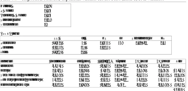
In order to test whether the data had pure autocorrelation or not, H0 was stated: = 0; that is, no
present negative or positive autocorrelation and H1: different from 0, that statistically significant
positive or negative autocorrelation is present (Gujarati, 2003, p. 470).
was estimated (Gujarati, 2003, p. 469), which resulted in 0.289098354. can also be estimated with respect to the Durbin Watson test (Gujarati, 2003, p. 481), which yielded 0.325. A more accurate measure stated by Gujarati is that “ is the slope coefficient in the regression of ut on ut-1”
(Gujarati, 2003, p. 450). This resulted in = 0.3111631 (for in depth calculations see Appendix 6).
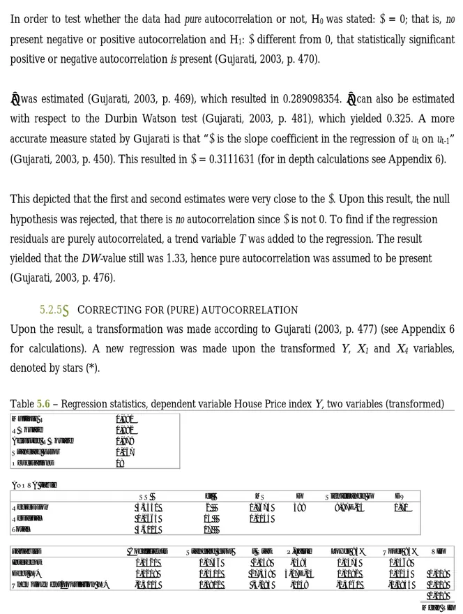
This depicted that the first and second estimates were very close to the . Upon this result, the null hypothesis was rejected, that there is no autocorrelation since is not 0. To find if the regression residuals are purely autocorrelated, a trend variable T was added to the regression. The result yielded that the DW-value still was 1.33, hence pure autocorrelation was assumed to be present (Gujarati, 2003, p. 476).
5.2.5 CORRECTING FOR (PURE) AUTOCORRELATION
Upon the result, a transformation was made according to Gujarati (2003, p. 477) (see Appendix 6 for calculations). A new regression was made upon the transformed Y, X1 and X4 variables, denoted by stars (*).
After the correction, the Durbin Watson statistic increased to 1.71, which was larger than the upper critical value of 1.53. It was acknowledged that the autocorrelation had been removed. The slopes were still theoretically correct, even though the individual “strengths” of the slopes had been slightly altered. If X1* increases with one unit holding X4* constant, Y* increases by 1.1208 units. If X4* increases with one unit holding X1* constant, Y* would decrease with 0.3003 units. The VIF-values had decreased further down to 1.019, therefore we could assume also no multicollinearity.
Multiple R 0,991 R Square 0,982 Adjusted R Square 0,979 Standard Error 0,067 Observations 18 ANOVA table SS df MS F Significance F DW Regression 3,5350 2 1,7675 399 9,87E-14 1,71 Residual 0,0664 15 0,0044 Total 3,6014 17
variables Coefficients Standard error t Stat P-value Lower 95% Upper 95% VIF
Intercept 0,1521 0,0746 2,039 ,0594 0,1474 0,1569
Debt X * 1,1208 0,0410 27,338 3,27E-14 1,1182 1,1234 1,019
Unemployment/population X * -0,3003 0,0912 -3,293 ,0049 -0,3061 -0,2945 1,019
1,019 Mean VIF Table 5.6 – Regression statistics, dependent variable House Price index Y, two variables (transformed)
Graph 5.16 – fit to actual Y, 1993-2010
The individual p-values were still very low and the significance of the t-values for all variables except the intercept fell outside the critical limits of ± 2.131 (2-tailed, = 0.05). If we would have chosen a significance of 10% (2-tailed, = 0.10), the critical value would have been at 1.753. Since the t-value of the intercept was only slightly below the critical 5% value, consequently we did not see a problem in this model.
When we were observed the Analysis of Variance (ANOVA), we noted that the F-statistic was 399 and still larger than the critical value of 3.68 ( = 0.05). If it is higher than the critical value it is usually assigned that the regression model will be of use to assess the dependent variable (Lind, Marchal, & Wathen, 2010, p. 518).
The computed R2 was 0.982. Adjusted for its degrees of freedom (R2adj) it still remained very high
(0.979). The coefficient of multiple determination measures the fit of a linear regression. If the value is one, the regression line falls exactly on the dependent variable, that is, without any errors. If the value is zero, there is no association between the dependent and independent variables (Lind, Marchal, & Wathen, 2010, p. 515).
Consequently, this produced the following transformed equation; = 0.1521 + 1.1208 0.3003
Plotted in graph 5.16 is the fit of the regression (dashed in blue) to the actual values (red). The relatively good fit has led us to believe in the strength of the model and that it can be used to forecast the future house price index in Stockholm County 2011-2014. 90,0% 110,0% 130,0% 150,0% 170,0% 190,0% 210,0% 230,0% 250,0% 270,0% 290,0% 1993 1994 1995 1996 1997 1998 1999 2000 2001 2002 2003 2004 2005 2006 2007 2008 2009 2010
6
F
ORECASTING
Chapter six encompasses the forecasting of the independent variables. The result is presented and combined with the multiple regression equation and lastly discussed with respect to behavioral economics
6.1
F
ORECASTING INDEPENDENT VARIABLES6.1.1 DEBT X1
When data was obtained for years 1993-2009, the variables inflation and tax for year 2010 were already available. By observing that the growth of income had been fairly stable for the last 18 years (graph 6.1 green), the preceding income was calculated with the geometric mean method. It was found that the geometric growth of income 1993-2009 was 3.40% annually (nominal terms). Assuming the same compounded growth of income, the missing 2010-2014 year data was forecasted (graph 6.1, dashed in green). The dashed blue line shows the geometric fit to income 1993-2009.
After tax and inflation adjustments, it was noted that the disposable income had increased with 41.2% 1993-2009 (graph 6.2). It is forecasted to grow with 50% in 2014 compared to 1993. The debt/disposable income ratio (graph 6.3 in purple) has been obtained from the Central Bank for the years 1993-2013. By using the disposable income debt (dark green) could be expressed in numerical terms. As mentioned before, the debt variable is based on income, tax, inflation and the debt/disposable income (ratio) and only the disposable income was missing for 2010. In graph 6.3, the debt level in 2010 is dashed, meaning that the value has been forecasted despite already obtained values for tax, inflation and debt/disposable income (ratio).
Graph 6.1 – Geometric fit on income, incl. forecast, 1993-2014
Nominal terms
Graph 6.2 – Disposable income (incl. forecast), 1993-2014
Real terms 100% 120% 140% 160% 180% 200% 220% 240% 1993 1994 1995 1996 1997 1998 1999 2000 2001 2002 2003 2004 2005 2006 2007 2008 2009 2010 2011 2012 2013 2014
Graph 6.3 – Debt X1 (incl. forecast),1993-2014
Real terms 100,0% 105,0% 110,0% 115,0% 120,0% 125,0% 130,0% 135,0% 140,0% 145,0% 150,0% 1993 1994 1995 1996 1997 1998 1999 2000 2001 2002 2003 2004 2005 2006 2007 2008 2009 2010 2011 2012 2013 2014 0,0% 50,0% 100,0% 150,0% 200,0% 250,0% 300,0% 350,0% 1993 1994 1995 1996 1997 1998 1999 2000 2001 2002 2003 2004 2005 2006 2007 2008 2009 2010 2011 2012 2013 2014
It should be noted that the very last value (turquoise) has been estimated without any calculation. The logic behind this estimation is that the repo rate (orange) is forecasted to increase through the next coming years, meaning that the debt/disposable income (ratio) should decline in the long run. Economic theory inversely relates the relationship between the repo rate and debt. Nevertheless, when looking at the forecast for the repo rate and the debt/disposable income it makes no rational sense. The repo rate is expected to increase and the debt/disposable income as well, even though it would be rational to assume a negative relationship. The reason for this could perhaps be explained by some behavioral factors. When viewing graph 6.3, one can note that the debt has been increasing at a rapid pace during the years. The households engage in risk behavior when increasing their debt due to the fact that they believe that the house prices will continue to increase. Perhaps individuals are being impatient and thinking that they can miss their chances of affording a house if they do not seize the chance when the interest rate is historically low as described by Case and Shiller (2003, p. 325).
Even though the Central Bank has made a prognosis of the Repo rate, the households do not seem to believe that the repo rate will increase in the same pace as the Central Bank has indicated (Lindqvist Sjöström, 2011). As a result, individuals keep on borrowing. The phenomenon could further be connected and perhaps explained by some level of positive confirmation bias (Jones & Sugden, 2001, p. 59) and overconfidence (Fromlet, 2001, p. 66) resulted from such behavior.
The demonstration effect is also a possible explanation for the prognosis, as people are constantly comparing and thinking about what others have bought and are planning to buy. For example, all “Svenssons” wants to keep up with the other “Svenssons” level of wealth and status, this kind of thinking may also have caused the leverage to raise and therefore also indirectly the house prices (McCormick, 1983, p. 1126).
According to adaptive expectations, individuals can observe that the prices of houses have increased, which then would impose that higher leveraging involves less risk (Kindleberger & Aliber, 2005, p. 38). But with the fact in mind that the interest rate is expected to increase, the risk of generating a negative debt spiral also increases. In addition, what the households do not think about is what will happen if the prices of houses will fall and the repo rate will increase. Also the real estate agents seem to believe in increasing house prices in Stockholm County (Nordberg & Soultanaeva, 2011, p. 356) even though the price increase has been the highest there and the repo rate is expected to increase the cost of holding debt. Adaptive expectations as well as some level of uniqueness bias might be applicable to explain some of this behavior.
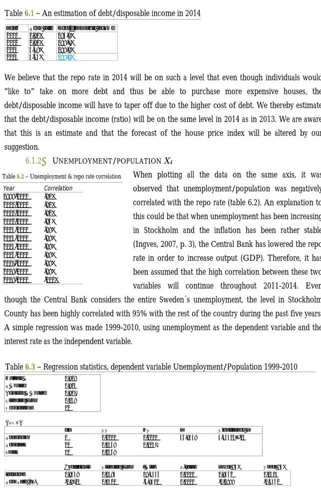
We believe that the repo rate in 2014 will be on such a level that even though individuals would “like to” take on more debt and thus be able to purchase more expensive houses, the debt/disposable income will have to taper off due to the higher cost of debt. We thereby estimate that the debt/disposable income (ratio) will be on the same level in 2014 as in 2013. We are aware that this is an estimate and that the forecast of the house price index will be altered by our suggestion.
6.1.2 UNEMPLOYMENT/POPULATION X4
When plotting all the data on the same axis, it was observed that unemployment/population was negatively correlated with the repo rate (table 6.2). An explanation to this could be that when unemployment has been increasing in Stockholm and the inflation has been rather stable (Ingves, 2007, p. 3), the Central Bank has lowered the repo rate in order to increase output (GDP). Therefore, it has been assumed that the high correlation between these two variables will continue throughout 2011-2014. Even though the Central Bank considers the entire Sweden´s unemployment, the level in Stockholm County has been highly correlated with 95% with the rest of the country during the past five years. A simple regression was made 1999-2010, using unemployment as the dependent variable and the interest rate as the independent variable.
,
Table 6.2 – Unemployment & repo rate correlation
Table 6.3 – Regression statistics, dependent variable Unemployment/Population 1999-2010 Table 6.1 – An estimation of debt/disposable income in 2014
Year Repo rate Debt/disposable income
2011 1,81% 184,8% 2012 2,81% 188,7% 2013 3,39% 189,9% 2014 3,63% 189,9% Multiple R 0,908 R Square 0,824 Adjusted R Square 0,807 Standard Error 0,068 Observations 12 ANOVA df SS MS F Significance F Regression 1 0,2200 0,2200 46,9359 4,45314E-05 Residual 10 0,0469 0,0047 Total 11 0,2668
Coefficients Standard Error t Stat P-value Lower 95% Upper 95%
Intercept 0,9439 0,0483 19,5356 0,0000 0,8362 1,0515 RepoRate (X ) -0,9725 0,1420 -6,8510 0,0000 -1,2888 -0,6562 Year Correlation 1999-2010 -91% 2000-2010 -91% 2001-2010 -92% 2002-2010 -96% 2003-2010 -99% 2004-2010 -99% 2005-2010 -99% 2006-2010 -99% 2007-2010 -99% 2008-2010 -99% 2009-2010 -100%
The slope coefficient was negative as expected. The t-value of the repo rate was statistically significant when compared to the critical value of ± 2.228 (two-tailed, = 0.05). The critical F-value for the regression is 4.96, which was lower than the actual F-value of 46.93. Thus we noted that the model was significant. The adjusted R2 for the plot is 80.7% and the overall fit of the
regression 1999-2010 is shown in graph 6.4 (dashed in light blue).
The obtained intercept and slope coefficient were used in the forecast of unemployment/population and since the repo rate already had been forecasted by the Swedish Central Bank, we could estimate the future X4. Presented in graph 6.5 are the unemployment/population (blue) and the repo rate (orange) plots with their respective forecasts. The graph clearly shows a strong relationship between the two variables.
We expects that the unemployment/population in Stockholm County will decrease to 2.0% in 2014 from 3.2% in 2010, that is, down from 65 733 to 42 473 “unlucky” individuals.
6.2
R
EPO RATE AND DEBT/
DISPOSABLE INCOME PROBABILITY INTERVALSThe prognosis reports released by the Central Bank always include high and low probability intervals. We have chosen to include the 25% probability intervals in the forecast, thus three major outcomes will be presented in the forecast. It should be noted that an infinite number of outcomes are possible within the upper and lower boundaries (75% probabilities).
6.3
C
OMBING THE RESULTSTable 6.4 presents the forecasted two independent variables which were used to forecast also the dependent variable. High and low represent 25% probability intervals prognosticated by the Central Bank. The higher probability interval means that the repo rate will be increased with more than the expected levels and the lower probability interval means that the repo rate will be kept low over the next coming years.
Graph 6.4 – Regression fit to actual X4, incl. forecast, 1993-2010 Graph 6.5 – X4 & repo rate, incl. forecast 1993-2014
0% 10% 20% 30% 40% 50% 60% 70% 80% 90% 100% 1993 1994 1995 1996 1997 1998 1999 2000 2001 2002 2003 2004 2005 2006 2007 2008 2009 2010 2011 2012 2013 2014 0% 20% 40% 60% 80% 100% 120% 140% 160% 180% 200% 1993 1994 1995 1996 1997 1998 1999 2000 2001 2002 2003 2004 2005 2006 2007 2008 2009 2010 2011 2012 2013 2014
With these forecasted values we now plot the dependent variable and the two independent variables used in the multiple regression analysis. We also plot and all the other variables included in the analysis and the repo rate (graph 6.6).
Year Debt X high Debt X Debt X low Disposable income Tax Inflation Debt/disposable income high Debt/disposable income Debt/disposable income low
2010 270 880 kr 155 694 kr
2011 277 779 kr 291 806 kr 305 804 kr 157 883 kr 30,04% 2,5% 193,7% 184,8% 175,9% 2012 284 511 kr 301 696 kr 319 255 kr 159 845 kr 30,04% 2,1% 199,7% 188,7% 178,0% 2013 283 927 kr 305 668 kr 327 024 kr 160 985 kr 30,04% 2,6% 203,1% 189,9% 176,4% 2014 285 978 kr 307 918 kr 329 386 kr 162 147 kr 30,04% 2,6% 203,1% 189,9% 176,4%
Year Unemployment/population X high Unemployment/population X Unemployment/population X low Population Repo rate high Repo rate Repo rate low
2011 2,4% 2,7% 2,8% 2 084 683 2,5% 1,8% 1,4% 2012 1,6% 2,3% 2,9% 2 114 203 4,5% 2,8% 1,2% 2013 1,1% 2,1% 3,0% 2 142 798 5,7% 3,4% 1,1% 2014 1,0% 2,0% 2,9% 2 170 576 6,1% 3,6% 1,2%
Year House Prices Y high House Prices Y House Prices Y low House Prices Y high House Prices Y House Prices Y low
2011 305,4% 318,8% 333,2% 4 071 251 kr 4 250 027 kr 4 441 942 kr 2012 319,5% 333,2% 347,3% 4 349 959 kr 4 535 959 kr 4 728 663 kr 2013 322,9% 339,5% 355,8% 4 513 930 kr 4 745 920 kr 4 973 420 kr 2014 326,4% 342,9% 358,9% 4 683 901 kr 4 919 840 kr 5 150 121 kr
Indexed from 1993 Nominal numerical terms (re-adjusted for inflation)
1993 1994 1995 1996 1997 1998 1999 2000 2001 2002 2003 2004 2005 2006 2007 2008 2009 2010 2011 2012 2013 2014
Housing prices (Y) high - 25% probability 291,2% 305,4% 319,5% 322,9% 326,4%
House prices (Y) (real terms) 100,0% 106,8% 105,3% 103,3% 115,7% 130,7% 146,8% 176,3% 196,4% 201,1% 204,3% 215,9% 228,4% 252,9% 279,5% 270,3% 274,3% 291,2% 318,8% 333,2% 339,5% 342,9%
Housing prices (Y) low - 25% probability 291,2% 333,2% 347,3% 355,8% 358,9%
Repo rate (X ) high - 25% probability 5,7% 28,3% 50,8% 64,8% 68,9%
Repo rate 100,0% 81,5% 96,8% 71,2% 46,7% 47,0% 34,5% 42,2% 45,2% 46,3% 35,8% 24,5% 19,7% 25,1% 39,3% 47,1% 7,4% 5,7% 20,6% 31,9% 38,5% 41,3%
Repo rate (X ) low - 25% probability 5,7% 16,3% 13,2% 12,5% 14,1%
Disposable income (X )(real terms) 100,0% 101,9% 100,9% 104,7% 108,0% 113,6% 120,5% 128,7% 135,5% 132,5% 128,9% 129,7% 132,8% 135,2% 138,6% 140,0% 141,2% 144,1% 146,2% 148,0% 149,0% 150,1%
Debt (X ) high - 25% probability 270,0% 276,8% 283,5% 283,0% 285,0%
Debt (X ) (real terms) 100,0% 99,0% 94,5% 102,9% 111,3% 122,0% 134,3% 148,2% 170,5% 169,4% 174,1% 188,4% 206,1% 220,5% 232,7% 237,1% 254,5% 270,0% 290,8% 300,7% 304,6% 306,9%
Debt (X ) low - 25% probability 270,0% 304,8% 318,2% 325,9% 328,3%
Unemployment/population (X ) 100,0% 95,1% 92,9% 89,5% 91,6% 71,4% 54,9% 43,8% 40,0% 48,6% 67,2% 72,3% 77,9% 73,7% 63,0% 57,6% 82,5% 88,7% 74,4% 63,4% 57,0% 54,3% Number of houses/population (X ) 100,0% 99,4% 98,9% 98,3% 97,8% 97,4% 97,0% 96,8% 97,1% 97,4% 97,6% 97,8% 97,7% 97,0% 96,3% 95,7% 94,5% 93,6% 0 0,5 1 1,5 2 2,5 3 3,5 4 1993 1994 1995 1996 1997 1998 1999 2000 2001 2002 2003 2004 2005 2006 2007 2008 2009 2010 2011 2012 2013 2014
F
O
R
E
C
A
S
T
6.4
I
NTERPRETING THE RESULTAs showed in graph 6.6, the repo rate has been prognosticated to increase over the next few years, in non-index terms the increase will be from 0.50% in 2010 (table A1.1) to 3.63% in 2014 (table 6.4). Also note that there is a 25% probability that the repo rate will be increased by more than the most probable outcome (dashed in grey). In this case, the forecast reveals that the house prices will increase in a slower pace compared to previous years. Additionally, there is also a 25% probability that the repo rate will remain at a relatively low level. In this case the house prices and leverage will continue to increase in an even higher pace than the most probable outcome (dashed in purple). Since we have assumed that the negative correlation between unemployment/population and the repo rate will continue, it has been noted that when the repo rate now is expected to increase, the unemployment/population is expected to decrease. Theoretically, we stated that the house price index is negatively correlated with the unemployment; when observing the plots in graph 6.6 we noticed the “dampening” effect when the unemployment increased during the years. We can also see that the repo rate has remained lower throughout all the years included in the analysis compared to the level in 1993, which most probably has affected the level of leverage by Swedish households and finally the house prices. The leverage has increased by much more than the disposable income and the gap between these two variables has become much larger compared to previous years. Since the leverage now has reached a level of 174% over the disposable income and is expected to increase to 189.9% in 2014, the risk for insolvencies will increase for some individual households as they might be unable to pay off their loans when the repo rate increases. The forecast reveals that the house prices and leverage will continue to increase over the next four years, but then gradually fade off when the repo rate increases. The mean market price for a house in 2014 is forecasted to be 4 919 840 kr. and when comparing to the mean market price of 3 783 000 kr. 2010, the increase is substantial. Considering the high leverage and increasing repo rate, the weak point with the statistical technique used is that it cannot foresee turning points and whether there is a price bubble or not.
According to rational expectations, the house prices presented in the graph should mirror their true values (Kindleberger & Aliber, p. 38), which means that no abnormal returns can be earned. Expectations of this altitude contradict adaptive expectations, which is a belief that abnormal returns can be achieved. Abnormal prices are often started when the individuals believe that the investment is “risk free”; this belief is grounded in the expectations that the prices will continue to increase (Case & Shiller, 2003). The survey conducted by SEB showed that more people believe in increasing house prices in April 2011 compared to March 2011. At the same time, the households do not believe that the repo rate is going to increase with the same level prognosticated by the Central Bank (Lindqvist Sjöström, 2011). In addition, the research conducted by Nordberg and
Soultanaeva (2011, p. 356) showed that the mortgage ceiling had least effect on the house prices in the Stockholm area; some of their empirical evidence can probably be described by uniqueness bias.
Mob psychology can also be a reason for the increase in house prices as everybody wants to take part of the high returns. In the beginning this behavior can be seen as rational, but when more people align, the behavior can develop excess risk taking in the form of leverage, i.e. an irrational behavior. In the graph we note the increasing leverage by households, even in times of an increasing repo rate. This phenomenon can be explained by the decreasing number of houses per person and the expectations that the positive trend on the house market will continue. In such situations individuals might think that it is “ok” to expand their debt. We also believe that there is a subconscious incentive not to increase the pace of building new houses, since it favors the existing house owners as well as the communities’ attractiveness. We believe that this sort of thinking already is in the minds of people and that they feel stressed to enter the house market before it is too late.
With the result from the multiple regression and all these facts presented, some portion of the house prices might very well be abnormal.
7
C
ONCLUSION
Conclusions with regards to the analysis carried out, fulfilling the purpose and answering the research questions of the thesis.
The purpose of this paper was to forecast the future trend of housing prices in Stockholm County 2011-2014. From the four selected macroeconomic variables, we finally chose to use two, namely the debt X1 and unemployment/population X4. It was noted that the four variables used had multicollinearity and autocorrelation issues, which has been corrected. This yields the final conclusion.
7.1
F
ULFILLING THE PURPOSEThe future trend of housing prices in Stockholm County has been forecasted to be positively sloped throughout all the years 2011-2014, but in 2011, the forecast reveals that the increase of house prices will taper off. At the end of 2011, the mean price for a house is forecasted to be 218.8% higher (real terms) compared to the level in 1993. In 2014 it is forecasted to increase to 242.9%. The forecast also reveals two more outcomes of the house price index. There is a 25% probability of a higher interest rate than prognosticated; this results in a forecasted house price index of 226.4% in 2014, thus less than the most expected outcome. In addition, there is a 25% probability of a lower interest rate than prognosticated; in this outcome, the house price index is forecasted to increase more rapidly to a 258.9% higher level compared to 1993. Nevertheless, behavioral economics reveals some insights about the trend on the housing market and that the house prices might include a portion of abnormal returns. If this would be the case, historical turning points have shown that the prices correct themselves in the long-run.