The platoon dispersion factor in Transyt for Swedish traffic conditions

ISSN 0347-6049

f V'I/meddelande f

569A

f

1988

The platoon dispersion factor in Transyt for

Swedish traffic conditions

[SS/V 0347-6049

mneeezande

The platoon dispersion factor in Transyt for

Swedish traf c conditions

Ulf Hammarstrém

VTl, Linkb'ping 1 988

VHg-UC/l

-

Statens vég- och trafikinstitut/VT/l - 581 01 Linkc ping

FOREWORD

The Swedish Road and Traffic Research Institute (VTI) has been working

since 1984L on a project commissioned by the National Road Administra-tion which is aimed at more efficient control of coordinated traffic signals. The project is divided into the following sub-projects:

o "User friendly Transyt"

0 "Automatic updating with Transyt"

Transyt is a computer program for calculating the best timing in a signal

system. The platoon dispersion factor in the Transyt program is the subject of a special study which belongs to both sub-projects mentioned

.

above.

The project has included field studies, computer calculations and

pro-gramming of the evaluation routine. The field studies and subsequent evaluation have been carried out by Leif Karlsson. Computer programm ing has been performed by Bo Karlsson.

N

P

P

P

P

W

FF

-R

EOREWORD

ABSTRACT

SUMMARY

INTRODucnON

DESCRIPTION OF THE PROBLEM

Fv iETHOD

Chosen measuring sections Measuring equipment

Measurements Method of analysis

RESULTS

Results obtained by the VTI

Results obtained by other researchers

DISCUSSION REFERENCES APPENDIXES

Appendix 1: Computer program for

estimating the platoon

dispersion factor

Appendix 2: Summary of measurements obtained by other researchers

VTIMEDDELANDE56%R

The platoon dispersion factor in Transyt for Swedish traffic conditions

by Ulf Hammarstrom

Swedish Road and Traffic Research Institute (VTI)

5-581 01 LINKOPING

ABSTRACT

The platoon dispersion factor in Transyt has been measured for Swedish traffic conditions. The values obtained indicate that the platoon

disper-sion for Swedish traffic conditions is considerably less than for foreign

conditions. The difference in platoon dispersion may be explained by

II

The platoon dispersion factor in Transyt for Swedish traffic conditions

by Ulf Hammarstrom

Swedish Road and Traffic Research Institute (VTI)

5-581 01 LINKOPING

SUMI VIARY

In calculating optimal timing of coordinated traffic signals, use is made of

a computer program named "Transyt". Transyt includes a routine for calculating platoon dispersion. Input data to the ro"tine for platoon dispersion include a platoon dispersion factor (K).

Platoon dispersion is a function of driving behaviour, which may vary both

geographically and timewise, although other conditions are similar. It is

therefore desireable to determine the platoon dispersion factor for

current Swedish conditions.

The following K-values have been measured on sections of road which

have a comparatively good geometric standard, no kerbside parking and no secondary conflicts with other road users:

0 0.26 for 1 lane 0 0.18 for 2 lanes

The default value for K applied in Transyt is 0.35, which corresponds to a greater platoon dispersion than for the sections measured in Sweden. The Swedish values recorded are clearly lower than other values found in the literature, which may be explained by the fact that the measuring 1 conditions are not exactly comparable. The term "conditions" here refers

both to those involving the environment and those relating to the method

of analysis.

In this study, traffic measurements have been carried out on sections with

a length of 100 - 205 m. Each measuring period comprised 0.5 h or about

200 cars. Video cameras were placed at the boundaries of the section

III

where measurements wereto be made. The time of each vehicle passage

was recorded at boundaries 1 and 2 and the transit time per vehicle

between the two boundaries was calculated. A mean transit time per measurement was calculated and used in estimating K. A K value was estimated for each measurement by choosing the K value giving the smallest deviation between recorded and calculated number of vehicles

per unit of time at boundary 2.

Sensitivity with regard to deviation from true mean transit time has been investigated. If, for example, the transit time entered in the platoon dispersion model is 2 % shorter than the measured mean transit time, the

value of optimal K will increase by an average of at least 200 % compared

to optimal K for mean transit time.

According to the literature, a deviation of 25 % in K-value from the true

value can lead to a loss in efficiency of 5 %, i.e. of the same order of size

as the gain in efficiency expected when using Transyt.

This account contains no conclusions as the values to be chosen for the

platoon dispersion factor. Instead, it should be regarded as a basis for

1. INTRODUCTION

Satisfactory time-schedules for controlling traffic signal systems demand

reliable input data. When calculating time-schedules, input data may

include information on how a vehicle platoon changes along a section of road. The Transyt computer program, which is designed for calculating efficient time-schedules, contains a routine for describing how the platoon dispersion changes when a queue of vehicles is studied at various points along a road. Figure 1 shows an example of a comparison of

measured and calculated platoon dispersion according to Reference 80-1.

A platoon is described at four points along a section of road. The left half of the illustration shows measured values and the right half predicted values according to Transyt.

The VTI has been working since 1984 on a project commissioned by the

National Road Administration to develop a user friendly Transyt and also to develop a method for automatic updating of time-plans. The objective of user-friendly Transyt is not limited to developing an easily used method, but also for the method to result in an improved calculation basis

and thereby more efficient time-plans. Improved calculation data also

include a correct description of platoon dispersion.

eliL

MEASURED ARRIVAL PATTERNS

'3 r

3 o

1 L J

g PREDICTED ARRIVAL PATTERNS

E 1800 f: '1 33-"??? 0 1:37.323: - 152; ":§;.'§:. _£5-5- ' 0 10 20 30 40 50 60 0 10 20 30 40 50 60 1800 E 312-? 21031 E o 1 . 0.. e o 10 20 30 4o 50 so

3

Figurel An example of measured and calculated platoon dispersion according to Reference 80 1.

2. DESCRIPTION OF THE PROBLEM

A correct description of platoon dispersion is of great significance for

coordinating traffic signals. The basic principle for platoon dispersion is

that the greater the distance from a point where a well-defined platoon

can be distinguished as such, the more dispersed the platoon will be, see

Figure l. A prerequisite for coordinating two signal installations is that

there is a systematic variation in the arrival frequency per unit of time

during a cycle.

Platoon dispersion is described and calculated in Transyt with a recursion

formula as follows:

QINU(I + IT) F x QUTUU) + (l - F) x QINU(I + IT - 1)

IT

: Integer part of (B x MT/TS)

F

= (1 + K x 1T)-l

QINU() = Number of vehicles per time increment past the

second checkpoint

I : Counter for time increment

IT = A corrected measure of the mean transit time between the first and second counting point express-ed in time increments

F = Smoothing factor

QUTU( ) = Number of vehicles per time increment past the first checkpoint

B : Transit time factor

MT = Mean transit time expressed in seconds TS : Number of seconds per time increment K : Platoon dispersion factor

The positions between which platoon dispersion is described in Transyt consist of stop lines, real or fictive, in connection with junctions. The

dispersed traffic per stop line upstream and per incoming traffic stream is

designated QINU(I+IT) in the recursion formula.

The recursion formula includes the smoothing factor F. The larger the

value of F, maximum 1, the smaller the platoon dispersion and the more

important it becomes to coordinate traffic signals. F is a function of

time, the greater the value of F and the greater the benefit of coordinating traffic signals.

The smoothing factor F is in turn a function of the corrected measure of transit time IT and platoon dispersion factor K. Increasing values of IT and K result in a lower value of F and thus reduced prospects of

coordination.

With regard to IT, the Transyt manual does not indicate whether the program uses truncation or rounding off. I-Iere, truncation has been used.

In this study, the median value of MT was 9.9 seconds. The transit time expressed in increments is corrected in Transyt with the factor B, which has been assigned a value of 0.8 by the TRRL (Transport and Road Research Laboratory) and which cannot be altered by the user of the program. No motivation for B, other than that of optimal adaptation, is

given in the Transyt manuals.

If all vehicles between two points on a section of road maintain the same speed, no platoon dispersion would occur. Platoon dispersion is an expression of the Speed distribution or transit time distribution.

The platoon dispersion factor K, upon which this study focusses, has been

assigned a value of 0.35 by the TRRL. The value of the platoon dispersion

factor is probably a function of many different variables, the principal

ones being the following:

number of lanes lane width speed limit

proportion of heavy vehicles

traffic flow

gradient

0 distance from "incoming" stop line in the form of the creation of two groups of vehicles at the junction, one group that has passed through

without stopping and one that has stopped. If the distance is small, the

group about to be stopped may still be accelerating, i.e. the situation is partly comparable with an upward gradient.

0 distance to the next stop line, together with the following: signal indication displayed

disturbance by pedestrians or by vehicles

0 parking or bus stops

0 how familiar road users are with timing of the signals, which is in turn a function of the age of the timing and the proportion of road users with knowledge of the roads in the area

0

0 road conditions

0 deviation between true transit time and transit time entered

If platoon dispersion is regarded as a function of the above points, there is

a considerable need for a special model for determining the platoon

dispersion factor in different road and street environments.

In Transyt, the platoon dispersion factor is assumedito be constant during the period covered by a calculation. However, it is probable that the platoon dispersion per link varies during the sequence, i.e. different values may be desirable for green and red signal indications respectively. Transyt has no facility for processing different platoon dispersion factors for different parts of the cycle time. The question is what value should be

used in Transyt: the green value, the red value or the mean. Normally, the

mean is used.

An important issue in determining K is whether or not to assume that MT is a correct determination of the true transit time. The problem of applying correct transit times in practical. use of Transyt should perhaps not be overemphasized since road users become familiar with timings and

for road users to be able to choose the correct speed, it must be

physically possible to achieve that particular speed. This should never be

any problem for cars, but it may be a problem for heavy vehicles. The possibility of learning a signal system is a function of the proportion of

local traffic. The importance of introducing correct speeds/transit times in Transyt thus appears greatest for signal systems on through routes. If a given transit time in a Transyt link differs comparatively greatly from the

true transit time and the K-value is relatively small, then there is a fairly

large risk that the calculated timing will only offer a small proportion of vehicles a green wave along the link, i.e. the true arrival interval may be generally unrelated to the calculated figure.

3. METHOD

3.1 Chosen measuring sections

Measurements have been made on a total of four measuring sections,

Bergsvagen, Industrigatan, Malmslattsvagen and Norrkopingsvagen. All

these sections are located in the town of Linkoping.

Measuring section on Bergsvagen in the direction towards, the town centre:

0 1 lane '

-0 speed limit 7-0 km/h

0 upward gradient O-l%

a after an isolated signalized junction i.e. drivers are not approaching any visible signals. There is a risk that the measuring section was so

close to the junction that the desired speed was not achieved o no parking and no bus stops

0 length approx. 185 m and 205 m respectively

Measuring section on Industrigatan in the direction away from the town

centre: 2 lanes speed limit 70 km/h 0 o 0 gradient 0%

0 between two coordinated signalized junctions o no parking and no bus stops

length approx. 100 m

Measuring section on Malmslattsvagen in the direction towards the town

centre:

1 lane (+1 for public transport, excluded from this study)

speed limit 50 km/h 0

o

0 gradient 0%

0 between two coordinated signalized junctions o no parking and no bus stops

0 length approx. 70 m and 140 m respectively

Measuring section on Norrkopingsvagen in the direction towards the town

centre:

a 2 lanes

0 speed limit 70 km/h

0 gradient. 0%

0 after an isolated signalized junction and without any visible signalsin

the direction of travel

no parking and no bus stops

length approx. 120 m and 140 m respectively

The measuring sections have in every case been located at relatively large

distances upstream of the junction, i.e. an attempt has been made to minimize the influence of disturbances from the next junction.

3.2 . Measuring equipment

Traffic is recorded in parallel at two points. The parameter measured is the number of vehicle passages per time interval at each checkpoint. In

addition, the mean transit time between the points is recorded. Simple tape recorders are used during the first measuring session. The tape recorders were started and synchronized with regard to time. An observer

was placed at each checkpoint and described each passing vehicle on his tape recorder. One problem with this method was keeping pace with the traffic, since the time between vehicles was very short. In the extreme case, two vehicles could pass the observer at the same time. The other

problem was that the tape recorders had unstable speed, resulting in a

different time for recording compared to playback. A decision was therefore made to use video cameras, which eliminated both these problems.

3.3 Measurements

A total of 9 measurements were distributed among the specified

measuring sections as follows:

Bergsvagen, 3 measurements Industrigatan, 1 measurement Malmslattsvagen, 3 measurements

Norrkopingsvagen, 2 measurements

The number of vehicles recorded was as follows:

Bergsvagen, 223, 226, 224

Industrigatan 134L

Malmslattsvagen, 200, 267, 202

Norrkopingsvagen, 163, ll9

Each measurement occupied 30 minutes.

Note that the traffic flow on the sections with 1 lane was considerably

greater than the flow on the sections with 2_lanes.

3.4 Method of analysis

The number of observations has been evaluated per time increment I. The

length of an increment, T5, was set at 2 seconds. A data file with the following record description was created for each measuring section and

measurement:

0 time increment no _

o no. of vehicle passages at the first checkpoint during the time increment

o no. of vehicle passages at the second checkpoint during the time

increment

The mean transit time, between the two points, MT, has been calculated

for each measurement. An estimate of the K value sought has been

obtained with a computer program as described in Appendix 1. The aim of the program is to permit calculation of the K-value giving the smallest difference between calculated and observed platoon profile at checkpoint

2.

The precision with which MT is specified is significant for the K-value obtained. The more precise MT becomes, the smaller the deviation between estimated and measured arrival time at the stop line. In this study, MT has been estimated with maximum precision by recording the

transit time for each vehicle passing along the measuring section. An

important question in comparing the K-values obtained here with those mentioned in the literature is the way in which MT has been allocated

values. This is not described in the literature references.

The significance of correct MT has been analyzed by multiplying measured values by 0.75 and 1.25 respectively.

10

4. RESULTS

4.1 Results obtained by the VTI

\_

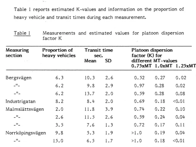
Table 1 reports estimated K-values and information on the proportion of heavy vehicle and transit times during each measurement.

Table 1 Measurements and estimated values for platoon dispersion factor K

Measuring Proportion of Transit time Platoon dispersion section heavy vehicles sec. factor (K) for

v ~ Mean SD different MT-values

O . 75XMT l . OxMT l . 25XMT Bergsvagen 6.3 10.3 2.6 0.52 0.27 0.02 -"- 6.2 9.8 2.9 0.97 0.28 0.02 -"- 6.2 13.7 2.0 0.59 0.28 0.08 Industrigatan 8. 2 8. 4 2. 0 0. 69 0.18 <0.01 Malmslattsvagen 2. 0 11. 8 3. 9' 0. 74 0. 22 0.10 -"- 2.6 11.5 2.6 0.59 0.24 0.04 -"- 3.5- 7.6 1.3 0.72 0.17 0.11 Norrkopingsvéigen 9. 8 5. 3 l. 9 >1. 0. 19 - 0.04 -"- 15.0 6.5 1.7 >1.0 0.18 <0.01

Table 1 shows that K is sensitive to the magnitude of MT and that K then decreases when the difference, including sign, between applied MT and

true MT increases.

Since K is decreasing as a function of MT, the probability increases that

the values estimated for measured MT values can represent the K values that should be applied in practice. If instead, the estimated K-values had

been minimum values, larger K values than those estimated should be

used in practical applications.

The material in Table 1 is too limited for a model of K to be developed. If

calculation of the mean is performed with regard to K for 1.0 x MT within groups with the same number of lanes, the following results are

obtained:

0 for 1 lanes, K = 0.26 o for 2 lanes, K = 0.18

11

Note that the load was considerably higher for measuring sections with 1

lane than for those with 2 lanes.

4.2 Results obtained by other researchers

Reference 87-1 describes both a literature study and results from direct measurements of platoon dispersion. The reference includes a sensitivity

analysis of B and K. B and K are multiplied by 0.75 and 1.25 respectively. Optimal timings have been calculated for all four combinations and have been used to calculate P1 with B and K multiplied by l. The maximum

deviation between PI for any of the four combinations and PI calculated

for an optimum timing with uncorrected B and K was approximately 5%. According to the literature study in the above reference, estimates of K

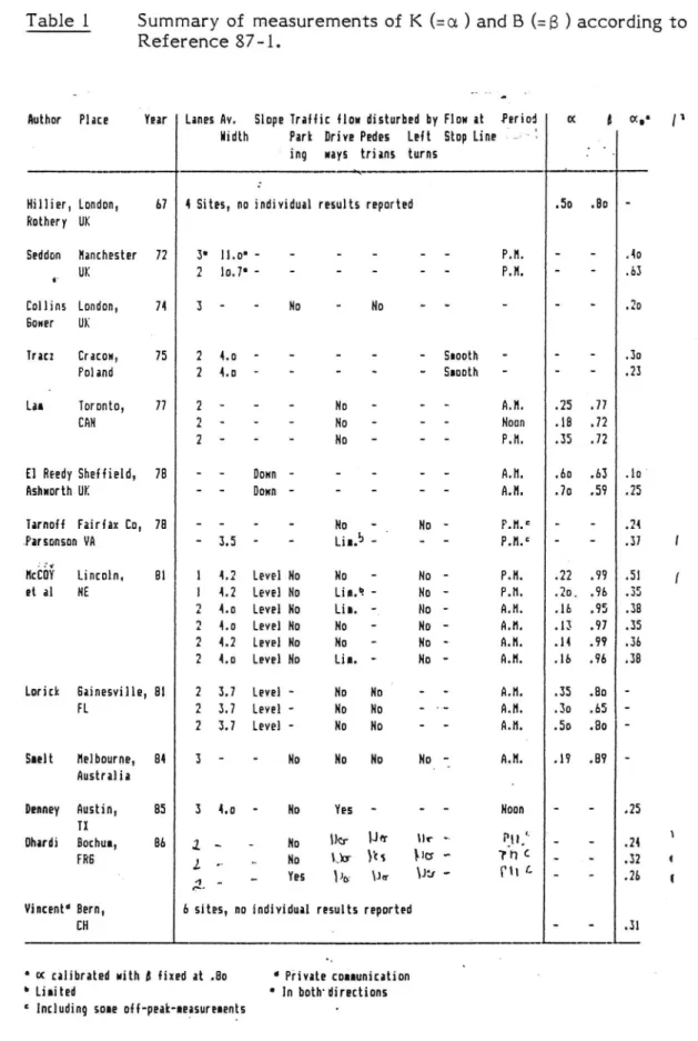
have been made since the end of the 605 to the present time, see Appendix 2. The same Appendix also contains measurements according to

Reference 87 - l .

The field study of K, described in Reference 87 1 , was intended to relate

K to the following variables: number of lanes, gradient parking, pedest-l

rians and traffic situation upstream of the stop line. The mean of all the

estimates of K was 0.37, as against the default value 0.35 in Transyt. The

dispersion in the material is comparatively large, from K = 0.01 to K =

0.87.

Road and street design is considered to be of great significance for K. In well-designed layouts, K-values of around 0.20-0.25 are not unrealistic.

According to a statistical analysis in Reference 87-1, only the following variables may be said to have a definite effect on K:

0 Number of lanes: - one lane, K = 0A6 - two lanes, K : 0.29

o -Occurrence of conflicts with pedestrians: with, K = 0.53

without, K = 0.23

12

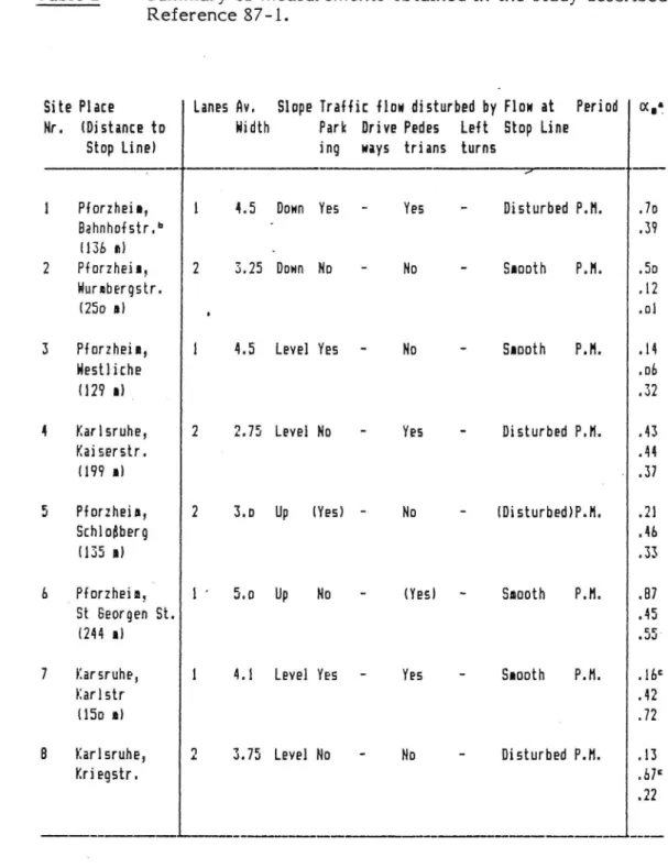
No data regarding K-values for combinations of variables have been

sUppiied in Reference 87-1, but these could be estimated since all observations of K have been documented.

l3

5. DISCUSSION

Measured K-values in this study are considerably smaller than those normally stated in the literature. The mean of the K-values recorded is estimated at 0.22, while Reference 87-1 states 0.37 as mean. One explanation may be that the standard of the measuring sections in this study is higher than the standard of the sections studied in the literature.

For example, Reference 87-1 states that K may be in the range 0.20 0.25 for a high standard.

The K value for 1 lane is considerably greater than for 2 lanes, both in

this study and in Reference 87-1. However, the difference in K between

the two studies is comparatively large.

One reason for the Swedish K-values being smaller than those obtained in other countries may be the location of the measuring sections. These have

systematically been chosen so that the effect of disturbances downstream is as small as possible. Another reason may be in the way the transit time

MT has been allocated values. In this study, a mean for each measuring

section has been estimated by recording transit time per passing vehicle.

The error in MT in the foreign studies is at least as great as in this study.

If it is assumed that the K-values obtained in this study are correct, a problem of method occurs when using Transyt. This is because MT will never be known with such great precision as in this study.

In view of the above, a model for calculating K-values should not be limited to calculating K-values as a function of environment, but should

also take into account the uncertainty in MT.

1

!-REFERENCES

80-1

87-1

Vincent, R.A., Mitchell, AJ. and Robertson, D.

User Guide to TRANSYT Version 8. TRRL Laboratory Report 888.

Transport and Road Research Laboratory, Crowthorne,

Berkshire.

Axhausen, K.W. and Koriing, H-G.

Some Measurements of Robertson's Platoon Dispersion Factor.

66th Annual Meeting of the Transportation Research Board, Washington. January 1987.

Appendix 1

Page 1(1)

Computer program for estimating platoon dispersion factor.

C 860814 10 20 30 PROGRAM KOLONN , REAL MT,K,QUTU(5000),QINU(5000),QINB(5000) CHARACTER*32 INFIL LOGICAL EOF WRITE(*,'(A,A)') $',' GE INFIL :' READ(*, (A)')INFIL

OPEN(UNIT=5,FILEzINFIL,ACCESS= SEQUENTIAL ,STATUS-'OLD)

OPEN(UNIT-6,FILE-'UT1.DAT',ACCESS-'SEQUENTIAL',STATUS- OLD') OPEN(UNIT=7,FILE= UT2.DAT',ACCESS= SEQUENTIAL',STATusa'OLD') EOF=.FALSE. TS=2. WRITE(*,'(A,A) ) ${,' GE MT:' READ(*,*)MT IT=INT(0.8*MT/TS) IMWRITE(*,'(A,A)')'$',' GE KSTART,KSLUT,KSTEG : READ(*,*)KSTART,KSLUT,KSTEG DO 1-1.4750 READ(5,*,END=S)IIN,A,B WRITE(*,*)IIN,A,B QUTU(IIN)=A QINU(IIN)=B N=IIN END DO CONTINUE DO K-KSTART,KSLUT,KSTEG DO 121,4750 QINB(I)-O. END DO DELTA-0. F-(1+((IT*K)/100.))**(-l) I-O CONTINUE I-I+1

IF(I.GT.4750)STOP ' F\R MlNGA VIRDEN'

CONTINUE -QINB(I+IT)=F*QUTU(I)+(l.-F)*QINB(I+IT-1) WRITE(6,'(IS,F10.5)')I*IT,QINB(I+IT) WRITE(6, (IS,F10.5)')(I+1)*IT,QINB(I+IT) WRITE(7,'(IS,F10.5)')I*IT,QINU(I+IT) WRITE(7,'(IS,FLO.5)')(I+l)*IT,QINU(I+IT) DELTA-DELTA+ABS(QINB(I+IT)-QINU(I+IT)) IF(I.LE.N)GO TO 10 IF(QINB(I+IT).LT.0.2)GO TO 30 I-I+1

IF(I.GT.4750)STOP F\R MlNGA ITERATIONER'

GO TO 20

CONTINUE

WRITE(*,'(A,F7.2,F15.8) ) DELTA/I : ,K,DELTA/I

END DO

CLOSE(UNIT-5) END '

Appendix 2 Page 1(2)

Table 1

Summary of measurements of K (:01 ) and B (:8 ) according to

Author Place Year Lanes Av. Slope lraliic 410v disturbed by Flow at Period (x 3 01,- [1 Hidth Park Drive Pedes Left Stop Line »ra'~1

' ing uays trians turns

Hillier, London, 67 4 Sites, no individual results reported .50 .80 -Rothery UK

Seddon Manchester 72 3' 11.0' - - - 8.8. - - .40

._ UK 2 10.7' - - - P.H. - - .63

Collins London, 74 3 - - No - N0 - - - .20

Boner UK

Iracz Cracou, 75 4.0 - - - Snooth - - - .30 Poland 2 4.0 - - - Snooth - - ~ .23

La Twmnm n 2 - - - No . - - mm 15 .n

CAN 2 - - - No - - - Noon .18 .72

2 - - - No - - - 8.8. .35 .72 El Reedy Sheffield, 78 - - Donn - - - 9.". .60 .63 .lo' Ashuorth UK - Donn - - - A.H. .70 .59 .25 Tarnoil Fairlax Co, 78 - - - - N0 - . No - P.H.= - - 24 .Parsonson VA - 3.5 - - Li|.5 - - - P.h. - - .37 I

8:88? Lincoln. 81 1 4.2 Level No No - N0 - P.H. .22 .99 .51 I et a1 NE 1 4.2 Level N0 Lia.9 - No - 8.8. .20. .96 .35

2 4.0 Level No Lia. -_ No - A.H. .16 .95 .38

2 4.0 Level No No - N0 - 8. . .13 .97 .35

2 4.2 Level No No - N0 - 9.". .14 .99 .36

2 4.0 Level No Lil. - N0 - A.H. .16 .96 .38 Lorick 8ainesville, 81 2 3.7 Level - No No ' - - A.h. .35 .80

-FL 2 3.7 Level - No No - '- A.H. .30 .65 -2 3.7 Level - N0 N0 - - A.h. .50 .80 -Slelt Melbourne, 84 3 - - No No No No 1 A.H. .19 .89

-Australia '

Denney Austin, 85 3 4.0 - No Yes - - - Noon - - .25

TX ,

0mm 80chun,

86

.2 -

-

No

Ucr

'f

"r "

1 :

-

-

.24

F88 l , .. No Liar Y s 1 5 * T C - - .32 i

4 - _ 5 in u. \k:» 181 - - as .

Vincentd Bern, 6 sites, no individual results reported

CH - - .31

(X calibrated with 8 fixed at .30

' Linited

Including SOIE cit-peat-eeasurenents

VTIMEDDELANDE56$R

Private con-unication

Appendix 2

Page 2(2)

Table 2 Summary of measurements obtained in the study described in Reference 87-1.

Site Place Lanes Av. Slope lralfic (lou disturbed by Flow at Period (x.e Nr. (Distance to Hidth Park Drive Pedes Left Stop Line

Stop Line) ing ways trians turns

1 Plorzheio, l 4.5 Down Yes - Yes - Disturbed P.H. .7o

Bahnhoistr.b ' .39

(136 n) .

2 Pforzheil, 2 3.25 Donn No - No - Snooth P.H. .5o

Hurnbergstr. .12

(250 I1 , .ol

3 Pforzheia, 1 4.5 Level Yes - No - Soooth P.H. .14

Hestliche .06

(129 I17 .3

4 Karlsruhe, 2 2.75 Level No - Yes - Disturbed P.H. .43

Kaiserstr. .44

(199 a1 . . .37

5 Plorzheia, 2 3.0 Up (Yes) - No - (Disturbele.H. .2

Schlodberg .i6

(135 a) .33

6 _ Pforzheio,i l ' 5.0 Up No - (Yesl - Soooth P.H. 87

St Beorgen St. 45

(244 I1 55~

7 Karsruhe, 1 4.1 Level Yes - Yes - Slooth P.H. .16

Karlstr . 2

(150 :1 x .72

8 Karlsruhe, 2 3.75 Level No - No - Disturbed P.H. .13

Kriegstr. .67

1

(X calibrated with 8 fixed at .80

Only two intervals due to equipoent naltunctioninq

Excluded iron the analysis