U.U.D.M. Project Report 2011:29
Examensarbete i matematik, 30 hp
Handledare och examinator: Takis Konstantopoulos November 2011
Department of Mathematics
Brownian Motions and Scaling Limits of
Random Trees
I would like to dedicate this thesis to my brother, Rasta, who is more than a brother to me. Guiding me through my studies and
Abstract
Brownian motions as continuous time stochastic processes are scal-ing limit of different mathematical objects in distribution. When a polygon triangulation tends to a triangulation of the circle, a simple random walk tends to normalized Brownian motion in distribution. A similar thing can be argued for plane, real and labeled trees. The aim of this thesis is to define and check the random triangulation of the circle in more details and find the scaling limit and distribution of random trees above.
Contents
Contents iii List of Figures v List of Tables vi 1 Introduction 1 2 Catalan Numbers 2 2.1 A Brief History . . . 22.2 Isomorphism Between S1, S2 and S3. . . 4
2.3 The Values of Cn . . . 6
2.4 Some Examples . . . 9
3 Limit of Polygon Triangulation 11 3.1 Random Triangulation of the Circle . . . 11
3.1.1 Hausdorff content and dimension . . . 12
3.1.2 Two Examples of Different Triangulations . . . 13
3.2 Continuous Functions and Triangulations of the Circle . . . 14
3.3 Walks, Trees and Triangulations of n-gons . . . 15
3.4 Brownian Motions . . . 19
3.5 Random Triangulation of the Circle, Revisited . . . 20
3.5.1 Zero Set of Brownian Motion . . . 20
CONTENTS
4 Discrete Trees 25
4.1 Dyck Path and Contour Function . . . 25
4.2 Discrete Trees . . . 27
4.2.1 Plane Trees . . . 27
4.2.2 Galton-Watson Trees . . . 29
4.3 The Contour Function in the Geometric Case . . . 32
4.4 Brownian Excursions . . . 34
4.4.1 Local Time Process and Excursion Space . . . 34
4.4.2 The Itˆo Excursion Measure . . . 36
4.5 Convergence of Contour Functions Towards Brownian Excursions 40 5 Real and Labeled Trees 51 5.1 Real Trees . . . 51
5.1.1 Definition . . . 51
5.1.2 Coding . . . 53
5.1.3 Convergence of Real Tree Towards CRT . . . 56
5.2 Labeled Trees . . . 58
5.2.1 Brownian Snakes . . . 59
5.2.2 Convergence of Labeled Tree Towards Brownian Snake . . 62
List of Figures
2.1 Euler’s polygon triangulation problem. . . 3
2.2 The process of getting a polygon’s triangulation from a well-formed sequence of parentheses. . . 6
2.3 A valid sequence of parenthesis with 5 letters driven from a hexagon triangulation. . . 7
2.4 A Simple Random Walk with 2n “ 10 Walks. . . 9
2.5 Different ways of how 2n “ 6 people around a table can handshake without crossing each other hands. . . 9
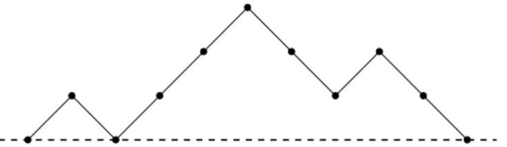
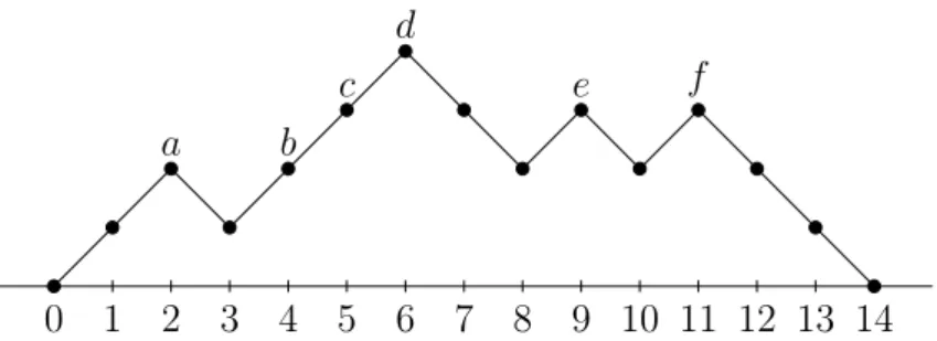
3.1 A Positive Walk with 2n “ 14 Walks. . . 16
3.2 A Plane Rooted (and Ordered) Tree with n ´ 1 “ 6 Edges. . . 16
3.3 A Binary Tree with n ´ 1 “ 6 Nodes. . . 16
3.4 A Triangulation of the Octagon. . . 17
4.1 Traversing a plane tree and its nodes’ sequences. . . 28
4.2 Contour function of the plane tree in Figure 4.1. . . 29
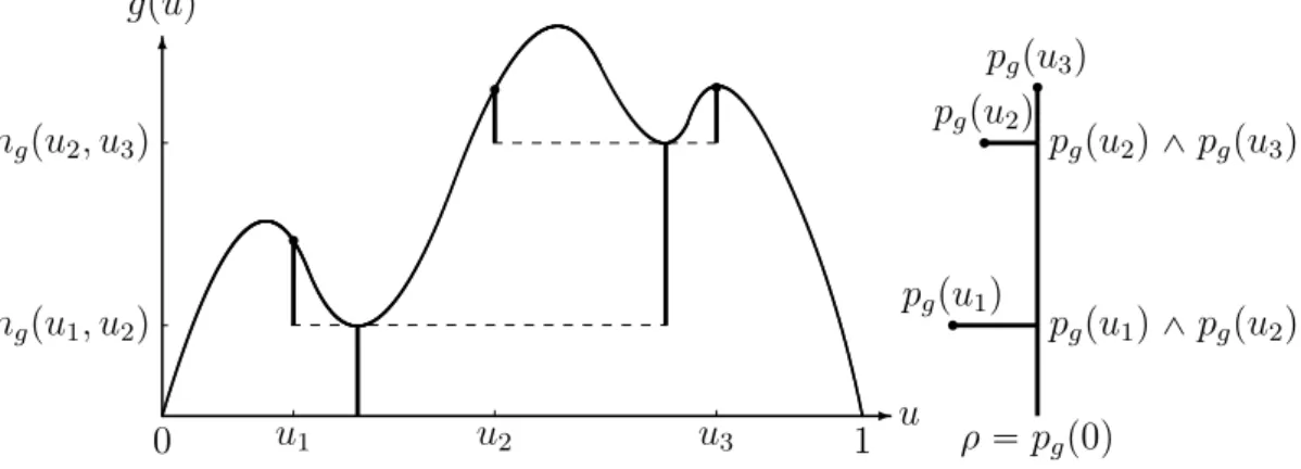
5.1 Real Tree Coded by Three Points of a Continuous Function. . . . 55
5.2 Real Tree Coded by a Continuous Function with Three Local Max-imum Points. . . 56
List of Tables
2.1 The first smallest well-formed sequences of parentheses. . . 4
Chapter 1
Introduction
This thesis is mainly based on an article[2] by David Aldous and some notes[12]
by Jean-Fran¸cois Le Gall.
We will start by discussing Catalan numbers, one of the most famous and frequently occurring sequences in Combinatorics. There exist many different examples where Catalan numbers appear when we try to count a set. Among these sets, we check three sets more in depth and use its results later.
In Chapter 3, we will state several basis definitions for the rest of the the-sis such as Hausdorff dimension and Brownian motions. We show that how the random triangulation of the circle can be encoded by normalized Brownian ex-cursions.
In the other two Chapters we will discuss about different classes of discrete trees, like plane and labeled trees and also real trees and their scaling limits will be driven.
In this thesis it has been tried to provide the proof of every statement we claim. In many cases we provided proofs if there were no proofs available in two text mentioned above and also in several cases, although a proof was provided, it has been tried to present a new proof.
Chapter 2
Catalan Numbers
Amongst the set of infinite sequences of positive integers we can mention some simple and obvious series like doubling series (1, 2, 4, 8, 16, ...) or the squares (1, 4, 9, 16, 25, ...) or some others that a few mathematicians would fail to rec-ognize like the Fibonacci numbers (1, 1, 2, 3, 5, 8, ...) or the triangular numbers (1, 3, 6, 10, 15, 21, ...). In case of an unfamiliar sequence, however, we may have to spend an enormous amount of time to find a recursive or non-recursive formula that generates the sequence[13].
When someone encounters an infinite sequence of positive integers, a pos-sible way is to look it up in A Handbook of Integer Sequences[20]. In that handbook at the top of the page 71, the 557-th sequence is the sequence that we will talk about it in this chapter, the sequence of the Catalan numbers: 1, 2, 5, 14, 42, 132, 429, 1430, ....
2.1
A Brief History
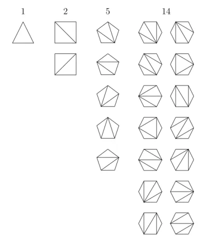
Around 1751, Leonard Euler found the Catalan numbers[15] after asking him-self: In how many ways can we divide a fixed convex polygon into triangles by drawing diagonals that do not intersect[13]? Denote the set of different polygon
triangulations by S1. The first few examples can be seen in Figure2.1.
Let us suggest a question whose solution generates the sequence of Catalan numbers too. What are the number of well-formed sequences of parentheses?
1 2 5 14
Figure 2.1: Euler’s polygon triangulation problem.
”Well-formed” means that each open parenthesis has a matching closed paren-thesis. For example amongst different sequences of n “ 3 pair of open and closed parentheses, ”()(())” is formed while ”(()))(” is not. Denote the set of well-formed sequences by S2. Look at Table 2.1 for the smallest examples of such
sequences.
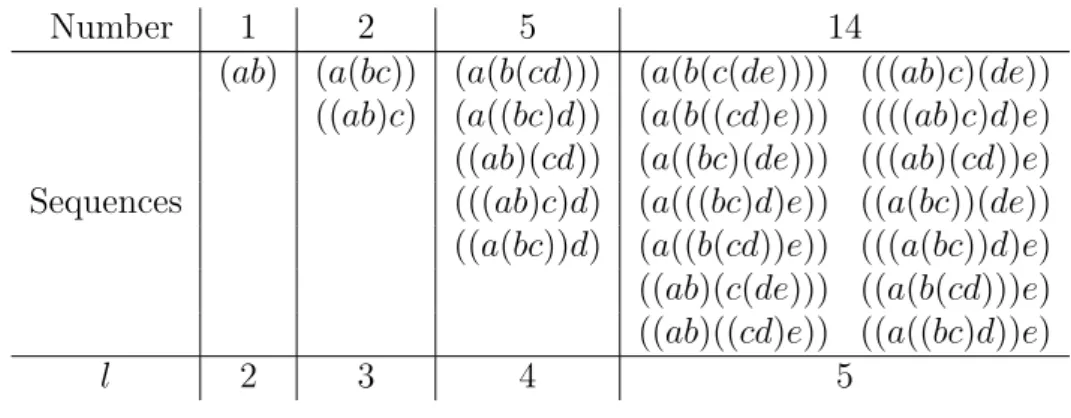
Now let us define the ”valid” sequences of parentheses with l letters as below. Suppose that we have a chain of l letters in a fixed order. We want to add l ´1 pairs of parentheses so that each pair of matched parentheses contain exactly two ”parts”. These parts can be two adjacent letters, a letter and an adjacent parenthetical grouping or two adjacent parenthetical groupings. We call these sequences valid sequences of parentheses with l letters and denote its set by S3.
The examples of such sequences of parentheses with 2, 3, 4 and 5 letters are shown in Table 2.2.
Table 2.1: The first smallest well-formed sequences of parentheses. Number 1 2 5 14 () (()) ((())) (((()))) ()()(()) ()() (()()) ((()())) ()()()() ()(()) (()(())) ()(())() Sequences ()()() (()()()) (())(()) (())() ((())()) (())()() ()((())) ((()))() ()(()()) (()())() n 1 2 3 4
Table 2.2: Examples of valid sequences of parentheses with 2, 3, 4 and 5 letters.
Number 1 2 5 14
pabq papbcqq papbpcdqqq papbpcpdeqqqq pppabqcqpdeqq ppabqcq pappbcqdqq papbppcdqeqqq ppppabqcqdqeq ppabqpcdqq pappbcqpdeqqq pppabqpcdqqeq Sequences pppabqcqdq papppbcqdqeqq ppapbcqqpdeqq ppapbcqqdq pappbpcdqqeqq pppapbcqqdqeq ppabqpcpdeqqq ppapbpcdqqqeq ppabqppcdqeqq ppappbcqdqqeq
l 2 3 4 5
In 1838, Belgian mathematician Eugene C. Catalan discovered Catalan num-bers while studying valid sequences of parentheses with l letters.
2.2
Isomorphism Between S
1, S
2and S
3.
Proposition 2.1. There is an injection from S3 to S2.
Proof. [6] Let us define an injection from the set of well-formed sequences of n pair of parentheses to the set of valid sequences of parentheses with l “ n ` 1 letters with a simple example. Suppose that we have a sequence of parentheses with l “ 5 letters, like ppabqpcpdeqqq. First put a dot between 2 parts of each pair of matched parentheses and get the sequence ppa.bq.pc.pd.eqqq. Now delete all
open parentheses and letters and get .q...qqq. Finally put open parentheses instead of each of the dots and get pqpppqqq. It is easy to see that we get a well-formed sequence.
The valid sequences in Table 2.2 are arranged in the same order as their corresponded well-formed sequences in Table 2.1.
Proposition 2.2. There is an injection from S2 to S1.
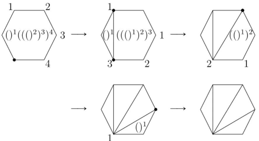
Proof. We define an injection from well-formed sequence of parentheses with n pair of parentheses to the triangulation of polygons with n ` 2 sides.
Suppose that we have pqpppqqq (a well-formed sequence with n “ 4 pair of parentheses). Start from a corresponded regular polygon which is a hexagon in our example. Set the base node the lower left node. Starting from 1, assign numbers to other nodes clockwise from the second node after the base node. Also assign numbers to the closed parentheses in the sequence from left to right. Consider the assigned number of the matched close parenthesis of the first open parenthesis.
If it is between 1 and n ´ 1, then draw a diagonal between the base node and the node with the same assigned number. By this diagonal the original polygon will be divided into 2 polygons. For the first polygon, base node remains the same. For the second polygon make the other node (the other end of the diagonal) the base node. Also divide the sequence to 2 subsequences, the first subsequence starts from the first parenthesis to the matched closed parenthesis (with the assigned number) and the other subsequence the rest of the sequence. Assign them respectively to the new and old polygons and do the same procedure for them by induction.
If the matched close parenthesis is the n-th closed parenthesis, then draw a diagonal between the nodes to the left and the right of the base node, make the next node of base node (clockwise) the base node of the new polygon. Remove the first and last parentheses from the original sequence and do the same procedure by induction for the new polygon and with the new sequence.
The basis for the induction step is of course the single pair of parenthesis which is equivalent to a triangle itself. For clarification, look at the Figure 2.2. The sequences in Table 2.1 are arranged in the same order as their corresponded
polygon triangulations in Figure 2.1. 1 2 3 4 pq1pppq2q3q4 ÝÑ 1 1 2 3 pq1pppq1q2q3 ÝÑ 1 2 ppq1q2 ÝÑ 1 pq1 ÝÑ
Figure 2.2: The process of getting a polygon’s triangulation from a well-formed sequence of parentheses.
Proposition 2.3. There is an injection from S1 to S3.
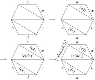
Proof. [13] In 1961, H. G. Forder showed a simple way to prove a one-on-one
correspondence between the triangulated polygons with n sides and the valid sequences of parentheses with l “ n ´ 1 letters. Let us describe the injection part of it with a simple example on a hexagon.
Except the base side, label the other sides by letters a, b, c, d, e. Each diagonal spanning the the adjacent sides is labeled with the letters of those side in paren-theses. The other diagonals are then labeled in similar fashion by combining the labels on the other two sides of the triangle. The base is labeled last. Look at Figure 2.3.
Propositions 2.1, 2.2 and 2.3 show that these sets are isomorphic. In fact a lot of other seemingly unrelated sets are isomorphic to Si’s which we will give a
few examples in Section 2.4.
2.3
The Values of C
na b c d e ÝÑ a b c d e pab q pde q ÝÑ a b c d e pab q pcpdeqq pde q ÝÑ a b c d e ppab qpcp deqqq pab q pcpdeqq pde q
Figure 2.3: A valid sequence of parenthesis with 5 letters driven from a hexagon triangulation.
For getting more simpler recursive formulas, usually they add a ”1” to the first of the sequences. If we do that with the sequence of Catalan numbers, we get the sequence (1, 1, 2, 5, 14, 42, 132, 429, ...). Put C0 “ 1, C1 “ 1, C2 “ 2, C3 “
5, C4 “ 14, ....
Consider the polygon triangulation problem. Let us try to count the number of different triangulations of a polygon with n ą 3 sides recursively. The first diagonal can be drawn between any two nodes with at least one node between them. This diagonal will divide the polygon into two smaller polygons one with k ` 1 sides and the other with n ´ k ` 1 sides where 1 ă k ă n ´ 1. Each of these new polygons can be triangulated independently. Also easily we can guess than the number of different triangulations of a polygon with n sides is equal to Cn´2,
then get the following recursive formula.
Cn “ n´1
ÿ
i“0
CiCn´i´1. (2.1)
with n sides by Tn, Euler, using an inductive argument that he described as ”quite
laborious” established that[15]
Tn “ 2 ˆ 6 ˆ 10 ˆ ¨ ¨ ¨ ˆ p4n ´ 10q pn ´ 1q! , where n ě 3. Also Tn“ Cn´2, so Tn`2“ Cn “ 2 ˆ 6 ˆ 10 ˆ ¨ ¨ ¨ ˆ p4n ´ 2q pn ` 1q! “ 4n ´ 2 n ` 1 ˆ 2 ˆ 6 ˆ 10 ˆ ¨ ¨ ¨ ˆ p4n ´ 6q n! “ 4n ´ 2 n ` 1 Tn`1; and now we conclude that
Cn“
4n ´ 2
n ` 1 Cn´1.. (2.2) From recursive equation 2.2, we can derive an explicit formula for Catalan numbers: Cn“ 4n ´ 2 n ` 1 Cn´1 “ p4n ´ 2qp4n ´ 6q pn ` 1qn Cn´2 .. . “ p4n ´ 2qp4n ´ 6q ˆ ¨ ¨ ¨ ˆ 6 ˆ 2 pn ` 1qn ˆ ¨ ¨ ¨ ˆ 3 ˆ 2 C0 “ p2n ´ 1qp2n ´ 3q ˆ ¨ ¨ ¨ ˆ 3 ˆ 1 pn ` 1q! ˆ 2 n “ p2nq! ˆ 2 n pn ` 1q! ˆ 2nˆ n! “ p2nq! pn ` 1q!n!,
and it means that Cn “ 1 n ` 1 ˆ2n n ˙ . (2.3)
So Catalan numbers can be defined by any recursive formulas in (2.1), (2.2) or the explicit formula in (2.3).
2.4
Some Examples
Here let us present a few problems[6] which introduces sets which are isomorphic
to each other and also to sets in Section 2.2.
Example 2.1 (Simple Random Walks). Consider the random walks which con-sists of n up-walks and n down-walks in such a way that we never go below the horizontal line (see Figure 2.4).
Figure 2.4: A Simple Random Walk with 2n “ 10 Walks.
The number of these random walks are equal to Cn.
Example 2.2 (Hands Across a Table[6]). If 2n people are seated around a circular table, in how many ways can all of them simultaneously shake hands with another person such that none of their arms cross each other? To see the all possible ways when n “ 3 look at the Figure 2.5.
Figure 2.5: Different ways of how 2n “ 6 people around a table can handshake without crossing each other hands.
The number of different handshaking with 2n people around table is equal to Cn.
Example 2.3 (Plane Rooted Trees). The set of rooted trees with n edge in which a specific node is root is also isomorphic to the sets defined above.
The number of rooted trees with n edges is equal to Cn.
Example 2.4 (Rooted Binary Trees). The number of rooted binary trees with n internal node (none leaf) which each nod is either a leaf or an internal node with exactly two children also generate the sequence of Catalan numbers.
The number of rooted binary trees with n internal node is equal to Cn.
There are a lot of other examples which produce the sequence of Catalan numbers. In 1971 Henry W. Gould, a mathematician at West Virginia University, privately issued a bibliography of 243 references on Catalan numbers. In 1976 he increased the number of references to 450[13]. In many cases people were not aware that they were dealing with the sequence of Catalan numbers!
In next two chapters, we will talk about the polygon triangulation and plane trees and their limits more in depth.
Chapter 3
Limit of Polygon Triangulation
In Chapter2we saw that the number of different triangulation of a polygon with n sides is equal to the pn ´ 2q-th Catalan number,
Cn´2 “ 1 n ´ 1 ˆ2pn ´ 2q n ´ 2 ˙ .
In this chapter we will discuss in more depth about the set of different trian-gulations of a polygon and its limit when n Ñ 8.
3.1
Random Triangulation of the Circle
When n Ñ 8, a regular polygon with n sides will converge to a circle; so we can consider that it is a triangulation of a circle! Based on this convergence, a random triangulation of a regular polygon with n sides when n Ñ 8, can be considered as a random triangulation of the circle. We consider the definition below for a triangulation of the circle.
Definition 3.1. A triangulation of the circle is a closed subset of the closed disc whose complements is a disjoint union of open triangles with vertices on the circumference of the circle.[2]
The triangulations defined as above are exactly the possible limits of triangu-lations of n-gons. Before talking more about different triangutriangu-lations, let us define the Hausdorff content and dimension.
3.1.1
Hausdorff content and dimension
Definition 3.2. d-dimensional Hausdorff content of S is defined by
CHdpSq :“ inf #
ÿ
i
rdi : there is a cover of S by balls with radii ri ą 0
+ ,
where S is a subset of a metric space X and d P r0, 8q.
Suppose that X Ă Rn and and λ ą 0 then it is easy to see that[16]
CHdpλXq “ λdCHdpXq. (3.1)
For proving that, suppose that a covering C of X gives the infimum of the set above, řirid which is equal to CHd, then if we replace each ball in C with a ball λ times bigger, the new sum will be ř
ipλriq d “řiλdrid“ λd ř ir d i “ λdCHd. It proves that Cd
HpλXq ď λdCHdpXq. With a similar argument we can prove that
Cd
HpXq ď 1
λdCHdpλXq; and together we conclude (3.1).
Definition 3.3. Hausdorff dimension of X is defined by
dimHpXq :“ inf d ě 0 : CHdpXq “ 0( .
With the definition of Hausdorff dimension, we can easily observe that[10]
CHdpXq “ #
8 if 0 ď d ă dimHpXq
0 if d ą dimHpXq
. (3.2)
But when d “ dimHpXq, CHdpXq is not determined. In fact it can be either 0 or
infinity or may take any value between 0 and infinity.
In general finding the Hausdorff dimension of a space directly is rather a hard work! The calculating is usually done by using some basic techniques that are available for dimension calculations. For example the equation 3.1 can be used sometimes to establish an upper or a lower bound for the Hausdorff dimension.
Let us explain a simple example in which we calculate the Hausdorff dimension directly. We prove that the Hausdorff dimension of the interval r0, 1s is 1.
We define different coverings of the interval r0, 1s for each k “ 1, 2, ..., and denote them by Ck as follows. Ck is a covering consists of k segments rki,i`1k s for
each i “ 0, 1, ..., k ´ 1. Now let us calculate řiridfor a specific k and an arbitrary d: ÿ i rdi “ k ÿ i“0 p1 kq d “ k kd “ k 1´d ,
so when k Ñ 8, the sum goes to 0 if d ą 1 and goes to infinity if d ă 1 and according to (3.2) we conclude that the Hausdorff dimension of the interval r0, 1s is 1.
Other examples can be a countable set, circle and Rn which have Hausdorff
dimension respectively 0, 1 and n.
3.1.2
Two Examples of Different Triangulations
Let us now give two examples of different triangulations of an n-gon.
Assign numbers 1, 2, ..., n respectively to nodes of the n-gon. We show a triangulation of this n-gon by a set of pairs of nodes. An arbitrary triangulation can be the set
T1 “ tp1, 2q, p1, 3q, p1, 4q, ¨ ¨ ¨ , p1, nqu.
Clearly when n Ñ 8, T1 will be the whole interior of the circle and will have
the dimension 2.
Another example can be
T2 “ " ´n 2, n ¯ , ´ n,n 4 ¯ , ´n 4, n 2 ¯ ,ˆ n 2, 3n 4 ˙ ,ˆ 3n 4 , n ˙ , ´ n,n 8 ¯ , ´n 8, n 4 ¯ , ¨ ¨ ¨ * ,
which can be considered as a portion of a straight line and has Hausdorff dimen-sion 1.
Although the triangulations above have Hausdorff dimension 1 and 2, but it turns out that the limit of random triangulation of the circle has Hausdorff dimension 32 almost surely[2]. We will show it in Section 3.5.2.
Also in any random triangulation of the circle, the length of the longest chord is at most the diameter l0 of the circle and at least the length l1 of the side of
below[2].
Question 3.1. In a random triangulation of the circle, what is the chance that a longest chord has length greater than pl0` l1q{2?
This question is phrased to resemble the well known Bertrand’s paradox.
Question 3.2. What is the chance that a random chord in the circle has length greater than l1?
This is a paradox because as Martin Gardner explained[14] (Chapter 19), we
can get at least three different answers by three equally plausible calculations. The point is that here randomness has no canonical meaning. There are several different mechanisms for physically drawing a chord in some ways influenced by chance and these different mechanisms, mathematically, lead to different proba-bility measures on the set of chords. The same is about the notation of a random triangulation of the circle. For solving this problem of ours, we use the measure which is the limit of uniform random triangulations of n-gons and so then we will need to prove the existence of such a limit.
3.2
Continuous Functions and Triangulations of
the Circle
Consider a continuous function f : r0, 1s Ñ r0, 8q which satisfies
f p0q “ f p1q “ 0,
f ptq ą 0 for 0 ă t ă 1. (3.3)
We explain a simple way to establish a mapping from these kind of functions to triangulations of the circle.
Suppose t2 is a strict local minimum of f , that is f pt2q ă f ptq for all t ‰ t2 in
some neighborhoods of t2. Amongst these neighborhoods, suppose that pt1, t3q is
the largest one. By continuity we observe that f pt1q “ f pt2q “ f pt3q. Now regard
the interval r0, 1s as the circumference of the circle and draw a triangle with vertices t1, t2 and t3. Do that for each strict local minimum t12. If f pt12q ą f pt2q
(the same goes for the case f pt1
2q ă f pt2q) then no matter where t12 lies (in which
arc of arcs (t1, t2), (t2, t3) or (t3, t1)), also t11 and t13 lie in the same arc and thus
triangles are disjoint. If f pt1
2q “ f pt2q then 0, 1 or 2 of the points t1i’s are equal
to one of ti’s. If none of them or only one of them are equal to each other, then
it would be almost like before. In the case when 2 of them are equal to ti’s, then
we would have some chords crossing each other and so we assume that this case never happens with our specific function f . So we can define our triangulation to be the complement of the union of all the open triangles associated with the local minimums.
By some functions we may get a finite number of triangles and thus our triangulation will have a non-zero area, but there exist some functions f with the property that the set of strict local minimums of f is dense in r0, 1s. By these kind of functions our triangulation will have no non-zero area.
This mapping from continuous functions in r0, 1s to triangulations of the circle is useful because with using it we can define the random triangulation of the circle indirectly by first defining random functions and then use the mapping. Random functions, on the other hand, are actually stochastic processes which are well known and thus with the mapping we related a well studied subject to our new subject! Also this mapping is in fact the continuous analog of the mapping from discrete walks to triangulations of the n-gons which we will talk about in next section.
3.3
Walks, Trees and Triangulations of n-gons
Let us first define four sets:
• S1 :“ Set of positive (except the two ends of the walk) walks with steps +1
or -1 and length 2n. For an example see Figure 3.1.
• S2 :“ Set of rooted (and ordered) plane trees with n ´ 1 edges. For an
example see Figure 3.2.
• S3 :“ Set of binary trees with n ´ 1 nodes. For an example see Figure 3.3.
a b c
d
e f
0 1 2 3 4 5 6 7 8 9 10 11 12 13 14 Figure 3.1: A Positive Walk with 2n “ 14 Walks.
a b
c d
e f
Figure 3.2: A Plane Rooted (and Ordered) Tree with n ´ 1 “ 6 Edges.
a b c
d e
f
Figure 3.3: A Binary Tree with n ´ 1 “ 6 Nodes.
For each i “ 1, 2, 3 we will present a one-to-one mapping from Si to Si`1.
In fact with these mappings we can get the ordered tree in Figure 3.2 from the positive walk in Figure 3.1, the binary tree in Figure3.3 from the ordered tree in
a b c d e f
Figure 3.4: A Triangulation of the Octagon.
Figure3.2 and the triangulation of octagon in Figure 3.4 from the binary tree in Figure 3.3, and vice versa!
Mapping 1. This mapping is from S1 to S2 and vice versa. Consider a
positive walk. For the first +1 walk (the first walk is surely +1), we draw the root. After that for each +1 walk we draw a node from current node and for each -1 walk we go back to previous node that we came from (the parent of current node). Each new node from a node is drawn to the right of the other nodes.
Look at the walk in Figure3.1. This mapping takes the points a, b, c, d, e and f in the walk to corresponding nodes with the same labels in the ordered tree in Figure 3.2.
For producing a walk from an ordered tree, we start from root and then visit children of each node from left to right (for each new node we first visits its children and then go to visit its siblings on its right). This will be actually a depth-first search algorithm which traverses the tree. In this process, for each up movement, we draw a +1 walk and vice versa.
So this mapping is a one-to-one correspondence between S1 and S2.
Mapping 2. This mapping is from S2 to S3 and vice versa. Consider an
ordered plane tree with a root. Start from the root. Use the depth-first search algorithm above to traverse the ordered tree. For the first move (from root to its leftmost child), draw a node. After that if you are visiting a new node that has
not a left sibling in ordered tree, then draw a left edge from its parent’s mapped node in binary tree which produces a new node who will be the mapped node for current node in ordered tree. On the other hand, if you are visiting a new node which has a left sibling, then draw a right edge from its left sibling’s mapped node in binary tree and map it to this new node. In the end until there exists a node in binary tree that has not two children, draw a new edge from it and add it to a leaf. So the left/right child of a node in binary tree will be a leaf if its corresponded node in ordered tree has no child/sibling. In Figure 3.3, these new nodes are specified with white circles.
With this mapping, each node in an ordered tree will be mapped to an internal node in binary tree. Take a look at the ordered tree in Figure3.2 and its mapped binary tree in Figure 3.3 and note the labels of the nodes.
On the other hand, from a binary tree we can get an ordered tree briefly as follows. Use depth-first search algorithm again and when you arrive to a new node which is not a leaf, then if it is the left child of its parent (in binary tree), draw a new edge from the corresponded node of its parent and if it is the right child, draw a new edge from the parent (in ordered tree) of the corresponded nod of its parent (in binary tree). New edges from each node should be drawn in a way that the most new edge be on the right of other edges on the node.
In this way we established a mapping which is a one-to-one correspondence between S2 and S3.
Mapping 3. This mapping is from S3 to S4 and vice versa. Consider a
binary tree with n ´ 1 nodes and a regular pn ` 1q-gon. Choose a base side s in the pn ` 1q-gon. This side should be side of a triangle in the final triangulation. This triangle will be specified by the number of internal nodes to the left and right of the root of the binary tree. In our example of triangulation in Figure3.4
and binary tree in Figure 3.3, the base side s is the bottom horizontal side and these numbers are 0 and 5. So the triangle should be drawn so that the number of polygon’s node on the right side of the triangle be 5 and this number of left be 0. The edges from the root are drown so that they cross the two other sides of the triangle (other than the side s). When an edges is drawn in a way that crosses a side of the polygon, it denotes a leaf. After this, the part of the binary tree on the right/left of the root (except any leaves) is drawn with the same process on
the right/left of the first triangle.
Finally in fact each chord in triangulation represents an edge in binary tree which is between two internal nodes and each side, except the base s, represents an edge to a leaf. Also each internal node will be inside a specific triangle in final triangulation.
The reverse mapping for getting the binary tree from a triangulation is much simpler. First we put n ´ 1 nodes inside the n ´ 1 triangles and connect those two nodes to each other whose triangles are adjacent. The root is the node inside the triangle containing the base side s. Also its the base side s that determines which child is a right child and which is a left child. Also the leaves are clearly connected to each node whose triangle has a side in the set of polygon’s sides!
So this is in fact a one-to-one correspondence between S3 and S4.
3.4
Brownian Motions
Consider an arbitrary (not necessarily positive or starting from zero) random walk with length m (consisted of m walks with steps +1 or -1). Suppose that we want to scale it and draw it on a paper with width w and an unlimited height. Then if we want to fit the walk to the paper, the width of each walk should be mw and thus the steps should be `mw or ´wm. To be sure that we can draw the scaled walk on paper, we are in need of a height of paper equal to 2w, (from `w to ´w in case if all steps in original walk are +1 or all are -1) but it turns out that in general the height of the original walk is of order ˘?m and thus for the scaled walk, generally we are in need of a height of order 2?w
m.
In the limit, when m Ñ 8 we will have a path that we call it Brownian motion. If the original random walk is constrained to be positive at all times except at the two ends which is zero and also we put w “ 1, then the path is constrained to satisfy (3.3) and it is called normalized Brownian excursion. In the case that w is any arbitrary value the path is simply called Brownian excursion. Now we can prove the following Proposition (with of course skipping a lot of technicalities).
random triangulation of polygon.
Proof. By mappings defined in Section 3.3, we indeed showed that there exists a one-to-one correspondence between constrained random walks and triangulations of polygons. On the other hand, by applying the mapping (from continuous functions to triangulation of the circle) in Section 3.2 to normalized Brownian motions we get a random triangulation of the circle. So the proof is complete, because normalized Brownian motions are the limits of constrained random walks.
Also we can say that there exists a mapping from normalized Brownian excur-sions to triangulations of the circle and vice versa. Because they are respectively limits of constrained random walks and triangulation of polygons and the last two sets have a one-to-one correspondence between each other.
3.5
Random Triangulation of the Circle,
Revis-ited
Let us first talk more about Brownian motions.
3.5.1
Zero Set of Brownian Motion
Let us first present and prove a fundamental principle.
Theorem 3.1 (Mass Distribution Principle). If A Ă X supports a positive Borel measure µ such that µpDq ď C|D|d for any Borel set D, then Cd
HpAq ě µpAq
C and
hence dimHpAq ě d.
Proof. Consider a covering of A, like ŤjAj, then
ÿ j |Aj|dě C´1 ÿ j µpAjq ě C´1µpAq, and thus Cd HpAq ě µpAq
C which means that C d
HpAq is positive and therefore
It is known that Brownian motion’s transition kernel ppt, x, ¨q has N px, tq distribution. In general, if Z has N px, tq distribution we define |N px, tq| to be the distribution of |Z|.
Next Theorem is known as L´evy’s identity.
Theorem 3.2 (L´evy, 1984). Let Mtbe the maximum process of a one dimensional
Brownian motion Bt, i.e. Mt “ max0ďsďtBs. Then, the process Yt“ Mt´ Bt is
Markov and its transition kernel ppt, x, ¨q has |N px, tq| distribution[17].
We will not provide a proof for this theorem, but note that it actually states that Yt“ Mt´ Bt and |Bt| has the same distribution.
Now let us define zero set and also record time which is in fact zero set of Yt
defined above.
Definition 3.4. We denote Zero set of a Brownian motion Bt by ZB and define
it as
ZB “ tt ě 0 : Bt“ 0u.
Definition 3.5. We call a time t a record time for Brownian motion Bt if it is
a zero of Yt, i.e. Yt “ Mt´ Bt “ 0. In other words, t is a record time if it is a
global maximum from left.
Although almost surely Brownian motions have isolated zeros from left (first zero after a specific time) or from right, but zero set of a Brownian motion is an uncountable closed set with no isolated point with probability one[17]!
Before presenting and proving the next Lemma, let us define H¨older continuity. Definition 3.6. A function f defined on R is H¨older continuous with exponent α if there exists a constant, Cα, such that
@x, y : |f pxq ´ f pyq| ď Cα|x ´ y|α.
Lemma 3.1. dimHpZBq ě 12 with probability one.
Proof. Instead of showing directly the lemma above, we show that with proba-bility one, the set of record times for a Brownian motion Bt
has Hausdorff dimension 12[17].
Mt is an increasing function, so we can regard it as a distribution function of
a measure µ, with µpa, bs “ Mb´ Ma. Then set of record times is a support on
this measure. Also we know that with probability one, the Brownian motion is H¨older continuous with any exponent α ă 12. Therefore
Mb´ Ma ď max
0ďhďb´aBa`h´ Baď Cαpb ´ aq α
,
where Cαis a constant that does not depend on a or b[17]. Now according to Mass
Distribution Principle, we get that almost surely, dimHptt ě 0 : Yt“ Mt´ Bt“
0uq ě α.
There is a rather longer proof for the reverse Lemma which gives an upper bound for the Hausdorff dimension of zero set of a Brownian motion that is the same as the lower bound above, 12. With combining that Lemma with Lemma
3.1 we get the proof for the following Theorem.
Theorem 3.3. Zero set of a Brownian motion has Hausdorff dimension 12 with probability one.
In fact the Theorem above implies that the set of record times has Hausdorff dimension 12 too, because Yt has the same distribution as |Bt| (Theorem 3.2) and
zero set of |Bt| is the same as zero set of Bt.
3.5.2
Hausdorff Dimension of Random Triangulation of
the Circle
In this Section we will show briefly that the random triangulation of the circle has Hausdorff dimension 32 with probability one.
In fact we will show that for probability one for any given ε ą 0, Sε has
dimension 12, in which Sε is the set of endpoints of chords with length at least
ε. After showing that we actually proved what we wanted to prove, because each point in Sε corresponds to a chord in circle (which clearly has a Hausdorff
dimension 1) and thus the set of all of those chords has Hausdorff dimension 32 and when ε Ñ 0, Sε converges to triangulation of the circle!
In mapping from normalized Brownian excursion to triangulation of the circle, chords correspond to intervals rs, s1s for which f psq “ f ps1q and f ptq ą f psq for all
t P ps, s1
q (in fact such an interval may not be part of a local minimum interval-pair, but it will be a limit of intervals which are[2]). Consider such intervals straddling time 0.5. These are intervals rsy, s1ys where 0 ă y ă f p0.5q and
#
sy “ suptt ă 0.5 : f ptq “ yu,
s1
y “ inftt ą 0.5 : f ptq “ yu.
So now we need to show that
the set tsy : 0 ă y ă f p0.5qu has dimension
1
2, (3.4) with probability one and then replacing 0.5 by any rational shows that Sε has
dimension 12.
For proving 3.4, note that the set of record times of a normalized Brownian excursion has Hausdorff dimension 12 with probability one1. It is essentially the
same as saying that with probability one
the set tty : 0 ă yu has Hausdorff dimension
1
2, (3.5) where
ty “ inftt ą 0 : gptq “ yu.
gptq is a normalized Brownian excursion here, but in general it can be any Brow-nian motion.
Also note that Brownian motions has time-reversal property which means that if Bt is a Brownian motion, then ˜Bt “ Bu´t is also a Brownian motion.
For normalized Brownian excursion f ptq if we choose u “ 0.5 we observe that ˜
f ptq “ f p0.5 ´ tq for t P r0, 0.5s is also a Brownian motion. This and (3.5) give us a proof of (3.4).
Finally because of (3.4) we conclude that Sε has Hausdorff dimension 12 and
1We proved this for Brownian motions, but it is also true for normalized Brownian excursion,
because the conditioning involved in producing normalized Brownian excursion from Brownian motion does not effect local properties of the random functions[2].
Chapter 4
Discrete Trees
In previous Chapter we showed that simple (positive) walks have a one-to-one correspondence with ordered trees and then binary trees and finally triangulations of polygons. In the end we showed that the limit of simple random walks tends to normalized Brownian excursion. Due to one-to-one correspondence of simple walks and ordered trees, it is intuitive to guess that the limit of ordered trees will tend to Brownian excursions too. In this Chapter we will check this in more details. In fact we first map ordered trees to contour functions and then we show that the limit of contour functions tend to (normalized) Brownian excursions.
4.1
Dyck Path and Contour Function
One of the fundamental tools in enumerative combinatorics is bijections. Two sets A and B have the same cardinality if and only if there exists a bijection from A to B[21]. With such a bijection we can count the elements of A by counting the
elements of B. We do not need any example: We used this tool several times in previous two Chapters! But let us give another interesting example which is also useful in this Chapter: The enumeration of Dyck words.
Dyck words are words in letters X and Y with as many X’s as Y ’s such that in any initial segment of the word we have at least as many X’s as Y ’s[21]. For
example XY XXY XXY Y Y is a Dyck word, but XXY XY Y Y XXY is not a Dyck word. If we replace each X with a left parenthesis and each Y with a right
parenthesis and vice versa, we clearly get a bijection from Dyck words to well-formed sequence of parentheses and thus we observe that the number of different Dyck words with n letter X’s and n letter Y ’s is equal to Cn“ n`11
`2n
n˘. But let
us count the number of Dyck words in another way.
We can count the number of Dyck words of length 2n by starting to count all words with n X’s and n Y ’s which is `2nn˘ and then subtract the wrong words. A bijection due to D. Andr´e[3] shows that the number of wrong words1 is `2n
n´1˘:
Given a word with n X’s and n Y ’s that is not a Dyck word, locate the first Y that violates the restriction of Dyck words and interchange all X’s and Y ’s that come after it. This will be a bijection from the set of wrong words to the set of words with n ´ 1 X’s and n ` 1 Y ’s. Number of the elements of the second set is clearly `n´12n˘ and so is the number of wrong words! Thus the number of Dyck words will be equal to
ˆ2n n ˙ ´ ˆ 2n n ´ 1 ˙ “ 1 n ` 1 ˆ2n n ˙ “ Cn.
If we write the number of X minus the number of Y for each initial seg-ment2 of a Dyck word, we get a sequence of nonnegative numbers that we call
it Dyck path. For example from the Dyck word XY XXY XXY Y Y we get the Dyck path 0, 1, 0, 1, 2, 1, 2, 3, 2, 1, 0. Let us define it mathematically rather than combinatorially!
Definition 4.1. Let n ě 0 be an integer. A Dyck path of length 2n is a sequence px0, x1, ..., x2nq of nonnegative integers such that x0 “ x2n “ 0 and for each
i “ 1, 2, ..., 2n, |xi´ xi´1| “ 1[12].
If we plot Dyck path in a Cartesian coordinate plane we get some isolated points and if we use linear interpolation between each of these points, we get the plot of a function that we call it contour function. Obviously the plot of contour functions will remind us of (nonnegative) simple random walks.
1Which are not Dyck words!
4.2
Discrete Trees
4.2.1
Plane Trees
For defining plane trees we introduce the set[12]
U “
8
ď
n“0
Nn,
where N “ t1, 2, ...u and N0
“ t∅u.
ThusU is a set of elements like u “ pu1, u2, ..., unq and we set |u| “ n. If u “
pu1, u2, ..., umq and v “ pv1, v2, ..., vnq belong toU, we define the concatenation of
u and v by uv “ pu1, ..., um, v1, ..., vn
q. Also u∅ “ ∅u “ u. In fact |∅| “ 0 and in general |uv| “ |u| ` |v|.
We define mapping π “ Uz∅ Ñ U by πppu1, u2, ..., unqq “ pu1, u2, ..., un´1q. Along with the definition below we see that πpuq is the parent of u.
Definition 4.2. A plane tree τ is a finite subset of U such that: (i) ∅ P τ ;
(ii) for every u P τ zt∅u, πpuq P τ ;
(iii) for every u P τ there exists an integer nupτ q ě 0 such that for every j P N,
uj P τ if and only if 1 ď j ď nupτ q.
So node u in plane tree τ has nupτ q children.
We denote the set of all trees by A and define |τ | to be the number of edges of tree τ : |τ | “ #τ ´ 1. Also for every integer k ě 0, we let An be the set of trees
with n edges:
An“ tτ P A : |τ | “ nu.
Proposition 4.1. Cardinality of An is the n-th Catalan number
#pAnq “ 1 n ` 1 ˆ2n n ˙ .
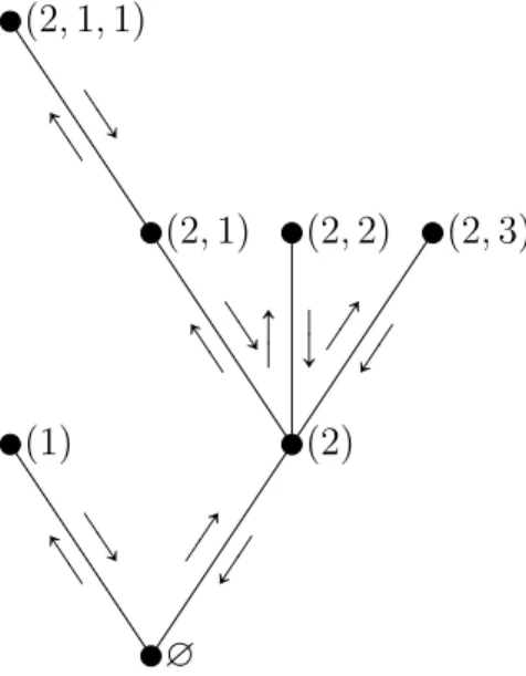
Let us explain briefly how to get the contour function of tree τ . Suppose that τ is the tree shown in Figure 3.2. If we suppose that each edge of τ is drawn such that all of them have unit length, then contour function of τ is the distance (in tree) of a parcel which starts to move from the root and traverse the tree like as shown in Figure 4.1. ∅ Ý Ñ Ð Ý p1q ÝÑ ÐÝ p2q Ý Ñ Ð Ý p2, 1q ÝÑ Ð Ý p2, 1, 1q Ý Ñ Ð Ý p2, 2q ÝÑ ÐÝ p2, 3q
Figure 4.1: Traversing a plane tree and its nodes’ sequences.
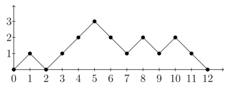
In this traverse, we visit the children from left to right and create their se-quences upon that ordering. Also each edge is traversed two times, so in general, contour function Cs of tree τ is the function
Cs: s P r0, 2|τ |s Ñ r0, |τ |s.
By convention Cs “ 0 for s ą 2|τ |. Note that Cs above might not be surjective1.
In this way it is easy to see that the contour function will look alike the equivalent simple walk of the tree τ which is shown in Figure 4.2.
Proposition 4.2. The mapping τ ÞÑ pC0, C1, ..., C2nq is a bijection from An onto
the set of all Dyck paths of length 2n.
0 1 2 3 4 5 6 7 8 9 10 11 12 1
2 3
Figure 4.2: Contour function of the plane tree in Figure 4.1.
Proof. Mapping 1 in Section 3.3 which we showed that it is a bijection is indeed the mapping in this Proposition.
4.2.2
Galton-Watson Trees
An offspring distribution tpkukě0is simply a probability measure on N0 “ t0, 1, 2, ...u.
Let us define Galton-Watson process.
Definition 4.3. A Galton-Watson process pZnqně0 is a discrete Markov chain
with values in N0 with transition probabilities
P pZn`1 “ k|Zn“ mq “ p˚mk ,
where p˚m
k denotes the m-th convolution power of offspring distribution tpkukě0.
In other words the conditional distribution of Zn`1 given Zn is the distribution
of the sum of Zn i.i.d. random variables with distribution tpkukě0. Initial value
is Z0 “ 1.
If the expected value of a random variable with law tpkukě0 is equal to 1, we
will have some interesting distributions defined below.
Definition 4.4. Probability measure µ on N0 is called critical or subcritical
offspring distribution if 8 ÿ n“0 nµpnq ď 1.[12] We suppose that µp1q ‰ 1.
Now let pNu, u PU1q be a collection of i.i.d. random variables with distribution
µ defined above and indexed by setU. Denote by θ the random subset of U defined by
θ “ u “ pu1, u2, ..., unq PU : @j P t1, 2, ..., nu, uj ď Npu1,u2,...,uj´1q( . (4.1)
Proposition 4.3. θ is a.s. a tree. Also if
Zn“ #tu P θ : |u| “ nu,
pZnqně0 is a Galton-Watson process with offspring distribution µ and initial value
Z0 “ 0.
Proof. If θ is finite then it is a tree, because for every u P θ, due to the definition of θ, we have all of its left siblings and their parents. Also ∅ P θ. In fact Nu is
the number of children of node u.
If θ is infinite, then there exists u “ pu1, u2, ...q P θ for which |u| “ 8. It means that for each n, Nun ą 0, where un “ pu
1, u2, ..., un
q. The probability of this is at most Π8
n“01 ´ µp0q which converges to 0 if µp0q ą 0 which is clearly the
case because µp1q ‰ 1 and ř8
n“0nµpnq ď 1.
The proof that pZnqně0 is indeed a Galton-Watson process can be done easily
by induction.
The finiteness of θ can also be concluded from the fact that the Galton-Watson process with offspring distribution µ becomes extinct a.s.: Zn “ 0 for n large.
Definition 4.5. The tree θ defined by (4.1), or any random tree with the same distribution is called Galton-Watson tree with offspring distribution µ, or in short µ-Galton-Watson tree[12].
Suppose that τ is a tree and 1 ď j ď n∅pτ q, then we denote by Tjτ the branch
that starts from the j-th child of the root:
Tjτ “ tu PU : ju P τu.
We write Πµfor the distribution of θ on the space A. Πµ can be characterized
(i) Πµpn∅ “ jq “ µpjq for every j P N0;
(ii) for every j ě 1 with µpjq ą 0, the branches T1τ, T2τ, ..., Tjτ are
indepen-dent under the conditional probability Πµpdτ |n∅ “ jq and their conditional
distribution is Πµ.
Property (ii) is called the branching property of the Galton-Watson tree.
Proposition 4.4. For every τ P A,
Πµpτ q “
ź
uPτ
µpnupτ qq.
Proof. It is easily understood that knowing that a randomly generated tree θ with offspring distribution µ is the same as τ is equivalent to knowing that for each u P τ , Nu “ nupτ q1! So Πµpτ q “ P pθ “ τ q “ ź uPτ P pNu “ nupτ qq “ ź uPτ µpnupτ qq.
In particular the case when µ “ µ0 for which µ0 is the (critical) geometric
offspring distribution, µ0pnq “ 2´n´1for every n P N0, is interesting and we check
it more in what follows. In that case, the Proposition above tells us that
Πµ0 “ 2
´2|τ |´1,
because for every τ P A, we have ř
uPτnu “ #pτ q ´ 1 “ |τ |.
It means that Πµ0pτ q depends only on |τ |. So the conditional distribution
when given |τ | “ n will be a uniform distribution on An.
Let us check the contour function when µ “ µ0.
1The first clearly implies the second. Knowing that for each u P τ , N
u“ nupτ q, we conclude
that all the nodes u P τ are also in θ and also no other node can be added to θ because for each leaf in v P τ , surely nvpτ q “ 0.
4.3
The Contour Function in the Geometric Case
In general, the contour function does not have a ”nice” probabilistic structure[12].
But when the distribution is the geometric offspring distribution, µ0, there exists
a bijection between Dyck paths and random walks.
Recall that if pSnqně0 is a simple random walk on Z starting from 0, then it
can be written as
Sn“ X1` X2` ¨ ¨ ¨ ` Xn,
where X1, X2, ... are i.i.d. random variables with probability distribution P pXi “
1q “ P pXi “ ´1q “ 12.
We are interested in nonnegative random walks, so put
T “ mintn ě 0 : Sn“ ´1u, (4.2)
and consider the walk from the start until the pn ´ 1q-th walk:
pS0, S1, ..., ST ´1q.
This path in finite a.s. and we call it an excursion of simple random walk. Note that each excursion of simple random walk of length T ´ 1 is also a contour function of a tree with T ´12 edges.
Before stating the next Proposition let us introduce the upcrossing times of random walk S from 0 to 1:
U1 “ mintn ě 0 : Sn“ 1u and V1 “ mintn ě U1 : Sn “ 0u
and for every j ě 1, by induction,
Uj`1 “ mintn ě Vj : Sn “ 1u and Vj`1 “ mintn ě Uj`1 : Sn “ 0u.
If S is an excursion of simple random walk of length T ´ 1, then if we put
it means that S is consisting of K parts that are each positive random walks and due to Markov property they are independent from each other.
If S is a simple random walk (not necessarily an excursion of it) which starts at 0 then for each j “ 1, 2, ..., the part starting at Vj and ending at Uj`1´ 1 can
be either empty or nonempty. Thus S can be partitioned to some i.i.d. simple random walks which endpoints are 0. Denote these parts by ξi (i “ 1, 2, ...) and
also let T0 “ 0 and Ti be the i-th time when S comes back to 0, for i “ 1, 2, ...
(it means that ξi starts at time Ti´1 and ends at time Ti).
The fact that ξi’s are i.i.d., is the essential of excursion theory[19]. To show
that how it can be used for calculations, let us find the distribution of the number of returns to 0 before the time τ “ inftn : Sn “ ´2u. Obviously,
P pξ1 visits ´ 2q ” P pSn“ ´2 for some k with 0 ă k ă T1q
“ P pS1 “ ´1, S2 “ ´2q
“ 1 4. So
P pnumber of returns to 0 before τ , is at least k “ P pexcursions ξ1, ξ2, ..., ξk do not visit ´ 2q
“ P pξ1 does not visit ´ 2qk
“ˆ 3 4
˙k
Proposition 4.5. Contour function of µ0-Galton-Watson tree θ is an excursion
of simple random walk.
Proof. According to Proposition4.2, plane trees are in one-to-one correspondence with Dyck paths. Also Dyck paths are clearly in one-to-one correspondence with nonnegative random walks. Thus the statement of this Proposition is equivalent to saying that the random plane tree θ coded by an excursion of simple random walk is a µ0-Galton-Watson tree. To prove this, suppose that we coded tree θ by
an excursion of simple random walk, S. Now if we consider N , as defined in (4.3), it is easily understood that n∅pθq “ N and for every i P 1, 2, ..., N , the branch Tiθ
is coded with the path pωipnqq0ďnďVi´Ui´1, where for each n P t0, 1, ..., Vi´ Ui´ 1u
ωipnq “ SUi`n´ 1.
Also N is distributed according to geometric offspring distribution µ0 and
conditioned on N “ m, paths ω1, ω2, ..., ωm are independent excursions of simple
random walks. Now according to characterization of Πµ0 these who that θ is a
µ0-Galton-Watson tree.
4.4
Brownian Excursions
In Section 3.4 we talked briefly about Brownian motions and also normalized Brownian excursions. We defined Brownian motions by limit of simple random walks when rescaled properly. In this section we talk about Brownian excur-sions in more depth and we show that the contour function of a tree uniformly distributed over An converges in distribution as n Ñ 8 towards a normalized
Brownian motion.
4.4.1
Local Time Process and Excursion Space
Consider a standard linear Brownian motion B “ pBtqtě0 starting from 0. We
define local time process of Brownian motion B as follows.
Definition 4.6. The local time process pLx
tqtě0 of standard linear Brownian
mo-tion B at level x is mathematically defined by1
Lxt “ żt
0
δpx ´ Bsqds,
where δ is the Dirac delta function2. It can be approximated a.s. for every t ě 0 by Lxt “ lim εÑ0 1 2ε żt 0 1rx´ε,x`εspBsqds. 1
Some authors denote the Local time process by lpt, xq
2It is zero for all values except at zero and its integral over any interval containing zero is
We are particularly interested in local time process at level 0. Now if we define the reflected Brownian motion by βt “ |Bt|, the local time process at level 0 of
Bt or of βt is approximated a.s. for every t ě 0 by
L0t “ lim εÑ0 1 2ε żt 0 1r´ε,εspBsqds “ lim εÑ0 1 2ε żt 0 1r0,εspβsqds.
Thus local time process is a continuous increasing process. The increasing points of this process at level 0 is the zero set of Bt,
ZB “ tt ě 0 : Bt“ 0u,
which is the same as Zβ. If we define the right-continuous inverse of the local
time process as
σl :“ inftt ě 0 : L0t ą lu
for every l ą 0, we will have
Zβ “ tσl : l ě 0u Y tσl´ : l P Du
where D denotes the countable set of all discontinuity times of mapping l Ñ σl.
excursion intervals (away from 0) of β are any connected component of the open set R`zZβ. Then excursion intervals away from 0 of β are intervals of the
form pσl´, σlq where l P D. We define the excursion el “ pelptqqtě0 associated to
the interval pσl´, σlq for every l P D by
elptq “
#
βσl´`t if 0 ď t ď σl´ σl´,
0 if t ą σl´ σl´.
In fact different excursions el are defined somewhat like ωi’s in Proposition 4.5.
We view these excursions as elements of the excursions space E that is defined as follows[12].
Definition 4.7. The excursion space E is a metric space with elements
and metric d,
dpe, e1
q “ sup
tě0
|eptq ´ e1ptq| ` |ζpeq ´ ζpe1q|,
and with the associated Borel σ-field. ζpeq above is defined by
ζpeq :“ supts ą 0 : epsq ą 0u
where sup ∅ “ 0.
Note that zero function does not belong to the excursion space because we require ζpeq ą 0 and ζpeq can be seen as the length of excursion e. Also for every l P D, ζpelq “ σl´ σl´.
4.4.2
The Itˆ
o Excursion Measure
Put qtpxq “ x ? 2πt3 exp ˆ ´x 2 2t ˙ . (4.4)
The function t Ñ qtpxq is the density of first hitting time of x by B[12] (starting
at 0) or of first hitting time of 0 by a linear Brownian motion which starts at x[11].
Itˆo measure npdeq of positive excursions is an infinite measure on the set of elements of excursion space E and has the following two (characteristic) proper-ties[11]:
(i) For every t ą 0 and every measurable function f : R` Ñ R` such that
f p0q “ 0, ż npdeqf peptqq “ ż8 0 dxqtpxqf pxq;
(ii) if t ą 0 and Φ and Ψ are two nonnegative measurable functions defined respectively on Cpr0, ts, R`q and CpR`, R`q, then
ż
npdeqΦpeprq, 0 ď r ď tqΨpept ` rq, r ě 0q
“ ż
where Exis the set of excursions e for which epsq ą x if and only if s P p0, σq
for some positive σpeq1, pBtqtě0 is a linear Brownian motion which starts at
x and T0 “ infZB
The following theorem is the basic result of excursion theory in our particular setting.
Theorem 4.1 (Itˆo). The point measure
ÿ
lPD
δpl,elqpdsdeq
is a Poisson measure on R`ˆ E, with intensity
ds b npdeq
where npdeq is a σ-finite measure on E.
A proof of this Theorem can be found in an article by L. C. G. Rogers[19]. The measure npdeq is called the Itˆo excursion measure. From standard prop-erties of Poisson measures we can conclude the next Corollary.
Corollary 4.1. Suppose A be a measurable set of E with finite positive measure. Put TA“ inftl P D : elP Au. Then TA is exponentially distributed with parameter
of the measure of A, npAq, and the distribution of eTA is the conditional measure
np.|Aq “ np¨ X Aq npAq .
Moreover, TA and eTA are independent.
This corollary can be used for calculating various distributions like height and length of excursions, under the Itˆo excursion measure.
The distribution of height of excursion eptq is
n ˆ sup tě0 eptq ą ε ˙ “ 1 2ε
and its length distribution is
n pζpeq ą εq “ ?1 2πε.
The Itˆo excursion measure have scaling property: For every λ ą 0, define mapping Φλ : E Ñ E by putting Φλpeqptq “
?
λept{λq, for every e P E and t ě 0. Then we have Φλpnq “
? λn.
The scaling property is especially useful when defining conditional versions of Itˆo excursion measure[12]. Let us discuss npdeq when conditioning with respect
to length ζpeq.
There exists a unique collection of probability measures pnpsq, s ą 0q on E
with the following properties[12]:
(i) for every s ą 0, npsqpζ “ sq “ 1;
(ii) for every λ ą 0 and s ą 0, we have Φλpnpsqq “ npλsq;
(iii) for every measurable subset A of E,
npAq “ ż8 0 npsqpAq ds 2?2πs3. Notice that ds
2?2πs3 can be seen as the measure of the set of excursions like e
with length ζpeq P ds. We may and will write npsq “ np¨|ζ “ sq, and the measure
np1q is called the law of the normalized Brownian excursions.
Before continuing, let us first state the famous Radon-Nikodym theorem.
Theorem 4.2 (Radon-Nikodym). If µ and λ are two σ-finite measures on mea-surable space pX, Σq and µ is absolutely continuous1 with respect to λ, then there
is a measurable function f on X taking values in r0, 8q such that for any mea-surable set A
µpAq “ ż
A
f dλ.
The following Proposition emphasizes the Markovian properties of n[12].
1Measure µ is absolutely continuous with respect to measure λ if µpAq “ 0 for every set A
Proposition 4.6. The Itˆo excursion measure n is the only σ-finite measure on excursion space E that specifies the following two properties:
(i) for every t ą 0, and every f P CpR`, R`q,
n`fpeptqq1tζątu ˘ “ ż8 0 f pxqqtpxqdx;
(ii) let t ą 0. Under the conditional probability measure np¨|ζ ą tq, the pro-cess pept ` rqqrě0 is Markov with the transition kernels of Brownian motion
stopped upon hitting 0.
We can use this Proposition to establish the absolute continuity properties of the conditional measures npsq with respect to n. By Radon-Nikodym theorem
this is equivalent to saying that for any measurable set A in excursion space and some measurable function f
npsqpAq “
ż
A
f dn.
Here f is called the Radon-Nikodym derivative of npsq. Now let us denote the
σ-field on E generated by the mappings r Ñ eprq, for every t ě 0 and 0 ď r ď t, by Ft. If 0 ă t ă 1, then the measure np1q is absolutely continuous with respect
to n on the σ-field Ft and the Radon-Nikodym derivative, f , will be equal to
dnp1q dn ˇ ˇ ˇ ˇ Ft peq “ 2 ? 2πq1´tpeptqq.
Using the derivative above we can derive the density of the distribution of pept1q, ept2q, ..., eptpq under np1qpdeq for every integer p ě 1 and every choice of
0 ă t1 ă t2 ă ¨ ¨ ¨ ă tp ă 1[12]: 2?2πqt1px1qp ˚ t2´t1px1, x2qp ˚ t3´t2px2, x3q ¨ ¨ ¨ p ˚ tp´tp´1pxp´1, xpqq1´tppxpq, (4.5) where p˚ tpx, yq “ ptpx, yq ´ ptpx, ´yq, t ą 0, x, y ą 0,
shows that law of peptqq0ďtď1 under np1q is invariant under time reversal.
4.5
Convergence of Contour Functions Towards
Brownian Excursions
The convergence of contour functions to Brownian excursions can be seen as a special case of results provided in article The continuum random tree III by Aldous[1]. Before proving this convergence let us first present two lemmas.
Lemma 4.1. For every ε ą 0,
lim nÑ8supxPRsupsěε ˇ ˇ ? nP`Stnsu “Xx ? n\ or Xx?n\` 1˘´ psp0, xq ˇ ˇ“ 0.
This lemma is a very special case of classical local limit theorems and can be easily obtained by direct calculations, using the explicit form of the law of Sn and
Stirling’s formula[12].
On the other hand the next lemma is a special case of famous Kemperman’s formula[18].
For every integer ` P Z, denote a probability measure under which the simple random walk S starts from ` by P`.
Lemma 4.2. For every ` P N0 and every integer n ě 1,
P`pT “ nq “
` ` 1
n P`pSn “ ´1q.
Proof. There are several different proofs to this lemma[12;18], but we will provide a more enumerative combinatorial proof.
If both sides of the equation above are 0, then there is nothing to prove. Otherwise let us propose a simple question and solve it first.
Question 4.1. Suppose that we have k ”X” and k ` l ”Y”. In how many ways we can put them in a line that for no initial segment the number of Y’s be more than l more than X’s.
For solving this question we can make a bijection to count the number of wrong sequences as we did for Dyck words, and then subtract it from the number of all sequences. Suppose that we have a wrong sequence of X’s and Y ’s. Consider the shortest initial segment in which we have exactly k1 X and pk1
` l ` 1q Y . Interchange all the other X’s and Y ’s that come after this segment. Now we will have a sequence of pk ´ 1q X and pk ` l ` 1q Y . It is easy to see that this is a bijection. So the solution will be equal to
ˆ2k ` l k ˙ ´ˆ2k ` l k ´ 1 ˙ “ p2k ` lq! k!pk ` lq! ´ p2k ` 1q! pk ´ 1q!pk ` l ` 1q! “ pk ` l ` 1qp2k ` lq! ´ kp2k ` lq! k!pk ` l ` 1q! “ pl ` 1qp2k ` lq! k!pk ` l ` 1q! “ l ` 1 k ` l ` 1 ˆ2k ` l k ` l ˙ .
Note that if we put l “ 0 in question above, we get the k-th Catalan number as the solution and if we put n´`´12 instead of k and ` instead of l in above question1,
we will get 2 ` ` 1 n ` ` ` 1 ˆ n ´ 1 n``´1 2 ˙ ,
which is equivalent to the number of random walks like S that start from `, for which we have Sn´1 “ 0 and for no i “ 0, 1, ..., n ´ 1, Si “ ´1. So it is equal to
the number of random walks starting from ` and for which T “ n. Coming back to proof of the lemma, note that it is enough to prove
P`pT “ n | Sn “ ´1q “
l ` 1 n .
It is equal to the number of random walks reaching -1 from ` for the first time in n-th step divided by number of all random walks starting from ` and reaching to
1Note that n´`´1
2 and thus
n``´1
2 are integers if and only if the probabilities defined in the
0 or -2 at pn ´ 1q-th step. So P`pT “ n | Sn“ ´1q “ 2n```1``1 `n``´1n´1 2 ˘ ` n´1 n``´1 2 ˘ ``n```1n´1 2 ˘ “ 2 ``1 n```1 1 ` n´`´1n```1 “ 2n```1``1 2n n```1 “ l ` 1 n .
Using two lemmas above we can prove the following theorem which says that contour functions of random trees in An converge to Brownian excursions as
n Ñ 8.
Theorem 4.3. For every n P N, let θn be a random tree uniformly distributed
over An, and let pCnptqqtě0 be its contour function. Then
ˆ 1 ? 2nCnp2ntq ˙ 0ďtď1 pdq ÝÝÝÑ nÑ8 petq0ďtď1
where e is a normalized Brownian excursion distributed according to np1q and the
space Cpr0, 1s, R`q is equipped with the topology of uniform convergence.
Proof. Using Proposition4.5 and that Πµ0p¨ | |τ | “ nq coincides with the uniform
distribution over An, we get that pCnp0q, Cnp1q, ..., Cnp2nqq is distributed as an
excursion of simple random walk conditioned to have length 2n. Thus we need to verify that the law of
ˆ 1 ? 2nSt2ntu ˙ 0ďtď1
given that T “ 2n ` 1 converges to np1q as n Ñ 8. This can be seen as a
conditional version of Donsker’s theorem. We will divide the proof into two parts: Proving the convergence of finite-dimensional marginals and then establishing the tightness of the sequence of laws[12].
Finite-dimensional marginals. Let us first consider one-dimensional marginals and then base the proof of higher dimensional marginals on it. Fix t P p0, 1q and we will show that
lim nÑ0 ? 2nP ´ St2ntu “ Y x?2n ] or Y x?2n ] ` 1 | T “ 2n ` 1 ¯ “ 2 ? 2πqtpxqq1´tpxq, (4.6) uniformly when x varies over a compact subset of p0, 8q. Note that right hand side of the above equation is the same as (4.5) for p “ 1. It means that the law of St2ntu
?
2n under P p¨ | T “ 2n ` 1q converges to the law of eptq under np1qpdeq.
For every i P t1, 2, ..., 2nu and ` P N0,
P pSi “ ` | T “ 2n ` 1q “ P ptSi “ `u X tT “ 2n ` 1uq P pT “ 2n ` 1q . But P ptSi “ `u X tT “ 2n ` 1uq “ P ptSi “ `, T ą iu X tT “ 2n ` 1uq “ P ptSi “ `, T ą iuqP`pT “ 2n ` 1 ´ iq, also
P`pT “ i ` 1q “ P`ptSi`1“ ´1u X tSi “ 0, T ą iuq
“ P`pSi`1 “ ´1 | Si “ 0qP`pSi “ 0, T ą iq
“ 1
2P`pSi “ 0, T ą iq, both because of markovian property of S. Also
P`pSi “ 0, T ą iq “ P pSi “ `, T ą iq
Thus P pSi “ ` | T “ 2n ` 1q “ 2P`pT “ i ` 1qP`pT “ 2n ` 1 ´ iq P pT “ 2n ` 1q “ 2p2n ` 1qpn ` 1q 2 pi ` 1qp2n ` 1 ´ iq ¨ 2P`pSi`1 “ ´1qP`pS2n`1´i “ ´1q P pS2n`1 “ ´1q , (4.7)
where we used Lemma 4.2 for deriving the second equality1.
Recall that ptp0, xq “ pt{xqqtpxq where qtpxq is defined as (4.4), so
ptp0, xq “ t x ¨ x ? 2πt3 exp ˆ ´x 2 2t ˙ “ ?1 2πtexp ˆ ´x 2 2t ˙ . (4.8)
As an important special case, when x :“ 0, we get ptp0, 0q “ p2πtq´
1 2. For large n, P pS2n`1 “ ´1q « P pS2n “ 0q « p1?p0, 0q 2n “ ?1 2n ¨ 1 ? 2π,
using Lemma4.1if we set x :“ 0, s :“ 1 and n :“ 2n in the second approximation. Also we have the approximations
2n ` 1 t2ntu ` 1 « 1 t and pXx?2n\` 1q2 2n ` 1 ´ t2ntu « x2¨ 2n 2n ´ 2nt « x2 1 ´ t.
Using all of the approximations above we get 2p2n ` 1qpXx?2n\` 1q2 pt2ntu ` 1qp2n ` 1 ´ t2ntuq ¨ 1 P pS2n`1 “ ´1q « 2?2π?2n x 2 tp1 ´ tq. (4.9) 1Note that P `“ P when ` “ 0.
Again using Lemma 4.1, we have the approximation Ptx? 2nuortx?2nu`1pSt2ntu`1 “ ´1qPtx?2nuortx?2nu`1pS2n`1´t2ntu“ ´1q « ptp0, xqp1´tp0, xq 2n “ tp1 ´ tq x2¨ 2n qtpxqq1´tpxq, (4.10)
where in general with P` or `1we mean P``P`1. Now by multiplying approxiamtions
(4.9) and (4.10) to each other and putting i “ t2ntu and ` “ Xx?2n\ or ` “ Xx?2n\` 1 in right hand side of (4.7) we get
P pSt2ntu “ Y x?2n ] or Y x?2n ] ` 1 | T “ 2n ` 1q « 2 ? 2π ? 2n qtpxqq1´tpxq, and the proof of (4.6) is complete.
For higher dimensional marginals we can use a similar way. For example for two-dimensional marginals, we can observe that if 0 ă i ă j ă 2n and if ` P N0,
P pSi “ `, Sj “ m, T “ 2n ` 1q
“ 2P`pT “ i ` 1qP`pSj´i “ m, T ą j ´ iqPmpT “ k ` 1 ´ jq.
Here, only the middle term, P`pSj´i “ m, T ą j ´ iq, needs a treatment that we
didn’t discuss before. However we can see that
P`pSj´i “ m, T ą j ´ iq “ P`pSj´i “ mq ´ P`pSj´i “ ´mq, (4.11)
because if for a random walk that passed through ´1 and yet arrived to m at pj ´ iq-th step, we reflect the part from the first time that random walk hit ´1 to the end, we get a random walk that arrives to ´m at pj ´ iq-th step. It is easy to see that it is also a bijection. On the other hand, by putting i “ t2nsu, j “ t2ntu and ` “ tx?2nu or ` “ tx?2nu ` 1 in (4.11) and then using Lemma4.1, we get
Ptx? 2nuortx?2nu`1 ´ St2ntu´t2nsu“ ty ? 2nu ¯ « pt´sp0, y ´ xq? 2n “ pt´s?px, yq 2n .
Similarly Ptx? 2nuortx?2nu`1 ´ St2ntu´t2nsu “ t´y ? 2nu ¯ « pt´sp0, ´y ´ xq? 2n “ pt´s?px, ´yq 2n . Subtracting the second approximation from the first, we get
P tx?2nuortx?2nu`1 ´! St2ntu´t2nsu “ ty ? 2nu ) X tT ą t2ntu ´ t2nsuu ¯ « p ˚ t´spx, yq ? 2n ,
and the result follows in a straightforward way (approximating the other two terms as previous way and putting this approximation for the middle term, we get want we want).
Tightness. Let px0, x1, ..., x2nq be a Dyck path with length 2n, and for each
i P t0, 1, ..., 2n ´ 1u and j P t0, 1, ..., 2ku, set
xpiqj “ xi` xi‘j ´ 2 min
i^pi‘jqďmďi_pi‘jqxm
with the notation i ‘ j “ i ` j if i ` j ď 2n and i ‘ j “ i ` j ´ 2n if i ` j ą 2n. Proposition 4.7. For each i P t0, 1, ..., 2n ´ 1u, pxpiq0 , x
piq 1 , ..., x
piq
2nq is also a Dyck
path, where xpiqj is defined as above.
Proof. We should prove that xpiq0 “ 0, xpiq2n “ 0 and for each k P t1, ..., 2nu, ˇ ˇ ˇx piq k ´ x piq k´1 ˇ ˇ ˇ “ 1. By definition we have
xpiq0 “ xi` xi‘0´ 2 min
i^pi‘0qďmďi_pi‘0qxm
“ xi` xi´ 2 min i^iďmďi_ixm
“ 2xi` ´2xi