Anchor centric virtual coordinate systems in wireless sensor networks: from self-organization to network awareness

(1)

DISSERTATION

ANCHOR CENTRIC VIRTUAL COORDINATE SYSTEMS IN WIRELESS SENSOR NETWORKS: FROM SELF-ORGANIZATION TO NETWORK AWARENESS

Submitted by Dulanjalie C. Dhanapala

Department of Electrical and Computer Engineering

In partial fulfillment of the requirements For the Degree of Doctor of Philosophy

Colorado State University Fort Collins, Colorado

Fall 2012

Doctoral Committee:

Advisor: Anura P. Jayasumana Michael Kirby

Ali Pezeshki Indrakshi Ray

(2)

ii ABSTRACT

ANCHOR CENTRIC VIRTUAL COORDINATE SYSTEMS IN WIRELESS SENSOR NETWORKS: FROM SELF-ORGANIZATION TO NETWORK AWARENESS

Future Wireless Sensor Networks (WSNs) will be collections of thousands to millions of sensor nodes, automated to self-organize, adapt, and collaborate to facilitate distributed monitoring and actuation. They may even be deployed over harsh geographical terrains and 3D structures. Low-cost sensor nodes that facilitate such massive scale networks have stringent resource constraints (e.g., in memory and energy) and limited capabilities (e.g., in communication range and computational power). Economic constraints exclude the use of expensive hardware such as Global Positioning Systems (GPSs) for network organization and structuring in many WSN applications. Alternatives that depend on signal strength measurements are highly sensitive to noise and fading, and thus often are not pragmatic for network organization. Robust, scalable, and efficient algorithms for network organization and reliable information exchange that overcome the above limitations without degrading the network’s lifespan are vital for facilitating future large-scale WSN networks.

This research develops fundamental algorithms and techniques targeting self-organization, data dissemination, and discovery of physical properties such as boundaries of large-scale WSNs without the need for costly physical position information. Our approach is based on Anchor Centric Virtual Coordinate Systems, commonly called Virtual Coordinate Systems (VCSs), in which each node is characterized by a coordinate vector of shortest path hop distances to a set of anchor nodes. We develop and evaluate algorithms and techniques for the following tasks associated with use of VCSs in WSNs: (a) novelty analysis of each anchor coordinate and compressed representation of VCSs; (b) regaining lost directionality and identifying a ‘good’ set of anchors; (c) generating topology preserving maps (TPMs); (d) efficient and reliable data dissemination, and boundary identification without physical information; and (f) achieving network awareness at individual nodes.

(3)

iii

After investigating properties and issues related to VCS, a Directional VCS (DVCS) is proposed based on a novel transformation that restores the lost directionality information in VCS. Extreme Node Search (ENS), a novel and efficient anchor placement scheme, starts with two randomly placed anchors and then uses this directional transformation to identify the number and placement of anchors in a completely distributed manner. Furthermore, a novelty-filtering-based approach for identifying a set of ‘good’ anchors that reduces the overhead and power consumption in routing is discussed. Physical layout information such as physical voids and even relative physical positions of sensor nodes with respect to X-Y directions are absent in a VCS description. Obtaining such information independent of physical information or signal strength measurements has not been possible until now. Two novel techniques to extract Topology Preserving Maps (TPMs) from VCS, based on Singular Value Decomposition (SVD) and DVCS are presented. A TPM is a distorted version of the layout of the network, but one that preserves the neighborhood information of the network. The generalized SVD-based TPM scheme for 3D networks provides TPMs even in situations where obtaining accurate physical information is not possible. The ability to restore directionality and topology-based Cartesian coordinates makes VCS competitive and, in many cases, a better alternative to geographic coordinates. This is demonstrated using two novel routing schemes in VC domain that outperform the well-known physical information-based routing schemes. The first scheme, DVC Routing (DVCR) uses the directionality recovered by DVCS. Geo-Logical Routing (GLR) is a technique that combines the advantages of geographic and logical routing to achieve higher routability at a lower cost by alternating between topology and virtual coordinate spaces to overcome local minima in the two domains. GLR uses topology domain coordinates derived solely from VCS as a better alternative for physical location information. A boundary detection scheme that is capable of identifying physical boundaries even for 3D surfaces is also proposed.

“Network awareness” is a node’s cognition of its neighborhood, its position in the network, and the network-wide status of the sensed phenomena. A novel technique is presented whereby a node achieves network awareness by passive listening to routine messages associated with applications in

(4)

iv

large-scale WSNs. With the knowledge of the network topology and phenomena distribution, every node is capable of making solo decisions that are more sensible and intelligent, thereby improving overall network performance, efficiency, and lifespan.

In essence, this research has laid a firm foundation for use of Anchor Centric Virtual Coordinate Systems in WSN applications, without the need for physical coordinates. Topology coordinates, derived from virtual coordinates, provide a novel, economical, and in many cases, a better alternative to physical coordinates. A novel concept of network awareness at nodes is demonstrated.

(5)

v

ACKNOWLEDGEMENTS

First and foremost I offer my sincere gratitude to my advisor, Prof. Anura P. Jayasumana, for his guidance, support and encouragement in every single step of my graduate life. Special thanks to Prof Michael Kirby, Prof Ali Pezeshki and Prof Indrakshi Ray for being in my PhD committee and for their valuable guidance.

I would also like to acknowledge my husband, Thilan Ganegedara and my parents for their constant support, guidance, encouragement and scarifies to make my dream come true. Special thanks to my colleagues, Zheng Wang, Vidarshana Bandara, Saket Doshi and Dilum Bandara for their support in many respects during my PhD study.

(6)

vi

TABLE OF CONTENTS

NETWORK-AWARENESS IN WIRELESS SENOR NETWORKS - FOR INTELLIGENT ORGANIZATION AND EFFICIENT DATA DISSEMINATION

1 Introduction……….. 1

2 Problem Statement……… 8

2.1 Challenges in sensor networks………. 8

2.2 Efficient and reliable network organization and data dissemination……… 11

2.3 Research goal and objectives……… 13

3 Dimension Reduction of Virtual Coordinate Systems in Wireless Sensor Networks…….. 20

3.1 Introduction……….. 20

3.2 Novelty of a new anchor……….. 23

3.3 Reducing dimensionality of VCS………. 24

3.4 Dimension size selecting criteria……….. ₂₆

3.5 Reducing dimensionality based on anchors’ VC……….. 27

3.6 Implementation in sensor networks………. 28

3.7 Performance analysis……… 29

3.8 Conclusions……….. 36

4 Directional Virtual Coordinate Systems for Wireless Sensor Networks……….. 38

4.2 Directionless virtual space to directional virtual space transformation……… 41

4.3 Routing in directional virtual domain……….. 45

4.4 Simulation results: partitions in directional virtual space……… 50

4.5 Directional Virtual Coordinate Routing - DVCR……… 50

4.6 Performance of Directional Virtual Coordinate Routing………. 52

5 Topology Preserving Maps from Virtual Coordinates for Wireless Sensor Networks…… 57

5.1 Introduction………. 57

5.2 Background……….. 60

5.3 Topology preserving maps for 2-d and 3-d WSNs……….. 65

5.4 A metric for evaluating 2-d topology preservation ………. 77

5.5 Results……….. 80

5.6 Realizations, applications and extensions……… 86

5.7 Discussion……… 89

5.8 Conclusions ………. 93

6 PMDS: Partial Multi-Dimensional Scaling for Sensor Networks……… 95

(7)

vii

6.2 Methodology……… 96

6.3 Realization of the topology map generation………. 99

6.4 Results……….. 101

6.5 Conclusion……… 104

7 Anchor Placement and TPMs in WSNs – A Directional Ordinate Based Approach……... 105

7.1 Introduction………. 105

7.2 Anchor selection and routing in virtual coordinate systems……… 109

7.3 Properties of directional VC space……….. 111

7.4 Extreme Node Search (ENS) - an anchor selection algorithm………. 115

7.5 Effectiveness of ENS anchors……….. 118

7.6 Related work-topology preserving maps……….. 123

7.7 Topology preserving maps from directional virtual coordinates……….. 124

8 Geo-Logical Routing: Unified Virtual and Topological Space Routing……….. 132

8.2 Related work………. 136

8.3 Topological coordinates from virtual coordinate system………. 141

8.4 Generalized physical and virtual space routing: Geo-Logical Routing……… 148

8.5 Performance of GLR……… 153

9 On Topology Mapping and Boundary Detection of Sensor and Nano networks Deployed on 2-D and 3-D Surfaces……… 169

9.2 Related works………... 171

9.3 Topology preserving maps of 3D surfaces………... 176

9.4 Results – 3D topology preserving maps……….. 181

9.5 Sensor network boundaries……….. 182

9.6 Simulation results: network and event boundary detection……….. 188

10 Network Awareness via Self Learning at Wireless Sensor Nodes……….. 193

10.2 Related work and background……….. 197

10.3 Network-awareness from randomly routed network traffic……….. 201

10.4 Performance analysis of self-learning scheme……….. 211

10.5 Topology awareness – applications……….. 226

11 Recovery Bounds and Phenomena Awareness in WSNs - a Compressive Sensing Based Approach……….. 233

(8)

viii

11.2 Related work……… 236

11.3 Recovery bounds for sparse function recovery with non-orthogonalization measure………. 239

11.4 Compressive sensing under random walk based sampling in discrete cosine domain……….. 244

11.5 Performance evaluation of phenomena discovery from random walk based samples………. 249

12 Summary and Future Work……….……… 256

12.1 Research contributions……….……….……….….. 254

12.2 Future work……….……….……….……… 259

References ……….……….……….……….………. 265

Appendix A CSU benchmark nets and their virtual coordinate generation……….…. 276

Appendix B Simulator for topology map generation, directional virtual coordinate generation and routing algorithms……….……….………….. 284

(9)

ix

LIST OF TABLES

Table 3.1 - Maximum, minimum and average novelty based coordinate set size with 40

initial anchors, in 15 configurations of networks in figure 3.1. A), b)and c)… 36

Table 4.1 - Notations used in the text and theorems in Chapter 4……….……….. 42

Table 4.2 - Example VC transformation steps in 1D network shown in figure 4.1………. 43

Table 5.1 - Notations used in Chapter 5……….……….………. 66

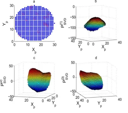
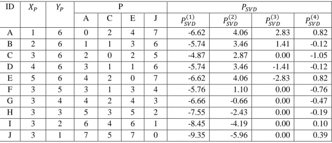
Table 5.2 - Physical coordinates, virtual coordinates and topological coordinates for the network in figure 5.4(a)……….……….……….. 72

Table 5.3 - Computational complexity and memory usage comparison……….…. 73

Table 5.4 - Four different topology map generation approaches for WSNs of n nodes and m anchors……….……….……….……… 82

Table 5.5 - Etp for topology maps in figure5.8-10……….……….…… 82

Table 5.6 - Performance comparison of GLR, LCR, CSR and GPSR with 10 anchors….. 87

Table 6.1 - Topology preservation error for figure6.2 and figure6.3……….…… 102

Table 7.1 - Notations used in Chapter 7……….……….……… 110

Table 7.2 - and ofDVCR, CSR, LCR and GPSR……….………… 121

Table 7.3 - Some of the angles between coordinate-pairs in figure 7.9(a) ………. 129

Table 8.2 - Probability of selecting the correct neighbor based on topology coordinates and physical coordinates for the networks in figure8.2……….…….. 145

Table 8.3 - Performance comparison between GLR, LCR, CSR and GPSR with 10 random anchors……….……….……….………... 162

Table 8.4 - Performance of GLR when anchors are strategically placed using ENS…….. 163

Table 8.5 - Active percentile of each mode in routing……….……… 163

Table 8.6 - Performance comparission between 1-GLR-ENS, 0-GLR-ENS, and GPSR under node failures……….……….……….…….. 167

Table 10.1 - Notations used in Chapter 10……….……….………... 202

Table 11.1 - Notation and description used in Chapter 11……….……….... 238

(10)

x

LIST OF FIGURES

Figure 3.1 - Novelty measurement as # anchors increases up to 40 for (a) circular shaped network with three holes in the middle, (b) grid based network with 100 random missing nodes, and (c) odd shaped network ………... 31 Figure 3.2 - Selection of R for network (a) Figure 3.1 (a), (b) Figure 3.1 (b), and (c)

Figure 3.1 (c) ………... 33

Figure 3.3 - GF with entire anchor set (40 anchors) SVD based reduction with dim. 5 (SVD5 w/ entire VC ), anchor coordinate set based SVD reduction with dim. 5(SVD5 w/ Anchors VC ) (a) Figure 3.1 (a), (b)Figure 3.1 (b), and (c)

Figure 3.1 (c) ………... 34

Figure 3.4 - GR with original coordinates (40 anchors), coordinates selected by novelty (Novelty w/ VCS), SVD-based reduction on selected coordinate set by novelty(SVD10), coordinates selected by novelty based on Anchors VC (Novelty w/ Anchors VC), and SVD-based reduction on selected coordinate set by novelty based on anchors VC(SVD10 anchors VC) in network (a) Figure 3.1 (a), (b) Figure 3.1 (b), and (c) Figure 3.1 (c) ………. 35 Figure 4.1 - 1D network with two anchors and ………... 43 Figure 4.2 - (a) Physical map of the grid, and (b) Directional domain map,

Vs. , of 2D grid ………... 44 Figure 4.3 - Constrained tree network with two anchors and ……….. 46 Figure 4.4 - Constrained tree with branches in a branch, which can be modeled as a sub

constrained tree ………... 49

Figure 4.5 - Partitions of (a) spiral shaped network with 421 nodes, (b) a grid based network with 100 randomly missing nodes, (c) a 496-node circular shaped network with three physical voids/holes, (d) a network of 343 nodes mounted on walls of a building, (e) odd shaped network with 550 nodes, based on the sign of the ordinates in transformed domain created by three randomly selected anchors . Transformed domain has three ordinates generated by , , and pairs ………... 51 Figure 4.6 - Pseudo code of DVCR algorithm ………... 53 Figure 4.7 - (a) , (b) , (c) of CSR, LCR, GPSR and DVCR with 5

randomly placed anchors in Spiral, 30 by 30 node Grid with 800 nodes, Circle with 3 holes, building and odd networks ………. 55 Figure 5.1 - (a) Circular network of 707 nodes with 15 anchors, and (b) – (d) First three

PCs , ,and plotted against the phisical positions. Randomly selected anchors are marked in red cirlcles ………... 68 Figure 5.2 - (a) Odd shaped network with 550 nodes with 15 anchors, and (b) – (d)

First three PCs , , and plotted against the phisical positions. Randomly selected anchors are marked in red cirlcles ………... 69 Figure 5.3 - Nature of principal component directions derived from virtual coordinates... 69

(11)

xi

Figure 5.4 - (a) Physical map of a T-shaped example network, and (b) Topology map of the network in (a). ……….……….……….…… 71 Figure 5.5 - (a) A network on a cylindrical surface (900 nodes) Randomly selected 20

anchors are marked in red cirlcles, and (b) topology map of (a) ………. 72 Figure 5.6 _{- First four PCs a)}

, (b) , (c) , and (d) of a cylindrical network plotted as a color map on the surface of the network. ………... 73 Figure 5.7 - (a) A network, (b) a topology map of (a) with a node flip, and (c) a

topology map of (a) with 1800 rotation. ……….……….… 78 Figure 5.8 - (a) Odd shaped network with 550 nodes and 10 random anchors, is

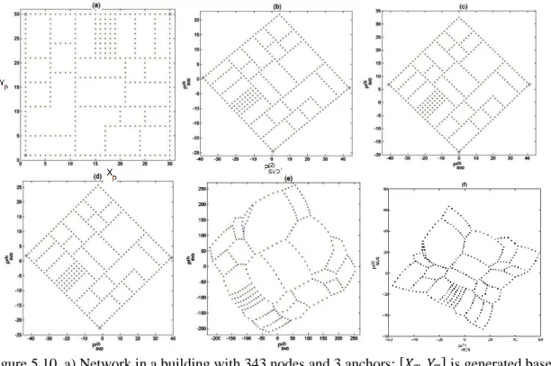
generated based on (b) Case 1: entire VC set, (c) Case 2: anchors’ coordinate set, (d) Case 3: randomly selected nodes’ coordinate set, and (e) Case 4: coordinate set with all the nodes are anchors, (f) MDS………. 81 Figure 5.9 - (a) Circular network with three physical voids with 496 nodes and 10

random anchors, is generated based on, (b) Case 1- entire VC set, (c) Case 2: anchors’ coordinate set (d) Case 3: randomly selected nodes’ coordinate set, and (e) Case 4: coordinate set with all the nodes are anchors

(f) MDS……….……….……….……… 81

Figure 5.10 - (a) Network in a building with 343 nodes and 3 anchors, is generated based on, (b) Case 1- entire VC set, (c) Case 2- anchors’ coordinate set, d) Case 3- randomly selected nodes’ coordinate set, and (e) Case 4- coordinate set with all the nodes are anchors (f) MDS………... 83 Figure 5.11 - 3-D Surface network, consisting of two perpendicular cylinders (T joint)

(1642 nodes, 50 randomly selected anchors): (a) Physical layout, (b) TPM... 87 Figure 5.12 - 3-D Volume network, consisting of a sphere standing on two crossed

cylinders. Sphere has a hole in it. (3827 nodes and 50 randomly selected anchors): (a) physical layout, (b) TPM. ……….……….. 87 Figure 5.13 - VCS corresponding to two anchors in a 1D network……….………. 90 Figure 5.14 - (a) An example network with its ABVCap VCS [113] , (b) TPM only with

ABVCap coordinates in bold black, (c) TPM with all possible ABVCap coordinates of node 12, and (d) TPM from Aligned Virtual Coordinates….. 92 Figure 6.1 - Example network with as an anchor. is a node which is

geodesically apart from . ……….……….…………... 97 Figure 6.2 - (a) 496-node circular network with three physical voids, (b) TPM using

SVD on RSSI based VCS with 15 anchors, (c) TPM using MDS on RSSI based entire VCS with 3 anchors, and (d) TPM using anchors VCs only…... 98 Figure 6.3 - (a) 496-node circular network with three physical voids, (b)TPM using

RSSI based VCS, (c) TPM using MDS, and (d) TPM using anchors VCs

only……….……….……….………... 100

Figure 7.1 - VCs of and its neighbors on a grid with two anchors and ………… 112 Figure 7.2 - and { lines of a circular network with three physical voids where 115

(12)

xii

anchors are at A and B. Only the even numbered lines in the two directions are shown for clarity. ……….……….……… Figure 7.3 - Scatter plot of DVCS coordinate for two sample networks to identify

extreme nodes for anchors. Initial anchor pair is (A1,A2), color corresponds to DVCS value, and highlighted nodes are the identified extreme nodes…. 116 Figure 7.4 - ENS anchor selection algorithm at a node. ……….……… 116 Figure 7.5 - (a) Spiral shaped network with 421 nodes, (b) a 496-node circular shaped

network with three physical voids/holes, (c) a grid based network with 100 randomly missing nodes, (d) a network of 343 nodes mounted on walls of a building, and (e) odd shaped network with 550 nodes. ……….……. 117 Figure 7.6 - Comparison between, greedy ratio of randomly selected anchors from the

boundary/anywhere in the network and that of five anchors selected from ENS for the network in Figure 7.5 (e). ……….……….… 120 Figure 7.7 - DVCS coordinates with respect to anchor pairs: (a) A1, A2, and (b) A3, A4,

for a 9x9 rectangular grid. Arrow indicates the direction of the unit vector... 125 Figure 7.8 - Example to illustrate the angles between different unit vectors ,

, ,and ……….……….………. 126 Figure 7.9 - (a) Odd network. Anchors identified by ENS are indicated in red, (b) TPM

using near orthogonal DVCs, (c) SVD based TPM using the VCS generated using anchors identified by ENS, and (d) SVD based TPM using the VCS generated using 10 randomly placed anchors. ……….………... 128 Figure 7.10 - (a) Circular network with voids. Subset of anchors identified by ENS are

indicated in red, (b) TPM using near orthogonal DVCs, (c) SVD based TPM using the VCS generated using anchors identified by ENS, and (d) SVD based TPM using the VCS generated using 10 randomly placed

anchors. ……….……….……….……… 129

Figure 8.1 - An example physical map to illustrate the effectiveness of combining physical and virtual (connectivity) information for routing. ……….. 133 Figure 8.2 - (a) Spiral shaped network of 421 nodes, (b) Circular network of 496 nodes

with three voids, (c) A 30 by 30 node grid with 100 randomly missing nodes, and (d) Network in a building with 343 nodes. Red circles indicate anchors with ENS anchor placement. ……….……….….. 144 Figure 8.3 - Flow chart of Geo-Logical Routing at a node ……….…………... 146 Figure 8.4 - Pseudo code of GLR algorithms……….……….………… 153 Figure 8.5 - Average Routability of GLR with random and ENS anchor placement

(GLR-R,GLR-ENS respectively), LCR, CSR and GPSR in (a) Spiral network, (b) Circular network with 3 voids, and (c) Sparse grid with 100 missing nodes. GLR-ENS and GPSR are independent from the random

anchor placement..……….……….……….…… 155

Figure 8.6 - Average Path length of GLR with random and ENS anchor placement (GLR-R,GLR-ENS respectively), LCR, CSR and GPSR in (a) Spiral network, (b) Circular network with 3 voids, and (c) Sparse grid with 100 155

(13)

xiii

missing nodes. GLR-ENS and GPSR are independent from the random anchor placement. ……….……….………. Figure 8.7 - Average Energy consumption of GLR with random and ENS anchor

placement (GLR-R,GLR-ENS respectively), LCR, CSR and GPSR in (a) Spiral network, (b) Circular network with 3 voids, and (c) Sparse grid with 100 missing nodes. GLR-ENS and GPSR are independent from the random

anchor placement. ……….……….……….…… 156

Figure 8.8 - Performance of 0-GLR-ENS, 1-GLR-ENS and GPSR original (GPSR-org and GPSR our implementation (GPSR) as the network sparsity vary in a sparse grid. TTL is 100. ……….……….……… 165 Figure 8.9 - Performance of 0-GLR-ENS, 1-GLR-ENS, and GPSR when the TTL vary.

Sparsity of the grid is 16.7%.……….……….……… 166 Figure 9.1 - A network on a cylindrical surface (900 nodes) ……….………. 177 Figure 9.2 _{- Different SVD components for cylinder: (a)}

, (b) , (c) , and (d) ……….……….… ……….……… 180 Figure 9.3 - Topology Generation of a cylinder (900 nodes) ….……… 180 Figure 9.4 - Examples 3D surfaces: (a) Two perpendicular cylinders (T joint), and (b) A

cylinder with a hole (two voids on opposite ends). ….………... 181 Figure 9.5 - Two views of the topology preserving maps for the network on the 3-D

surface of T-joint structure. ….……….….……….….…………... 182 Figure 9.6 - Two views of the topology preserving map of a network deployed on the

cylinder with a hole. ….……….….……….….………. 182 Figure 9.7 - Example network: (a) Sensor network deployed in an area with a lake, (b)

Outer bound of the coverage of the network nodes, and (c) Defined network boundary….……….….……….….……….….……… 183 Figure 9.8 - Relationship between (a) an internal node and its neighbors, and (b) a

boundary node and its neighbors. ….……….….……… 184 Figure 9.9 - Pseudocode of boundary detection algorithm. ….………. 186 Figure 9.10 - Boundary detection results for different network shapes: (a) a spiral

network, (b) a circular network with a C shaped concave void, (c) a circular network with three voids, (d) a square network with an E shaped void, and (e) an odd shaped network. ….……….….……….….……… 189 Figure 9.11 - An example of event boundary detection….……….….……….. 190 Figure 9.12 - Two different views of the 3D boundary identification of two perpendicular

cylinders with no void: (a), (b). ….……….….……… 190 Figure 9.13 - Two different views of the 3D boundary identification of cylinder with

holes: (a), (b). ….……….….……….….………. 190 Figure 10.1 - An example network indicating the virtual coordinate propagation in the

VC developing stage. Network has 7 anchors. ….……….….………… 203 Figure 10.2 - Algorithm for VC estimation at a node. ….……….….……….. 204 Figure 10.3 - Format of a packet in WSN with the added information of VCS. Length of 205

(14)

xiv

the VCS vary….……….….……….….……….. Figure 10.4 - Topological coordinate generation algorithm implemented at each node…... 207 Figure 10.5 - Example networks: (a) Circular network with 496 nodes, (b) Network

deployed on a 3-D surface (T joint) Each cylinder has a radius 2.54 units, height 16 units, and is covered with a grid of 512 nodes, and (c) A network of 343 nodes mounted on walls of a building. Three anchors are manually placed at three corners as shown. Topological coordinate generation algorithm of Figure 10.4. implemented at each node. ….……….. 209 Figure 10.6 - Error in entire VCS of the network ( ) averaged over 10 configurations as

the number of packets traverse in the network increases. Network with 496 nodes and 10 anchors. ….……….….……….….……… 213 Figure 10.7 - Number of packets required for all the nodes to generate error free VCS

averaged over 10 different configurations as TTL varies. Network has 10,20 and 40 anchors respectively for N=496 , 1081 and 2048. ….………... 213 Figure 10.8 - Error in VCS vs. number of packets forwarded by each node without any

VC updates , averaged over 10 anchor placements. ….……….. 214 Figure 10.9 - Percentage of nodes in VC mode vs. the number of packet traversed in the

network averaged over 10 random anchor placements. TTL is 100………… 214 Figure 10.10 - Topology preserving map development at a sample node (identified by

color red). Number of anchors is 10 and total number of nodes is 496. TTL of a packet is 100. ….……….….……….….………. 216 Figure 10.11 - Topology preserving map development at a node of a 3D T-joint assuming

it store the destination topology coordinate of every destination node that goes through it. Number of anchors is 10 and total number of nodes is 512.TTL of a packet is 100. ….……….….……….….………….. 217 Figure 10.12 - Topology preserving map development at a node of a 3D T-joint assuming

it store the destination topology coordinate of every destination node that goes through it. Number of anchors is 10 and total number of nodes is 512.TTL of a packet is 100. ……….……….………. 219 Figure 10.13 - Variation of percentage number of nodes at the observing node Vs. number

of network packets, for circular network with 3 voids (N=h 496, M=10,

H=10). ……….……….……….………. 220

Figure 10.14 - (a-b) Two view of TPMs at two randomly selected nodes after 20000 packets disseminate in the network, (c-d) Common set of nodes that two randomly selected nodes have, (e-f) Set of common boundary nodes at two randomly selected nodes. Nodes on the inner boundary have the same order, which indicates the maps are consistent..……….……… 221 Figure 10.15 - Variation of percentage number of nodes in the topological domain as the

number of packets generated in the network varies. ……….……….. 226 Figure 10.16 - Variation of percentage average routability of the learning network as the

(15)

xv

Figure 11.1 - RW based sample collection on an example grid……….…………... 246 Figure 11.2 - Distributed Phenomena Discovery – Algorithm implemented at a node…… 247 Figure 11.3 - Variation of and number of samples used when (a) s=2 (b) s=3 (c) s=4… 248 Figure 11.4 - (a)Average temperature distribution of State of Alabama in August. 7653

sensors in total are available. (b) Reconstructed image based on 2583 samples collected by a single carrier (c) Reconstructed image at randomly selected node when 1056 samples were collected by that node……….. 251 Figure 11.5 - Variation of average error with number of samples used for reconstruction

in centralized recovery. Single carrier with 4000 steps in total and two carriers with 2000 steps per each were used……….………... 252 Figure 11.6 - Variation of average error with number of samples used for reconstruction

in a distributed manner. Evaluation is after 1000 messages with 300 TTL disseminated in the network.……….……….……… 252 Figure 11.7 - Convergence rate of nodes achieving phenomena awareness in a distributed

(16)

1 CHAPTER 01 INTRODUCTION

The availability of economical, low-power miniature processors and sensors integrated with wireless communication in a single chip has resulted in systems called Wireless Sensor Networks (WSNs). WSNs applications [114] cover a large number of domains spanning physiological, habitat and environmental monitoring, condition-based maintenance, smart spaces [107], military, precision agriculture, transportation, and inventory tracking [56]. WSNs differ considerably from current networked and embedded systems. Although WSNs share the large-scale and distributed nature of other networked systems such as the Internet, their resources and capabilities are extremely limited in comparison. Increasing computing and wireless communication capabilities will expand the role of the sensors from mere information dissemination to more demanding tasks as sensor fusion, classification, and collaborative target tracking. Moreover, since WSNs do not rely on any hard-wired communication links, nodes can be deployed in places without any pre-deployed communication infrastructure.

Future WSNs can be envisioned consisting of hundreds to millions of nodes deployed in inaccessible terrains or structures, monitoring and interacting with environment for long periods of time. Due to the enormous size of such networks, use of costly and highly capable sensor nodes becomes infeasible. The main challenge with such large-scale WSNs is extending the lifespan of the entire sensor network while constructing intelligent

(17)

data-2

accumulating systems. In the process of designing such systems, the following restrictions and constraints have to be considered: (a) limited energy, memory, computational capabilities, and communication bandwidth; (b) cost and complexity of any hardware integrated to each node such as GPS; and (c) susceptibility of measurements such as signal strength to conditions such as fading and noise and the corresponding errors. Advances in technology have produced a vast spectrum of sensor nodes with diverse capabilities. Examples spanning from low-end motes as Radio-Frequency Identification (RFIDs) units priced from $1 to $25, with very little memory (16 bits) [97], to high-end powerful motes such as Imote2 [61] with 32MB RAM, 13MHz to 416MHz processor (Marvell PXA271), which uses three AAA batteries, alleviate the challenge on researchers. Having scalable and less complex algorithms that are capable of structuring networks and supporting data dissemination under the hardware constraints opens up the path for a range of new applications in the area of cyber physical systems [80] as well as ubiquitous networks [80]. This research develops energy- and memory-efficient algorithms as well as techniques that do not require costly additional hardware, thereby facilitating such applications with high reliability.

Virtual coordinates provide an economical alternative to geographical coordinates for routing and self-organization of large-scale WSNs. Geographical coordinate-based protocols such as Geographical Routing (GR) require physical location of nodes, which may be obtained by GPS or a localization algorithm [14]. Use of GPS is too costly and/or is infeasible for many applications. Moreover, localization using analog measurements such as signal strength and time delay is difficult and susceptible to noise, fading, and multipath interferences. Need for accurate power control and signal strength measurements increase the

(18)

3

hardware complexity as well as the cost. Even when geographic coordinates are available, routing is carried out using Line-of-Sight distance information derived from geographic coordinates. Hence, concave physical voids and concave boundaries in the network degrade the performance of GR schemes. Traditional Virtual Coordinate Systems (VCS) characterize each node by a coordinate vector consisting of the shortest path hop distances to a subset of nodes, named anchors. These anchors are a set of ordinary sensor nodes with no additional capabilities than the other nodes in the network. Coordinates can be obtained using a controlled/organized flooding mechanism initiated by the anchors. The number of anchors becomes the network’s dimensionality in the virtual coordinate space. Thus, VCS is a higher dimensional abstraction of a partial connectivity map of sensors. Features such as ease of generation and facilitation of connectivity-based routing without the need for geographical information make VCS an attractive scheme for large-scale, resource-starved WSNs. As the network’s connectivity information is embedded in VCs, the physical voids are transparent in virtual space.

There are three major problems associated with VCS. First, the number of anchors required and their placement for a given network play a crucial role in the performance of VC-based routing algorithms. However, identification of the optimal number of anchors and their proper placement remain as major challenges. Under-deployment of anchors causes identical node coordinates, while over-deployment and improper placement worsen the local minima problem [23],[36], resulting in logical voidsError! Reference source not found.. A node unable to identify a neighbor closer to the destination than itself is called the local minima problem. Not having a proper distance estimation is the second issue. The most commonly used distance estimation is norm 2 without any justification. The third deficiency is due to the fact

(19)

4

that VCS lose the directional information related to the node positions. Thus, existing algorithms based on VCS are limited to routing, and it is difficult to use in many applications as target tracking, boundary detection, etc., where such directional information is crucial. In this research, we go beyond the traditional VCS approaches/algorithms and derive coordinate systems with directional properties that provide efficient replacement of physical coordinate systems for various applications.

This research significantly advances the VCS domain to state-of-the-art by developing fundamental results, efficient algorithms, and techniques to achieve reliable WSN organization and data dissemination techniques. The contributions of this research can be categorized into six main sectors: (a) compressed representation of VCS and novelty analysis of each anchor coordinate; (b) regaining lost directionality and identifying a ‘good’ set of anchors; (c) generating TPMs; (d) efficient and reliable data dissemination schemes; (e) boundary identification without physical information; and (f) self-evolving sensor nets, i.e., each node in the network starts learning about the network and becoming network aware.

In traditional VCSs, an average of 6% of the nodes are used as anchors ; thus, when the network size scales the length of the VC, which is also used as node ID, the VC becomes significantly long. We proposed a compression scheme that provides a compressed representation of the VCS without degrading the original performance. Furthermore, a novelty filtering-based technique for evaluating the amount of novel information contained in an ordinate on the coordinate space created by the rest of the anchors is analyzed. This method can be used to identify unnecessary or inefficient anchors as well as good anchor locations, lowering overhead and power consumption in routing.

(20)

5

When a VCS is generated, the directionality information that allows characterizing relative and absolute node positions is lost due to the radial propagation of the ordinates. A Directional Virtual Coordinate System (DVCS) is proposed based on a novel nonlinear transformation that restores the lost directionality information in the VCS. The introduced virtual directionality alleviates the local minima issue present in the original VCS. The ability to specify cardinal directions based on vector-form representation and use of angle estimations among directions are radical changes from the traditional VC system approaches. Performance of VCS-based algorithms is highly dependent on the anchor selection. A novel anchor-placement scheme, based on directional transformation on two randomly selected anchors, called Extreme Node Search (ENS) is proposed. VCSs based on ENS anchors show significant improvement in underlying algorithms’ performance (routing, map generation, etc.) compared to that of VCSs generated using traditional anchor selection approaches.

Physical layout information such as physical voids, boundaries, and even relative physical position of sensor nodes with respect to X-Y directions is absent in a VCS description, and obtaining the physical topology of such networks has not been possible until now. Two novel techniques to generate Topology Preserving Maps (TPMs) from VCS, based on Singular Value Decomposition (SVD) and DVCS, are presented. In addition, the proposed extension of SVD-based TPMs for 3D networks is applicable not only in WSN context but also in emerging nano-network applications[1][6] where obtaining a physical map is impractical.

The impact of proposed TPM generation without localization is immense in developing new algorithms and concepts. A technique that combines the advantages of geographic and logical routing called Geo-Logical Routing (GLR) to achieve higher routability at a lower cost is designed. It uses topology domain coordinates, derived solely from virtual coordinates

(21)

6

(VCs), as a better alternative for physical location information. A novel routing scheme called Directional Virtual Coordinate Routing (DVCR), which illustrates the effectiveness of the DVCS, is proposed. DVCR significantly outperforms existing VCS routing schemes, while achieving performance similar to the geographical routing scheme, but without the need for node location information. A TPM of a network is an identification of the correct embedding out of all the possible embeddings in the higher dimensional virtual domain, which facilitates the identification of network’s internal and external boundaries without the need of physical location information. The proposed boundary detection is capable of identifying physical/event boundaries in 2D and 3D surfaces. Even though we illustrate the capability of the boundary detection using connectivity-based approach, this scheme can be used with physical information as well.

The future of WSNs can be envisioned as networks that evolve over time, becoming smarter while improving the performance by learning and inferring information about the network and sensed phenomena based on information gleaned from ongoing packet transmissions. Finally, a novel concept of nodes achieving such network awareness by resorting to passive listening at individual nodes’ normal messages associated with data dissemination or network management in large-scale WSNs is discussed. With traditional methods, achieving network awareness requires costly localization integrated with global distribution of location information based on network flooding.

Moving beyond the existing sensor network, applications such as cyber physical systems, smart grids, and ubiquitous networks, require adaptive, self-evolving, reliable algorithms. This research lays a solid foundation for such an algorithm development platform.

(22)

7

The flow of the dissertation is as follows: Chapter 02 discusses the problem statement of the research. A dimension reduction technique and novelty filtering based novel information measure for each anchor in VCSs are proposed in Chapter 03. Furthermore, Chapter 04 discusses a transformation to regain the lost directionality in VCS. After investigating the properties of the proposed Directional Virtual Coordinate System (DVCS), a routing scheme that makes use of the directionality information, is discussed. Singular Value Decomposition (SVD) based TPM generation technique for 2D and 3D networks is addressed in Chapter 05, while Chapter 06 discusses energy efficient partial Multi-Dimensional Scaling based approach for TPM generation using RSSI-based VCSs. Anchor selection is one of the main challenges in VCS. Chapter 07 proposes a scheme called Extreme Node Search that provides a ‘good’ set of anchors, improving the performance not only in routing but also in TPM generation. Moreover, Chapter 07 proposes a less computationally complex DVCS-based TPM generation scheme as well. Applications of TPMs such as routing and boundary detection without the need for physical information are discussed in Chapter 08 and 09, respectively. A proposed routing scheme in Chapter 08, Geo Logical Routing, is a family of routing schemes that probabilistically combines the topological and virtual information to overcome the weaknesses in each other’s domain. A self-learning approach where each node learns and becomes aware of its environment without requiring an expensive and dedicated setup phase is discussed in Chapter 10. Finally, mathematical formulation of limitations in compressive sensing based phenomena reconstruction and its distributed implementation are addressed in Chapter 11. Chapter 12 summarizes and concludes the research work.

(23)

8

CHAPTER 02

PROBLEM STATEMENT

Many emerging Wireless Sensor Network (WSN) applications rely on networks of randomly deployed, wirelessly connected smart sensor nodes that are capable of self-organizing and cooperatively monitoring physical and environmental phenomena. The size of a sensor node (mote) can be as small as a millimeter-scale object that consists of a small-scale processor, memory, and radio. These smart networks (e.g., smart RFID networks, smart grids, etc.) and their spectrum of applications can be characterized by the network size and node capabilities such as communication range, memory, energy, and computational power. Thus, protocol design requirements and constraints vary depending on the target application. Subsection 2.1 discusses the variety of sensor nodes available, their limitations, and challenges in algorithm development. Subsection 2.2 addresses the importance of data dissemination and fusion and the existing challenges. Finally, Subsection 2.3 explains the problem statement and the research contributions.

2.1 Limitations and Challenges in Sensor Networks

The number of nodes in a sensor network may vary from hundreds to tens of thousands depending on the application. Future technology evolutions may result in networks with millions of nodes. Hence, algorithms for WSNs should be scalable in terms of performance

(24)

9

and complexity. For instance, routing/structuring algorithm’s communication, computation, and memory complexities should not drastically increase as the number of nodes increases. Also, in routing algorithms, routing performance should not degrade, and address the length of the addressing scheme should not grow significantly as the network’s size increases. Mostly the network size depends on the deployment area, transmission, and sensing coverage of a sensor node, as well as overall budget. Sensor nodes, in general, are considered to have low memory, low energy, and low computational capabilities. However, such characteristics are highly dependent on the application requirements, network size, and the associated budget.

Sensor nodes that are currently available include RFIDs that are priced from $1 to $25, with very little memory (16 bits) [97], and TelosB [111][74] and Mica2 [60][74], which are priced around $99 with 10KB memory, 250 Kbps radio (CC2420), and a 16‐bit processor (MSP430). There are powerful motes such as Imote2 [61] with 32MB RAM and 13MHz to 416MHz processor (Marvell PXA271). These low-end nodes are usually powered using AA or AAA batteries. Hence, the amount of energy available for processing and communication is strictly limited. It can be thought of as a tradeoff between the number of nodes and their capabilities, under the given budget constraints. Advancements in technology have enabled the existence of miniature and economical sensor nodes that are capable of sensing various types of physical and environmental conditions, data processing, and wireless communication. Large networks can be heterogeneous so that they contain a subset of nodes, which have larger memory, higher battery life, as well as higher computational capabilities. In this research, we are focusing on homogeneous, large-scale static sensor networks that

(25)

10

consist of low-capability sensor nodes that operate with AA batteries, such as MICA2 and TelosB.

As mentioned earlier, most of the low-end sensor nodes are battery powered; therefore, in general it is important to limit power consumption of battery-operated devices in order to extend network’s life span. A sensor node consumes power for sensing, communicating, passive listing, and data processing. Of all the processes running on sensor nodes, data/control message transmission requires the most amount of energy. The cost of wirelessly transmitting 1 Kb of data for a distance of 100 meters, in terms of energy, is approximately the same as that for the execution of three million instructions by a processor of 100 million instructions per second per Watt [74]. Evolving power harnessing technologies will allow sensor nodes to renew their energy from solar sources, temperature differences, or vibration, providing more flexibility in energy conservative algorithm design. Under energy harvesting strategies, for a perpetual sensor node operation, it must satisfy [112], , where and are the generated and consumed average powers, respectively. , and are duty cycle, power consumptions when the node is idle and active, respectively. When is large, (i.e., the node is active for a long period) would be high. Hence may not be sufficient for the long-term operation of the sensor node. Even with certain battery-operated devices, one may need to limit the peak power consumption. As stated in [112], a device with a coin-size battery restricted to consume 200 µW of power on the average, has a lifespan of 167 days, which is equivalent to half a year. In such cases, the power is limited, but nodes are able to pursue long-term strategies to enhance its lifetime. The time it takes to harvest energy required to transmit a packet is / , where is the energy per packet and is the power generated by the harvesting scheme. The duration that

(26)

11

a network is not available for sensing would grow at least linearly with the number of nodes, and it is inversely proportional to the harvested power.

Though computer networks and sensor networks have some similarities, algorithms and protocols used in computer networks cannot be directly used in limited memory and low computational power environments. Thus, novel algorithms/protocols focused on WSNs need to be developed. For instance, storing complete routing tables in a sensor node is impractical. Hence, algorithms should be designed in such a way that they address memory and computational limitations while supporting large-scale networks. Most of the large sensor networks are randomly deployed [116]. In order to perform data dissemination in an efficient manner, networks need be organized. This is also important for other applications such as boundary identification, target tracking, malfunction monitoring of equipments, and habitat monitoring. Manual configuration is not practical due to the size and, in some applications, especially those related to military, due to security purposes. Hence, sensor nodes need to organize themselves, and self-organization should be performed in an efficient and distributed manner even in large-scale networks.

2.2 Efficient and Reliable Network Self-Organization and Data Dissemination

The ability to self-organize and route messages among sensor nodes is key to the deployment of future large-scale Wireless Sensor Networks (WSNs). Routing protocols [4] play a crucial role in information fusion and dissemination in WSNs. They can be broadly categorized as content-based routing and address-based routing [23]. The former uses content-based attributes in the packet to define the destination set [18], while the latter uses some sort of position information, physical or virtual, to identify or to reach the nodes.

(27)

12

Physical domain schemes rely on location or physical position information [4] obtained using localization algorithms or GPS. Equipping nodes with GPS is costly and infeasible for many applications. Localization based on parameters such as RSSI is error-prone and difficult for a network of millions or even hundreds of sensors. If location information is available, Geographic Routing (GR) schemes (also called position-based routing or Geometric Routing) [69] can be used. GR possesses the advantage of having directional information, but its performance is highly correlated with localization errors ‎[106]. GR also suffers from dead-end problems, also known as local minima problems, due to physical voids. A local minima problem is simply when a node currently holding the packet is unable to find a closer neighboring node to the destination than itself.

Virtual Coordinate System (VCS) is an alternative addressing scheme that does not require GPS or additional hardware for signal strength measurements. In VCS, each node is characterized by a length vector, where each ordinate corresponds to the shortest path hop distance to a subset of nodes, called anchors. Therefore, the number of anchors becomes the networks’ dimensionality. This hop-based coordinate system is independent of noise and interference. Furthermore, VCS has connectivity information embedded in each ordinate, so VC routing is less susceptible to ‘local minima’ caused by physical voids.

Performance of algorithms based on VCSs is highly sensitive to the number of anchors and their placement. The coordinates of a node may not be unique due to the insufficient number of anchors and/or their improper placement. The existence of nodes with identical coordinates degrades the routability, which is defined as the percentage of packets that successfully reach their intended destination. Although one can argue that proper anchor selection and placement prevent this problem, guaranteeing such a scenario is difficult and

(28)

13

challenging. In virtual domain routing, similar to its counterparts in physical domain, a packet is greedily forwarded to the closest neighbor to the destination. Greedy forwarding decisions are based on information locally available to a node, i.e., coordinates of its neighbors. However, the distance function from the current node to the destination does not monotonically decrease due to the imperfections of virtual space, causing local minima that degrade the routability. These minima are referred to as logical voids and are analogous to physical voids in the physical domain. As identified, improper anchor placement and over/under placement of anchors are the main causes for this local minima problem. While increasing the number of anchors decreases the likelihood of having multiple nodes with identical coordinates, it may increase the local minima encounters during routing. Finding the overall best anchor placement is extremely challenging and, even if found, it is not likely to eliminate the local minima problem except in a limited set of network topology classes as 1D networks and 2D full grids.

2.3 Research Goal and Objectives

The goal of this research is to facilitate the deployment of large-scale sensor networks and applications by developing and evaluating reliable, efficient algorithms and techniques that do not require physical localization of nodes.

Moving beyond the discussed issues, VCSs also suffer from (a) loss of directionality and (b) lack of physical information such as relative position, voids, and boundaries in virtual domain. Thus, it is impossible to develop algorithms such as boundary detection, geographical routing, target tracking, etc., solely based on VCS. In contrast, if such information can be extracted from VCS, sophisticated algorithms that are based on physical

(29)

14

information can be replaced with location-free VCS-based approaches. Moreover, algorithms that combine the advantages of connectivity information from VCS and derived physical and/or directional information will outperform physical-information-based algorithms. With this knowledge and understanding of VCS issues and their causes, we state the objectives of this research and accomplishments under each objective as follows.

1. Efficient, Scalable and WSN-Friendly, Virtual Coordinate System (VCS) Based Approaches for Self-Organization

Virtual coordinate-based algorithms, such as those for routing, are significantly beneficial by having the connectivity information embedded in the VCs. As explained above, if the number of anchors is insufficient or if they are improperly placed, the network will suffer from identical coordinates and local minima problems. Finding the optimal number of anchors and the proper placement of anchors are difficult problems to solve, especially because they are interrelated. Furthermore, some of the anchors may carry redundant information for a given node pair, and others may provide incomplete information resulting in inaccurate distance values degrading routability. Higher numbers of anchors lessen the problem due to identical coordinates, yet it increases the overall energy consumption due to increased VC address, which is used as node ID, and packet length. None of the existing literature, to our knowledge, presents a method to identify the useful information content of each anchor and reduce the dimensionality of the virtual coordinate space, without degrading the performance of the original coordinate system while decreasing the energy consumption. A novel technique based on novelty filtering that quantifies the novel information content of each ordinate in the remaining space, thus identifying ‘good’ anchors for routing, is

(30)

15

proposed in Chapter 03. Moreover, as the network size increases, the number of anchors required also increases. The higher the coordinate length, the higher the energy consumption is. A compressed representation of VCS, which provides more or less the same or sometimes better performance in routing, is proposed in Chapter 03.

2. Regaining Lost Directionality in VCS

Inadequacies associated with VCS are due to the loss of directionality information and lack of information about the physical topology. A novel transformation with which the VCS can regain its lost directionality (notion of left/right or south/east) is proposed in Chapter 04. Thus, nodes acquire some sense of physical location to supplement the connectivity information embedded in the original VCS. No additional transmission cost is involved as each node can evaluate the directional coordinate values with VCs available locally. First, properties of directional domain are derived. The ability to specify cardinal directions and use angles is a radical change from the traditional VCS approaches. Acquiring directionality provides new information hitherto not available in VCS and empowers a new approach for designing a broad spectrum of WSN algorithms. The technique to identify ‘good’ anchors alleviating the issues in VCS, called Extreme Nodes Search (ENS), is one algorithm among the proposed DVCS-based algorithms that are discussed in Chapter 07.

3. Restoring Physical Layout Information That are Absent in VCS

Many of the problems associated with VCS are due to the lack of information about physical network. Physical layout information such as physical voids, relative physical positions of sensor nodes with respect to X-Y directions, and even explicit connectivity

(31)

16

information are absent in a VCS description. These difficulties can be overcome if information on physical topology is available. Combining VC information and position or direction information in one network essentially would combine the advantages of VC routing and geographic routing schemes. However, this has to be achieved without inheriting the disadvantages associated with obtaining location information or localization. Obtaining topological and directional information from VCS, i.e., VCS to Cartesian coordinate transformation, is challenging. Obtaining the physical topology of a network from the set of VCs has not been possible until now. We developed the theoretical basis and techniques to obtain a topology map that preserves the 2D as well as 3D physical topology of a sensor network, including the geographical voids and relative Cartesian directional information (see Chapters 05 and 06).

A vector-based representation is proposed for the DVC domain, which is then used to introduce the concept of angles between virtual directions in the transformed domain. The ability to specify cardinal directions is a radical change from the traditional VC system approaches. A novel TPM generation scheme is developed by selecting two near orthogonal directions in DVCS, as proposed in Chapter 07. This new TPM generation scheme requires significantly less computations than the existing Principle Component Analysis based methods.

4. Reliable Data Dissemination and Boundary Detection with Localization-Free Approaches

Many difficulties associated with VCS-based schemes are attributable to the lack of information about the physical network. Layout information such as physical voids and

(32)

17

relative positions of sensor nodes with respect to X-Y directions is absent. Even though VCS is based on connectivity, explicit information on hop distances between any pairs of nodes is not available and is difficult to estimate. The absence of connectivity information, on the other hand, is the cause for local minima problems in physical domain routing. Combining connectivity information in VCS and position or direction information in a network would essentially combine the advantages of VC routing and geographic routing schemes overcoming the disadvantages in each other’s domains.

A family of routing schemes called Geographic-Logical Routing (GLR), which combines the topological coordinates solely derived from VCS and VC information to achieve significantly high performance in routability, is developed as discussed in Chapter 08. The proposed non-linear directional transformation that unlocks the directional information in VCS is further investigated and is used in routing. The developed routing algorithm (discussed in Chapter 04), called Directional Virtual Coordinate Routing, provides a significant improvement in routing over existing routing approaches for WSNs.

Boundary detection plays a crucial role in information fusion and dissemination in 2D and 3D WSN applications such as target tracking, plume tracking [64], forest fires, animal migration, underwater WSNs, and surveillance applications. Identifying the boundary is also often important for self-organization of networks. Any network has a specific embedding (configuration) and can have three different types of boundaries: (1) network’s outer boundary, (2) inner boundary, and (3) event boundary. Currently available boundary detection schemes that have been targeted exclusively for 2D networks can be broadly categorized into (1) physical information-based and (2) topological /connectivity information-based. The former uses the physical position of nodes to identify the boundary

(33)

18

while the latter uses topological/connectivity information of the network. Physical domain schemes rely on node location or physical position information obtained using localization algorithms or GPS. A connectivity domain description of a network can have more than one valid embedding, even though only one of them corresponds to the physical network. Identifying the correct embedding, which is the physical topology, solely based on the connectivity information is challenging. Due to such difficulties, there is no connectivity-based approach available to identify boundaries of 3D surfaces, to the best of our knowledge. In Chapter 09, we propose a novel-connectivity-based approach for network and dynamic event boundary detection for 2D and 3D networks.

5. Intelligent Sensor Networks by Self-Learning Approaches

We envision future sensor networks as networks that evolve by long-term learning and inference, achieving over time increasing levels of network awareness, thus becoming smarter and better at what they do. We use the term “network/topology awareness” to indicate a node’s cognizance of the topology, shape, and boundary of the network and its position in that network. Upon initial deployment, the nodes would be quite oblivious of their environment, their location in the network, and the nature of the network that they belong to. The only information that the nodes are aware of is the number of neighbors they have and their IDs. Thus, a network has to rely on random routing schemes for data dissemination. In order to improve the reliability of data dissemination, network organization is critical. On the other hand, having an energy-consuming dedicated network organization phase in resource-limited WSNs reduces the network lifespan. However, over time, the nodes listen to the information disseminated in the network and infer additional knowledge and state

(34)

19

information, leading the nodes and therefore the network to achieve network-awareness. In Chapter 10, we discuss our distributive scheme where nodes start learning from the packets that they forward until each node becomes network-aware. Then we investigated compressive-sensing-based approaches for a node to discover sensed phenomena in the network, thus making nodes phenomena-aware as we discuss in Chapter 11.

(35)

20 CHAPTER 03

DIMENSION REDUCTION OF VIRTUAL COORDINATE SYSTEMS IN WIRELESS SENSOR NETWORKS

3.1 Introduction

Routing protocols for Wireless Sensor Networks (WSNs) can be broadly classified into physical coordinate-based and virtual coordinate-based schemes. Physical domain routing relies on the physical (geographic) position information for routing, e.g., as in geometrical routing [4]. Virtual domain (or logical) routing is based on a set of virtual coordinates that capture the position and route information, e.g., hierarchical/clustering schemes [4] and Virtual Coordinate (VC) based routing [22][23][81]-[101]. The focus of this work is to reduce dimensionality of Virtual Coordinate Systems (VCSs) and thus enhance the energy efficiency without degrading the routability.

Virtual Coordinate based Routing (VCR) relies on a set of anchor nodes. The VCs of a node consist of the hop distance from the node to each of a set of M anchors. The cardinality of the coordinate is the number of anchors. The major advantage of VCR over physical domain routing is that connectivity information is embedded in the VCs; therefore, physical voids that degrade physical domain routing no longer exist in the virtual domain. Moreover, high routability can be achieved without requiring physical localization or GPS.

Most of the VCR schemes [22][23][81]-[101] use Greedy Forwarding (GF) combined with a backtracking algorithm. In GF, a packet is simply forwarded to a neighbor that is

(36)

21

closer to the destination than the node holding the packet. VCs of nodes are used for distance evaluation between nodes as well as for node identification (ID).When a closer neighbor cannot be found, i.e., the packet is at a local minima, backtracking is employed to climb out of it. Existing anchor placement strategies [22][23][101] cannot guarantee unique IDs or 100% Greedy Ratio (GR). GR is defined as the percentage of routing requests that can be completed using GF alone.

The use of logical coordinates for routing has its own drawbacks. If the number of anchors is not sufficient or if they are not properly placed, the network will suffer from identical coordinates and local minima problems. As [34] and [36] explain, the anchors may cause local maxima in the distance function at their locations, and hence minima at other node locations. To avoid local minima problem in routing, most of the anchor placement techniques seek to select the furthest apart nodes as anchors in an attempt to push those to the network boundaries. Reference [101], for example, proposes to have all the perimeter nodes as anchors. However, identification of boundary nodes is not trivial, and it also consumes a lot of energy. Beacon vector routing uses a random set of nodes as anchors while GPS free coordinate assignment algorithm [22] uses the farthest apart triplet of anchors for routing. The latter solution results in having a large number of identical coordinates due to under deployment of anchors. Identification of farthest apart anchors also involves flooding the network several times. The anchor placement scheme in Logical Coordinate Routing [23] also follows the argument that anchors should be placed the farthest apart. In addition, the number of anchors required is network topology dependent.

Finding the optimal number of anchors and the proper placement of anchors are difficult problems to solve, especially because they are interrelated. The evaluation of the distance