Design of a framework for inventory control : Evaluation of forecasting and inventory control system

Design of a Framework for Inventory Control – Evaluation of

Forecasting and Inventory Control Systems

Philip Hedenstierna, Per Hilletofth

_{, and Olli-Pekka Hilmola}

School of Technology and Society University of Skövde 541 28 Skövde, Sweden

ABSTRACT

Managing inventories so that overall costs are kept low, while service levels are maintained is the central issue of inventory control, which only regulates two things: the size and the timing of orders. This is typically executed through a planning method, such as the reorder point system or, less frequently, the periodic order quantity system. These take into account a forecast, supposed to gauge the average future demand, and a predetermined safety stock, buffering against forecast errors and demand uncertainty. Pure demand also influences the system, as transactions affect the inventory level. It is crucial to understand how a complete system of demand, forecasts, safety stock calculations and planning methods work together to measure service level and overall cost of the system. This paper outlines a framework for the unambiguous representation of the relations between methods that interpret environmental parameters to plan orders. A number of simulations based on the framework are run to show, how the integration of the inventory control functions may affect the overall performance of the system. The usefulness of the framework lies in its ability to make a system duplicable (i.e. to transfer an inventory control system to a simulation model, or vice versa). Not only is this property important for creating simulation models that exactly depict the system being analysed, it also enables the study of a complete system for order planning, as opposed to optimising individual methods. Studying an inclusive system allow the same metrics to be used to evaluate changes to any method in the system. Another benefit of this approach is that the system’s metrics directly reflect changes in the environment. Simulations based on this framework are precise and substantially easier to evaluate than models not adhering to any standard.

1.INTRODUCTION

The purpose of inventory control is to ensure service to processes or customers in a cost-efficient manner, which means that the cost of materials acquisition is balanced with the cost of holding inventory [1]. This balancing is done by interpreting data describing the planning environment, i.e. the parameters that may affect the decision, to generate replenishment order times and quantities [2]. The performance of an inventory control system may then be measured by the service and the total cost it generates when applied in a certain environment. Inventory control methods may be classified by whether they determine ordering timing, quantity, or both [3]. For systems that determine only one aspect, such as the reorder point system or the periodic ordering system, the aspect not determined by the system must be calculated beforehand, typically using the economic order quantity or the corresponding inventory cycle time, which enables the generation of order timing and quantity [3]. The parameters that inventory control systems are based on are a forecast of demand, expected lead times, holding costs and ordering costs. Of these, the forecast is of special concern, as it is not a part of the planning environment, but a product thereof. This makes forecasting, given our definition of inventory control, an integral part of the inventory control system. To maintain service when there is forecast and lead time variability, a safety stock mechanism is used, which is based on measures of variability and on the uncertain times that come with the used inventory control model [4]. As the safety stock incurs a holding cost, it may be argued that it should be part of the timing/sizing decision, but it is usually excluded as the cost savings gained from optimisation generally are insignificant [5].

We have now discussed three interdependent areas that are usually treated as individual entities. They are all part of generating replenishment orders by interpreting the planning environment, and may consequently affect the

performance measures of the system. The current approach to inventory control does generally not consider it as a single system, but as separate methods (see e.g. Axsäter [5], Waters [4], Mattsson & Jonsson [3] and Vollman et.al [6]. An exception is Higgins [7], who describes inventory control as a process (see Figure 1), but does not detail show information flows through the model, nor does he isolate the functions of forecasting, safety stock sizing and inventory control.

Figure 1. Higgins’ model of the inventory control process [7].

Looking at Higgins model, it is easy to realise that corruption of data occurring in an operation or between operations will cause the incorrect data to affect the subsequent operations (see Ashby [8]). When theoretical models are applied to scenarios that follow the assumptions of the models, this is not an issue; but when a model is applied to a scenario it is not designed for, data corruption ensues. Applied to inventory control, this may mean that a simple forecast or a simple inventory control method is applied in an environment that does not reflect the method’s assumptions. When a method’s assumptions are unmet, its performance may be difficult to predict. The scenario of using theoretically improper methods is not unlikely, as businesses may want to utilise inventory control methods that are simple to manage, such as the reorder point system, even when the environment would require a dynamic lot-sizing method such as the Wagner-Whitin, part-period or the Silver-Meal algorithm (see Axsäter [5]). In the same fashion, simple forecasting methods may be applied to complex demand patterns for the sake of simplifying the implementation and management of the forecasts. To understand how a method will respond to an environment it was not designed for, it is necessary to understand the entire process, from planning environment to measurement of results. As it may be difficult to predict how a system based on a required type of input will react to non suitable data, a model of the system may help to give insight into the system’s performance. Ashby [8] states in his law of requisite variety, that a regulatory system must have at least as much variety as its input to fully control the outcome; applied to the inventory control process, this effectively means that all aspects of a system must be modelled to give an accurate result. Inventory control systems consist of a three types of methods: forecasting, safety stock sizing and order timing and sizing [5]. Though there are many individual methods, only one method of each type may be employed in an inventory control system for a single stock-keeping unit.

The research objective of this study is to provide an increased understanding of the following research questions: (1) How may the process of inventory control be described unambiguously in a framework that allows for any combination of methods to be used, and (2) Is there any benefit to treating inventory control as a process, rather than as individual methods? This paper describes how complete inventory control systems can be modelled by using a framework that maps all relations from planning environment to performance measures. The unambiguousness means that a model designed for simulation purposes can be transferred to a real-world implementation without loss of functionality. It also means that single parts of inventory control systems can be modified, so that a better understanding of how a specific part contributes to the overall performance of the system may be gained. The structure of this paper is as follows: First, Section 2 describes the research approach. Thereafter, Section 3 integrates existing theory to describe a framework for designing inventory control models. Section 4 introduces empirical data from a company, of which the planning environment was used in Section 5 to develop a simulation model based on the framework. Section 6 describes the results of simulations of individual methods, and one simulation based on the framework. After that, Section 7 discusses the implications of the results, while Section 8 describes the conclusions that can be drawn from the study.

2.RESEARCH APPROACH

The design of the framework was based on a literature review of inventory control theory and on the authors’ experience of the area. Simulations were run for two reasons: One was to simulate inventory control systems for planning environments that were either following, or not following the assumptions of the simulated method; this tests whether the system performance changes when a foreign planning environment is introduced. The other reason

to simulate was to see if the framework could be of practical use when employed to help a case company decide on a for their planning environment appropriate inventory control solution.

3.DESIGN OF AN INTEGRATED FRAMEWORK

The design of the framework is based on observing how inventory control methods operate, what input the methods require and what output they give. The underlying assumption for inventory control systems is that there for any given time t, is an inventory level LL, which is reduced by demand D and increased by replenishment R. Another assumption is that time is divided into buckets (as described by Pidd [9]), for continuous systems buckets are infinitesimal, and that for each bucket the lowest inventory level, which is sufficient to evaluate the effects of inventory control, is governed by Formula 1. The relationship between these factors has been deduced from the rules that material requirements planning is built on [6].

t t t

t

LL

R

D

LL

=

+

−

LL

where,

LL

R

D

during t.

Formula 1 is the law that dictates how the transactions of any system placed in the framework will operate. It considers replenishment to occur between time buckets, meaning that it is sufficient to monitor the lowest inventory level for the law to reflect inventory transactions. Information such as service levels, inventory position and the highest stock level may be calculated from the lowest inventory level. The formula governs the inventory transactions of any inventory control system, and must be represented in any inventory control application. All other parts of an application may vary, either depending on the planning environment in which an inventory control system is used, or on the design of the system. Figure 2 shows the framework, which starts with the planning environment and ends with a measurement of the system’s performance.

Figure 2. Framework describing relations within inventory control systems.

The planning environment comprises the characteristics of all aspects that may affect the timing/sizing decisions [2]. For each time unit, the environment, which determines the distribution of demand, generates momentary demand that is passed on to a forecasting method, to an inventory control method and to actual transactions. The type of demand, which is dictated by the planning environment, tells whether a backlog can be implemented or not, and what function that may represent it [4]. Forecasting is affected by past demand information and the planning environment [1]. The former is used to do time series analysis, which is common practice in inventory control, while the latter may concern other input, such as information that may improve forecasting or data needed for causal forecasting. The environment may also tell of changes in the demand pattern, which may necessitate adjusting forecasting parameters or changing the forecasting method. It is necessary to consider the aggregation level of data,

as longer term forecasts will have a low coefficient of variation, at the cost of losing forecast responsiveness [6]. Data from forecasting is necessary for inventory control methods (forecasted mean values), and for safety stock sizing (forecast variability) [3]. Safety stock sizing is a method which buffers against deviations from the expected mean value of the forecast [4]. The assumption of safety stock sizing is that all forecasts are correct estimations of the future mean value of demand; any deviations from the forecast are attributed as demand variability. This effectively means that an ill-performing forecast simply detects higher demand variability than a good forecast. The sizing is also affected by the planning environment, as the uncertain time determines the need for safety stock, as lead times also may have variability, and as the environment will determine to what extent customers accept shortages, or low service [1].

Inventory control methods rely on forecasts, on safety stock sizing and on the planning environment. The safety stock is used as a cushion to maintain service, while forecasts and data from the planning environment, which are ordering costs, holding costs and lead times, are used to determine when and/or how much to order [6]. The actual balancing of supply, which comes from the replenishment of the inventory, and demand, which is sales or lost sales, takes place as inventory transactions. Measuring these transactions gives an understanding of how well an inventory control system performs for the given planning environment [4].

4.EMPIRICAL DATA

Data was collected from a local timber yard, which did not use any policy to manage its inventories. Because of built-in ERP functionality for the reorder point method and for the periodic order quantity method, these methods could be deployed at low cost. The question was if the methods could cope with the demand for timber, which was presumed to have trend and seasonal components. Based on an analysis of sales data, the demand for timber was found to be seasonal, but with no trend component. This information was used to generate a demand function, based on the normal distribution, for the simulation model. The purpose of the demand function was to allow the simulation model to run for longer periods of time (5 years). Real demand, as well as simulated, is shown in Figure 3. Demand 0 1000 2000 3000 4000 5000 6000 7000 8000 9000 10000 1 3 5 7 9 11 13 15 17 19 21 23 25 27 29 31 33 35 Month Q u a n ti ty A c tual S imulated

Figure 3. Simulated demand compared to actual demand.

Demand characteristics are shown in Table 1 and other parameters pertaining to the planning environment are shown in Table 2.

Table 1. Demand characteristics.

Demand Year Month Day

μ 56316 4693 156

σ 710 205 37

s(σ²) 504100 42025 1369

As transport costs were considered to be semi-fixed rather than variable, the reordering cost is valid for the reorder quantity used. Increasing the order quantity was not a cost-effective option. Stock out costs were not considered, as the consequences of stock outs are hard to measure; not only are sales lost, there is also the possibility of competitors winning the sale, and of losing customers, as they cannot find what they need.

Table 2. Environmental parameters.

Parameter Value

Lead time (days) 7

Order cost (SEK) 3200

Holding rate (%) 20%

Unit cost (SEK) 4,49

Order quantity (units) 585

Order interval (days) 45

Lead times are considered as fixed, as no information on delivery timeliness was available. The expected cost for non-seasonal demand, assuming that no safety stock is used, would be 25 659 SEK for both the systems, with an expected fill rate of 98% for the reorder point method, while the fill rate for the periodic order quantity method would be 95% (calculated using the loss function, as described by Axsäter [5].

5.DESIGN OF A SIMULATION MODEL

To test how the framework could be applied to a real-world scenario, a simulation model was constructed with the purpose of evaluating inventory control solutions that were considered for implementation by a local timber yard. To support the inventory control systems, some simply managed forecasting systems were chosen as alternatives that may fit the inventory control solution. The combination of forecasting methods and inventory control methods, put into the context of the framework is shown in Figure 4.

Figure 4. Methods placed in the framework.

All methods were verified against theory individually by testing if the method implementations gave the values that theory would dictate. Because of the time bucket sizing (days), undershoot of the reorder point occurred for the reorder point method; to handle this condition the reorder point was increased by ½ days of forecasted demand as suggested by Mattsson [10], granting near-theoretical performance of the method. Though several forecast methods were considered, the actual choice of forecast for the case company’s demand pattern was based on an evaluation of the mean absolute deviation. The mean deviation was also calculated to see whether a forecasting method followed the mean of demand accurately. Comparative results are shown in Table 3. The seasonally adjusted moving average (see Mattsson and Jonsson [3]) was chosen as the preferred method as it proved to be nearly as accurate as Holt-Winters method (see Axsäter [1]), while not requiring as careful calibration of the forecast parameters. Forecasts were monthly, and predicted the demand for the following month. The forecast value was multiplied by 1.5 to

reflect an economic inventory cycle time of 45 days. This simplification was done to see how the system would react to systematic design errors in the application of the forecast.

Table 3. Summary of forecast errors.

EXP MA HOLT H-W S-MA

MAD 1281 1189 1267 179 263

BIAS (%) 25.74% 7.87% 15.06% 2.49% -1.98%

6.SIMULATION RUNS

To investigate how seasonality may affect the performance of simple planning methods, three different demand patterns with increasing complexity were simulated. In the first, demand was constant and without variance, in the second, variance was added, while in the third, light seasonality (±20%) was introduced. Each simulation was measured 5 consecutive years (runs), with stable behaviour observed through all years. Table 4 shows the values used for demand. A lead time of one day was used, while the order quantity was 900 with the corresponding interval 15 days.

Table 4. Demand pattern for the theoretical cases.

Demand Year Month Day

μ 21600 1800 60

σ 346 100 18

s (σ ²) 120000 10000 333

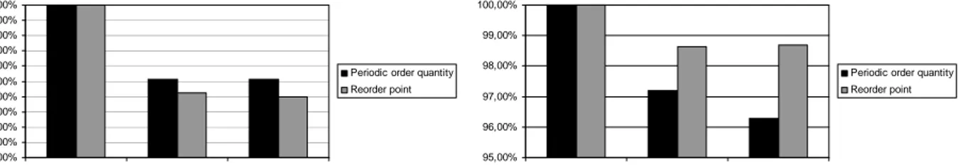
The forecast was fixed to reflect the yearly average in all three cases, meaning that the framework was bypassed to ensure that only the effect of seasonality on the methods would be measured. Ignoring safety stock altogether, the measures used for the simulations were fill rate and inventory cycle service level. Figure 5 shows the results for the three demand types.

Inventory cycle service level

0,00% 10,00% 20,00% 30,00% 40,00% 50,00% 60,00% 70,00% 80,00% 90,00% 100,00% 1 2 3 Simulation no.

Periodic order quantity Reorder point Fill rate 95,00% 96,00% 97,00% 98,00% 99,00% 100,00% 1 2 3 Simulation no.

Periodic order quantity Reorder point

Figure 5. Cycle service levels and fill rates.

What can be seen is that inventory cycle service is higher for the periodic order quantity method, while the reorder point method has a higher degree of inventory cycles with stock-out. However, the fill rate shows that the reorder point method is the best at fulfilling demand. Together, the measures tell that the periodic order quantity method has fewer, but significantly greater stock-outs than the reorder point method. Seasonality affects the severity of the stock-outs for the periodic order quantity method, but not for the reorder point method, which manages the variations in demand by shortening the inventory cycle time. We may therefore conclude that seasonality can have a noticeable effect on methods that are not designed for such demand patterns.

In contrast with the above simulations, the one which used information from the case company was based on the framework, integrating forecasts and inventory control methods. The result of the simulation is shown in Figure 6, which is based on fill rate and the total yearly cost of the inventory policy. The periodic order quantity system shows a considerably worse fill rate than the reorder point system, though the safety stock is sized so that both methods should have the same fill rate if demand were non-seasonal.

Periodic order quantity

Reorder point

Figure 6. Total inventory costs and fill rates.

7.DISCUSSION

The simulations indicate that the fill rate of the periodic order quantity method suffers when a seasonal demand pattern is introduced, while the reorder point method can maintain the same fill rate as if no seasonality were present. This is a result of the nature of the two methods, where variability affecting the reorder point method will affect the time of ordering, while the periodic order quantity method, with fixed ordering times, cannot regulate order timing to prevent stock outs. Instead, it must let the inventory level take the full effect of any variability. Conversely, the effect of variability on the reorder point method is that the resulting order interval may not be economic. Uneconomic order quantities are not always a severe problem, as shown by Axsäter’s investigation of less-than-optimal order quantities.

When comparing the methods used in the timber yard simulation using the framework, we find that the reorder point method is superior both concerning the safety stock costs, and the fill rate. The extremely low fill rate (77%) demonstrated by the periodic order quantity shows how inventory control methods that are unsuitable for the planning environment can be affected. The use of a monthly forecast not representing the next inventory cycle may also have contributed to the low fill rate. The simulation based on the framework helped give insight into how the inventory control process would react to the planning environment. It showed that a large safety stock would be required if the periodic order quantity were to be used. If applied over multiple products, the framework can tell if consolidation using the sensitive periodic order quantity system is less costly than the insensitive reorder point system. Given that the periodic order quantity system has a 100% uncertain time [1], it may be used as a benchmark in simulations, as variability and problems caused by poor design of the process always will be reflected in the fill rate. This means that efforts to improve an inventory control process can be tested using this method.

In the future we are planning to enlarge our simulation experiments by incorporating different kind of demand types (continuous and discontinuous) as well as new methods used in forecasting and ordering. Recent research works have shown that autoregressive and particularly GARCH forecasting methods outperform others in situations, where demand is fluctuating widely and has clearly “life-cycle” pattern [11]. Similarly recent purchasing order method research has argued that not a single ordering method should be used (so basically it is not a question, which method is the best one, but which one is most suited to certain environment), but usually combination of different purchasing methods should be incorporated in ERP systems during the entire life-cycle of a product [12]. However, if volumes are low, then even economic order quantities/reorder point systems, and periodic order policies should be abandoned; lot for lot policy might produce best results in these situations [12]. Thus, much depends from the operations strategy (order or stock based system), and from the amount of time, which customers are willing to wait for a delivery to reach their facilities [13].

8. CONCLUSIONS

Treating inventory control and forecasting as separate activities, while not acknowledging how forecasting and its application may affect inventory control may lead to incorrect assessments of a system’s performance in a certain planning environment. Approaching inventory control as a process that starts with a planning environment and ends with a measurement of the system’s performance shows that all activities are related, and that the end result may be

affected by the activities or by the way they are connected. In this paper a simulation model was built, to show how the framework could be implemented, and simulations were run. It was shown, that using the framework to design an inventory control process enables different systems to be compared, and gives measures of how a complete inventory control process performs. Using the framework to design simulation models for testing a system for a planning environment will give a clearer view of how the system will react, than if forecasts and inventory control methods were evaluated alone. Describing the activities and the connections presented in the framework gives a complete system that may be implemented exactly as described. Documenting a system in this manner, enables transfer from simulation models to real inventory control applications or vice versa. Using simulation models to evaluate changes to the planning environment, or a change in the methods used is also easily done, due to the modular design of the framework.

REFERENCES

[1] S. Axsäter: Lagerstyrning, Studentlitteratur, Lund, Sweden, 1991.

[2] S. A. Mattsson: Logistikens termer och begrepp, PLAN, Stockholm, Sweden, 2004.

[3] S. A. Mattsson, and P. Jonsson: Produktionslogistik, Studentlitteratur, Lund, Sweden, 2003. [4] D. Waters: Inventory Control and Management, Wiley, Hoboken, U.S.A., 2003.

[5] S. Axsäter: Inventory Control, Springer, New York, U.S.A., 2006.

[6] T. E. Vollman, W. L. Berry, D. C. Whybark, and F. R. Jacobs: Manufacturing Planning and Control for Supply Chain Management, McGraw-Hill, New York, U.S.A., 2004.

[7] J. C. Higgins: Information systems for planning and control: concepts and cases, Edward Arnold, London, United Kingdom, 1976.

[8] W. R. Ashby: An Introduction to Cybernetics, Chapman & Hall, London, United Kingdom, 1957. [9] M. Pidd: Computer Simulation in Management Science, Wiley, Hoboken, U.S.A., 1988.

[10] S. A. Mattsson: “Inventory control in environments with short lead times”, International Journal of Physical Distribution & Logistics Management, Vol.37, No.2, pp.115-130, 2007.

[11] S. Datta, C. W. J. Granger, D. P. Graham, N. Sagar, P. Doody, R. Slone, and O.‐P. Hilmola: “Forecasting and risk analysis in supply chain management – GARCH Proof of Concept”, MIT Forum for Supply Chain Innovation, ESD‐CEE,

School of Engineering. Available at URL:http://dspace.mit.edu/bitstream/handle/1721.1/43943/GARCH%20Proof%20of%20Concept%20_%20Datta_Granger

_Graham_Sagar_Doody_Slone_Hilmola_%202008_December.pdf?sequence=1. Retrieved: January 2009.

[12] O.-P. Hilmola, H. Ma, and S. Datta: “A portfolio approach for purchasing systems: Impact of switching point”, Massachusetts Institute of Technology, Engineering Systems Division Working Paper Series, ESD-WP-2008-07. Available at URL: http://esd.mit.edu/WPS/2008/esd-wp-2008-07.pdf. Retrieved: January 2009.

[13] P. Hilletofth: “Differentiated Supply Chain Strategy – Response to a Fragmented and Complex Market”, Licentiate dissertation, Chalmers University of Technology, Department of Technology Management and Economics, Division of Logistics and Transportation, Göteborg, Sweden, 2008.