THESIS
AN ANALYSIS OF HOUSING VALUES AND NATIONAL FLOOD INSURANCE REFORM UNDER THE BIGGERT-WATERS ACT OF 2012
Submitted by Daniel Clark Villar
Department of Agricultural and Resource Economics
In partial fulfillment of the requirements For the Degree of Master of Science
Colorado State University Fort Collins, Colorado
Fall 2015
Master’s Committee:
Advisor: Christopher Goemans Jordan Suter
Copyright by Daniel Clark Villar 2015 All Rights Reserved
ABSTRACT
AN ANALYSIS OF HOUSING VALUES AND NATIONAL FLOOD INSURANCE REFORM UNDER THE BIGGERT-WATERS ACT OF 2012
Previous research has shown that both flood risk and insurance premiums are capitalized in housing values. This paper examines the effect of National Flood Insurance Program reform implemented by the Biggert Waters Act of 2012 and the Homeowners Flood Insurance
Affordability Act of 2014 on housing values over a three-and-a-half year time period. It is hypothesized that the effects of increasing flood insurance rates through the elimination of established subsidies was capitalized in home values resulting in a loss of value in areas where subsidies are maintained. The paper presents a hedonic price difference-in-difference OLS model which is then tested for flexibility to the policy period and robustness to the treatment group. The evidence indicates that (1) housing values trend differently for areas with subsidies than areas without and (2) that this effect is correlated with flood insurance reform periods and robust to the definition of the treatment group. I conclude that the Biggert-Waters Act had a negative impact on median home values for areas with subsidized policies.
ACKNOWLEDGEMENTS
First I would like to thank my advisor Prof. Chris Goemans for his insightful comments and suggestions including the presentation of tough questions that helped me form a more cohesive thesis. Without his guidance the research process would have been much less efficient and complete. I would also like to thank the rest of my thesis committee: Prof. Jordan Suter and Prof. Sammy Zahran, who also provided excellent feedback which has allowed me to complete a more comprehensive analysis than I would have realized on my own. Together my committee provided encouragement and motivation as well as a much needed critical eye that helped me to conduct my research in a way that was neither apprehensive nor presumptuous.
I would also like to thank Prof. Andy Seidl whose guidance as advisor to my Research Assistantship provided me with the experience necessary to successfully approach this paper. Along with my committee the advice I received from him not only helped with this particular project but will be essential in future research endeavors; for the various strategies to approach a project and the critical lenses through which to view my own work I am extremely grateful.
My sincere thanks also goes to my fellow classmates for the thoughtful questions and good natured competition they directed my way. Without them this task would have been much less enjoyable. I would also like to thank Prof. Dale Manning for his comments on an early draft and everyone else who contributed to the development and writing of this thesis.
Last but certainly not least I would like to thank my family who provided moral and material support throughout the writing process: my parents, my sister and each of my grandmothers. Individually and collectively they endowed me with both the opportunity and ability to conduct this research in the first place. Their encouragement has been invaluable.
TABLE OF CONTENTS
ABSTRACT……… ii
ACKNOWLEDGEMENTS………iii
CHAPTER ONE: INTRODUCTION……….. 1
Goals and Structure of the Study………. 1
The National Flood Insurance Program: From Past to Present………3
A Review of Prior Research ………10
CHAPTER TWO: METHOGOLOGY……….. 13
Identification Strategy ………13
CHAPTER THREE: DATA AND CONTEXT ………16
Real Estate Data ……….16
Flood Insurance Data ………20
Additional Data ………..24
CHAPTER FOUR: RESULTS ………..30
Basic Models ………....31
Robustness of the Trend: Monthly Treatment Periods ………..34
Robustness of the Trend: AR(1) Dependent Lag Specification……….40
Robustness of the Trend: First-Order Error Autocorrelation ……….43
Robustness of the Trend: Spatial Error Model ………..45
Robustness of the Treatment: Random Treatment Group Membership ………47
Robustness of the Treatment: Housing Recovery ………..49
Robustness of the Treatment: Coastal vs Non-Coastal ………..51
Robustness of the Treatment: Age of Housing Stock ………53
Robustness of the Treatment: Quantiles ………55
CHAPTER FIVE: CONCLUSIONS ……….59
REFERENCES ………..62
APPENDIX I: STATIONARITY ………..66
CHAPTER ONE INTRODUCTION
Goals and Structure of the Study
This paper considers recent reform of the National Flood Insurance Program (NFIP) under the Biggert Waters Act of 2012 (BW12). The “Big Question” this paper aims to answer is whether changes in the administration of insurance premium subsidies had a measurable effect on residential housing markets across the United States. The NFIP has over 5.6 million policies, almost one for every twenty households across the U.S. With the implementation of BW12 in January and October 2013 the reform measures effectively increased the rates of property owners who received subsidized NFIP premiums. Whether subsidies were eliminated or substantially reduced and when these changes took place depended upon the type of property covered; however, all subsidized policies were affected by the reform. Later, in March 2014, these measures were scaled back due to popular recall of BW12. The passage of the Homeowners Flood Insurance Affordability Act of 2014 (HFIAA) renegotiated the terms of subsidy phase out period and reestablished some subsidies resulting in refunds to property owners who overpaid.
The main goal of the paper is to assess the difference in median home values between those zip codes directly impacted by the policy and those not directly impacted by analyzing home values in all time periods before, during and after implementation of BW12. This is done by applying a basic difference-in-differences model to a panel of median home values from January 2010 to May 2015. Anecdotal evidence found in places as diverse as local news media reports and official testimony at congressional hearings has implied that uncertainty surrounding both the expected ex-ante magnitude of these changes and the ex-post realization of increased
insurance premiums slowed or stalled housing markets in areas with a substantial number of subsidized structures.1 The economic rationality for an observable change in home values around reform implementation posits that as the expense of homeownership for a particular structure rises its transaction value will decrease by the same or similar amount in order to maintain a consistent net value of the property. An alternative but not mutually exclusive theory is that an increase in insurance premiums could lower housing values because it signals greater flood risk to the market. Either drop in property values could be restated as a reduction in land rents due to the increased internalization of flood risk. The primary aim of this paper is to determine if the increase in the effective NFIP flood insurance premium resulted in decreases in median home values according to this logic, though it may not be possible to tell which theory is the leading factor.
This paper is comprised of five chapters. The first chapter presents an introduction to the study, the National Flood Insurance Program and previous research. Chapter Two introduces the basic methodology. The data used in the study is presented in Chapter Three along with a general strategy for overcoming empirical estimation issues. Chapter Four presents results of the
established model, several modifications and robustness tests of both the identified trend and to alternate causal explanations. The final chapter concludes the study by summarizing the findings and suggesting areas for future research.
1 See the testimony of Donna Smith in Insuring Our Future: Building a Flood Insurance Program That We Can Live With, Grow With and Prosper With: Hearings before the Committee on Appropriations Subcommittee on
The National Flood Insurance Program: From Past to Present
The National Flood Insurance Program (NFIP) was established in 1968 as a flood insurance program underwritten by the Federal Government and operated by the Federal Emergency Management Agency (FEMA). The NFIP is intended to support the provision of flood insurance in areas that private insurers are unwilling to offer coverage. The necessity of expanding flood insurance coverage became apparent after Hurricane Betsy triggered massive uninsured losses in the Gulf of Mexico in 1965. In order for home and business owners or renters to be eligible to receive flood insurance their communities must participate in the program. Participation requires communities to engage in flood mitigation and loss reduction efforts that meet or exceed FEMA requirements.2 In theory this leads to a win-win situation whereby communities reduce the risk of catastrophic flooding, insurers lessen their exposure to covered losses and the Federal Government reduces the need to rely on taxpayers for emergency
assistance. Today, policies are administered either directly by FEMA or by property and casualty
insurers who participate in the “Write Your Own” Program.3
Subsidies were not a prevalent part of the original NFIP but were expanded a few years after its inception. The intent was that by lessoning the financial impact on property owners the program would be more appealing to community members. These subsidies were not means tested and instead were offered to the owner of any structure that was already standing when it was drawn into a federally designated flood zone by a new federal Flood Insurance Rate Map
2 According to the Government Accountability Office such efforts include diverting the flow of water through well-designed channels and retaining walls, or by containing the water through ponds GAO, . It is also worth noting the existence of the Community Rating System, which is a voluntary incentive program offered to communities that exceed the minimum requirements of the NFIP, also offers reduced rates but these are not considered to be subsidized.
3 The Write Your Own program allows private insurers to issue policies underwritten by the Federal Government in exchange for an expense allowance.
(FIRM). The expectation at the time was that the stock of subsidized properties would decrease as structures reached the end of their useful life; however, this has taken longer than expected and nearly a quarter of property owners with NFIP policies still receive subsidized insurance premiums (American Rivers, 2011).4
A second round of widespread uninsured losses after Hurricane Agnes in 1972
demonstrated that the first formulation of the NFIP had failed to adequately provide sufficient flood insurance coverage. In 1975 the federal government began requiring participation in the NFIP to receive federal disaster assistance and federally backed mortgages in flood plains to incentivize communities to participate in the program. These provisions stand today and flood insurance is required for any structure located in a high risk area with a federally backed mortgage. Structures in low risk areas are typically not required to carry flood insurance, although lenders can require flood insurance at their discretion. Because private insurers are typically unwilling to underwrite their own flood risk, alternatives to FEMA underwritten policies are difficult to locate.5 For FEMA underwritten policies, calculation of insurance premiums is complex and depends on several factors including the type of structure insured, the choice of content coverage and deductibles, as well as the designated base flood elevation. Properties that continue to receive a subsidy are a diverse mixture of pre-FIRM residences, businesses, non-primary residences and properties that have experienced severe repetitive loses as well as any structure grandfathered into a new flood zone.Pre-FIRM properties are all properties that have not been sold, significantly remodeled or rated with elevation data since the
4According to the Government Accountability Office, as communities were mapped and joined NF)P, new subsidized policies were added. While the percentage of subsidized policies has decreased since the program was established, the number of these policies has stayed fairly constant GAO, .
NFIP was reformed in 1974. 6 All subsidized properties were affected in some way by the reduction in subsidies under BW12. Some nonsubsidized policies saw their rates reduced as true risk was reassessed.
In addition to offering subsidized premiums, the NFIP calculation of rates is only meant to cover the average historical loss year. That the NFIP was never designed to deal with extreme events without assistance has brought insurance reform back into the political arena. Both of these practices resulted in NFIP premiums that are generally lower than if they were structured to insure against the true risk levels associated with flood hazards. This has left the program
vulnerable to natural variation in the severity of extreme events.
The extensive destruction caused by Hurricanes Katrina, Rita and Wilma in 2005 resulted in the NFIP facing a deficit of over $19 billion; a shortfall the program is unlikely ever to recover without a taxpayer bailout (Holladay and Schwartz 2010). Compounding this issue is that FEMA has excluded 2005 as an outlier in the calculation of the average historical loss year moving forward to avoid popular outcry from what would be large across the board increases. However, a solution was needed to avoid reliance on taxpayer support for Katrina and future catastrophes and to maintain the viability of the NFIP. The first signs of a serious movement for flood insurance reform surfaced in the summer of 2011 when the Senate banking committee drafted legislation which authorized the phase-out of NFIP subsidies and a bill was passed by the House of Representatives calling for reform in a 406-22 vote. 7
6 Some of the most common mitigation strategies for residential buildings that would be considered a significant remodeling effort include elevating a building to or above the area’s base flood elevation, relocating the building to an area of lower flood risk, or demolishing the building and turning the property into green space GAO, .
7See Senate Banking Committee NFIP Bill Forgives Debt, Reforms FEMA Role on PropertyCasualty available at http://www.propertycasualty360.com/2011/07/18/senate-banking-committee-nfip-bill-forgives-debt-r and published on July , and Special report: Irene wallops flood insurance program available at http://www.reuters.com/article/2011/08/31/us-storm-irene-flood-idUSTRE77T5M620110831
In order to place the burden of flood damages on those bearing flood risk Congress passed the Biggert-Waters Act of 2012 on July 6. Among other provisions the law mandated the elimination of subsidies in order to bring all insurance policies in line with actuarially defined
“true-risk” rates. The implementation of full-risk rates began in January of 2013 with
single-family non-principal residences and was extended to all other subsidized policies in October 2013. True-risk rates were charged either immediately upon the realization of certain triggers or phased in at an annual increase of 25% until full risk rates were reached, depending on the type of structure and policy held. Table 1.1 describes each policy type and the effect of BW12 on its insurance premium.
Table 1.1: Summary of Policy Types and Impact of Biggert Waters Policy
Code
Policy/Property Description Effect of BW12 Effective Date
A Any property sold and policies lapsed or new since enactment
Full risk rated on renewal 10/1/2013
B Single-family non-principal residences
25% increase in premium rates each year until premiums reflect full risk rates
1/1/2013
C Business non-residential 25% increase in premium rates each year until premiums reflect full risk rates
10/1/2013
D SRL Pre-FIRM subsidized 25% increase in premium rates each year until premiums reflect full risk rates
10/1/2013
E Single-family or condo unit principal residences
Full risk rated on sale, lapse, or SRL 10/1/2013
G Two to four family Full risk rated on sale, lapse, or SRL 10/1/2013 H Five or more family Full risk rated on sale, lapse, or SRL 10/1/2013 I Condominium building Full risk rated on sale, lapse, or SRL 10/1/2013
F Non-pre-FIRM SRL Non-subsidized N/A
K All others Non-subsidized N/A
The effect of this policy was estimated to increase the aggregate premium across all NFIP policies by 50% to 75%, while keeping unaffected policies unchanged (Hayes and Neal, 2011). However, since the roughly 1.1 million subsidized policies affected by the law make up only
20% of the program, the burden of this substantial increase is heavily concentrated on a small proportion of policies. Based on the 2012 statistics this constitutes a net increase in premiums earned of $1,670,667,881 to $2,506,001,822, or an average increase of up to $2,278 in annual premium for each subsidized policy.8 Given the substantial variation in policy coverage options and risk exposure, reported increases in annual premiums of up to $35,000 are not entirely unbelievable.
On January 1, 2013 the new rates began to be levied on the roughly 1.1 million policies affected by the new law. Initially, only homeowners with subsidized insurance rates on non-primary residences. On October 1, 2013 the provisions covering all subsidized properties took effect. Shortly afterwards the states that saw the greatest impact began experiencing political backlash. In the summer of 2013 Maxine Waters, one of the laws namesakes, spoke against the dramatic rate increase and soon after, along with twenty-six other congressional leaders, wrote to Congress in protest of the way BW12 had been implemented and called for changes to the bill.9 Louisiana led efforts to have the provisions of BW12 modified or recalled. On January 30, 2014 the Senate passed a bill to delay certain flood insurance rate hikes and on March 21 the
Homeowners Flood Insurance Affordability Act of 2014 (HFIAA) was signed into law by President Barak Obama. A summary of important flood insurance reform events is given in Table 1.2. The new legislation reduced the rate at which premiums would reach full-risk pricing but did not eliminate the move to full risk rates. Under HFIAA annual rate increases are capped
8 These estimates are based on the 2012 Total Earned Premium of $3,342,335,762 (FEMA, 2015) and the findings of Hayes and Neal (2011).
9See Waters vows action to avert 'unaffordable' premium hikes blamed on flood insurance bill available at http://www.nola.com/politics/index.ssf/2013/05/co-author_of_flood_insurance_a.html and Congressional letter asks FEMA to administratively block huge flood insurance hikes available at
http://www.nola.com/politics/index.ssf/2013/07/congressional_letter_asks_fema.html published in May and July of 2013, respectively by the by NOLA Media Group.
at 5% - 15% of the full risk premium and an individual annual cap of 18% was imposed. HFIAA also removed the sale of a property as a trigger for subsidy loss due in part to reports that it had frozen real estate markets in flood hazard areas.10 While properties that fall into this category are exempt from rate increases under HFIAA, they initially faced the same provisions as all
subsidized properties under BW12 so are included in the study. Furthermore, it is not
unreasonable that they could expect to face some sort of rate increases in the future. In general, policy makers are likely to continue to pursue flood insurance reform due to increases in coastal development and changes in flood risk associated with climate change, making reform an area ripe for continuing study.
Table 1.2: Summary of Major Events
Date Event
May 1957 American Insurance Association Study states that private industry cannot provide flood insurance because only those at highest risk buy it
September 1965 Hurricane Betsy prompts the establishment of the NFIP in 1968.
December 1974 Prompted by Hurricane Agnes Congress makes flood insurance mandatory for certain federal programs
July 1983 FEMA begins allowing private insurers to write flood insurance policies underwritten by the Federal Government.
August 29, 2005 Hurricane Katrina makes landfall in Louisiana, catalyzing serious debate on reforming the National Flood Insurance Program.
March 16, 2006 Congress begins an effort to investigate the National Flood Insurance Program with a series of Flood Insurance Reform and Modernization Acts beginning with H.R.4973 April 22, 2010 With the beginning of the great recession flood insurance is left off the congressional
legislative effort until the introduction of H.R.5114 - Flood Insurance Reform Priorities Act
July 2011 The Senate and the House each move in support of flood insurance reform.
• The Senate Banking Committee approves FEMA debt forgiveness and mandates phase out of subsidies
• The House votes 406-22 in favor of flood insurance reform. April 16, 2012 The Biggert-Waters Act of 2012 is introduced (H.R. 4348)
July 6, 2012 The Biggert-Waters Act of 2012 is signed into law • Reauthorized the NFIP for 5-years
• Introduced rate and map making reform measures
January 1, 2013 Premiums are increased 25 percent each year until reaching full-risk rates for: • Non-primary residences
March 19, 2013 Congress begins to reassess the reform measures implemented under Biggert-Waters when the Flood Insurance Premium Relief Act (H.R.1267) and Flood Mitigation Expense Relief Act (H.R.1268) are introduced.
June 2013 The U.S. House of Representatives passes a bill that would delay rate hikes 281 -14611 October 1, 2013 Premiums are increased 25 percent each year until reaching full-risk rates for:
• Severe Repetitive Loss properties
• Properties with cumulative paid flood losses exceeding fair market value • Businesses/non-residential buildings
Full-risk rates take effect upon renewal for:
• Property purchased on or after July 6, 2012 • New policies effective on or after July 6, 2012
• Lapsed policies reinstated on or after October 4, 2012
October 29, 2013 The bill that would later become the Homeowner Flood Insurance Affordability Act of 2014 is introduced (H.R.3370).
A Review of Prior Research
Evidence for housing price differentials for properties located around hazards and the role of insurance premiums in housing markets has been acknowledged in the literature since at least the mid-1980’s (MacDonald, et al., 1990; MacDonald, Murdoch and White, 1987), while more recent research has continued to shed light on the subject. Bin, Kruse and Landry (2008) regress the log of home values on housing attributes and an indicator for flood risk using a pooled first-order spatial hedonic model and find evidence that flood risk information is conveyed to buyers in the coastal housing market through insurance premiums regardless of whether flood insurance is purchased or not. Their analysis suggests that housing markets adjust for flood risk signaled through flood insurance premiums on a neighborhood level, rather than by the characteristics of the individual structure. An implication of this is that changes in insurance premiums will affect entire neighborhoods, regardless of which structures are actually insured. The authors also indicate that pre- and post-FIRM properties are not valued differently, again suggesting that neighborhood level flood insurance signals overwhelm the structure-specific influence of age, the primary determinant of pre- and post-FIRM attributes. These results lend support to the idea that changes in flood insurance premiums may be capitalized by local housing markets and that a change in rates may lead to a measurable change in home values and indirectly support the idea that the effect of insurance changes on home values can be adequately measured on the
neighborhood or zip code level as put forth in this paper. I expand on these findings by looking at differences in the capitalization of flood insurance between zip codes before, during and after the insurance premium price changes associated with BW12. Evidence of a change in value will support the finding that the insurance premiums have an impact on the market value of a
property; though the mechanism for this could be the change in the cost of ownership itself, to the new level of risk it signals to the market or both.
Prior research has established a connection between flood risk or flood events and decreases in housing values. Daniel, Florax and Rietveld (2009) conduct a meta-analysis of studies across ten states in which they show that “an increase in the probability of flood risk of 0.01 in a year is associated with a difference in transaction price of an otherwise similar house of -0.6%” but does not identify whether the risk or insurance was the causal factor. In another study Bin and Landry (2013) identify temporary but significant decreases in housing values due to flood risk perception. Using a difference-in-difference framework they show increases in risk premiums for homes sold in and around the flood plains of Pitt County, North Carolina after Hurricane Fran in 1996 and Hurricane Floyd in 1999. They find that the value for flood-zoned properties decreased by 5.7% to 8.8% after Hurricane Fran and 8.8% to 13% after Hurricane Floyd with an overall decrease of 6% to 20%, depending on model specification, while the risk premium itself diminishes over time and dissipates completely after six years. Most properties in the study area received little to no damage and robustness checks revealed that results were due to risk perceptions rather than significantly damaged properties.
Similarly, a study of Alachua County, Florida by Harrison, Smersh and Schwartz (2001) find that homes located in a flood zone sell for less than homes located outside of flood zones. Significantly, the price differential within the flood zone is less than the present value of future flood insurance premiums. An implication of this finding is that changes in the expected value of future flood insurance premiums may be partially muted in the housing market. As a result of partial capitalization in the housing market observed changes may be less than the amount of the premium increase. It follows that home values in areas with the largest price increases will be
most affected while areas with relatively small changes may not show measurable effects of the flood insurance reform.
Prior research has also explored the socioeconomic factors that contribute to flood vulnerability and NFIP participation with a general consensus that flood risk affects especially poor and especially rich counties due to the trade-off between amenities and flood risk.12 This distribution leads to a possible disproportionate effect of insurance reform and affordability concerns depending on who holds the subsidized policies in the NFIP program (Kousky et al. 2013). Additionally, research has suggested that state-level analysis of the insurance program can
“hide important local differences,” implying that investigation of the effects of BW12 on the zip
code level is a meaningful pursuit (Michel-Kerjan, 2010). Although this paper does not attempt to address the question of social equity, these findings motivate this study as they suggest that flood insurance reform could have substantial unintended consequences that have not been adequately addressed in the literature.
CHAPTER TWO METHODOLOGY
Identification Strategy
The basic mechanism by which an increase in flood insurance premiums realized through the reduction of NFIP subsidies may lead to changes in the median home value in a
neighborhood is captured by the general hedonic model �� = � , � , � , where �� is the median value of a home in neighborhood i in time t, � is a matrix of associated neighborhood specific location characteristics, � represents the structural characteristics of the median home in that area and � are market characteristics (Tu, 2005). The NFIP characteristics of a
neighborhood, such as the number of subsidies, belong to � while the policy that governs the subsidies may be considered a market characteristic.
The identification strategy for this analysis consists of utilizing dummy or indicator variables to estimate different effects of variables on median home values for zip codes
belonging to different groups. This is known as a difference-in-differences model. In the simplest terms the group identifier �� is regressed on y so that �� = + ��+ � ′� + �′� +
� ′� + �� where ��= indicates an estimate of �� from neighborhood i which belongs to
some group in time t and ��= indicates the neighborhood is not a member of the group in that period. The average effect on �� for a non-member is just while reveals the average difference in this value that membership imparts. Thus the equation yields two conditional estimates for ��� depending upon whether the neighborhood is a member of the group in time t:
��| ��= = + �′� + � ′� + � ′� when group membership is false and
Subtracting the former conditional expectation from the latter gives ; the difference in the conditional expectation of �� for positive group membership. Where the characteristic defining group membership is the presence of some condition the group is known as the treatment group. Since the total effect on the treatment group is relative to the total effect on the non-treatment group, the latter is referred to as the reference group when �� = .
The basic model begins by identifying two types of neighborhoods represented by the indicator �. Zip codes that are directly affected by the BW12 provisions on subsidized policies have subsidized NFIP policies in force and are represented by a positive indication,
� = , and zip codes that are not directly affected have some number of NFIP policies in
force, but none are subsidized, are identified by � = . The basic model also begins by
distinguishing three time periods that an estimate can come from. The first two policy periods are denoted with indicator variables. An estimate from the period between when BW12 was passed to its repeal is indicated by � = and the post repeal period is indicated by �= . The base period is the reference period, where both � and � are zero. Since all zip codes are always in the same time period these do not need to be distinguished by zip code. This model hypothesizes that some effect on housing markets occurred after passage and all the way through to repeal and is represented:
(Eq. 2.1)
�� = + �+ �+ �+ �∗ � + �∗ � + �� ′ + ��
where �� is a matrix containing the zip code attributes � , � and � .
In this framework and give the average difference in median home value during the treatment window and after the treatment period, respectively. The coefficient allows the marginal change in median home values to be different for zip codes directly affected by the
treatment from passage to repeal. This is expected to be negative if removing subsidies affected housing markets with subsidies different than those without. After BW12 is repealed the change in median home values for areas with subsidies, represented by , is expected to be less than if HFIAA was seen as a benefit to subsidized areas. This model does not control for estimation issues arising from panel data dimensions, which are discussed in the following section.
CHAPTER THREE DATA AND CONTEXT
This section describes the three main types of data used in the study, real estate data, flood insurance data and zip code characteristics. This study uses the series of recent flood insurance reforms of the Biggert-Waters Act and the Homeowners Flood Insurance Affordability Act to study the effect of flood insurance premiums on median home values. The primary
question up for investigation is whether a measurable change in property values is detectable before, during or after BW12 due to the changes in flood insurance subsidy administration. Data on home values is obtained from the Zillow Group while flood insurance information is provided by FEMA. This section also presents some of the short comings of the data and the assumptions necessary to utilize it for the study.
Real Estate Data
The dependent variable for the analysis is the median value of homes in a neighborhood. Data for the dependent variable comes from a collection of monthly time series of estimated median home values for a panel of zip codes. The values are estimated with proprietary statistical techniques by the Zillow Group and are accessible on their Real Estate Research website. The series is known as the Zillow Home Value Index (ZHVI) and is available at several geographic resolutions and for a variety of market segments. I utilize the ZHVI on the zip code level
covering all home categories including single family residences, co-ops and condominiums from January 2010 through May 2015. Zillow property value estimates in real estate research have appeared as both dependent and independent variables in peer reviewed and scholarly
publications.13 The ZHVI itself has also been the subject of study. While accuracy has been shown to vary there is a general consensus that it provides reasonably accurate estimates for an aggregate analysis of property values.14 Hagerty (2007) in particular found a 7.8% median margin of error in Zillow estimates that was not systematically under or over estimated. The accuracy of Zillow estimates was also shown to differ for outliers and less densely populated areas. Gelman et al. (2011) find user submitted information on Zillow improves completeness but is not always accurate.
The ZHVI provides estimates of median home value in order to provide data that is not influenced by the characteristics of the particular homes sold in a given period. This validates the assumption that median structural characteristics can be eliminated by mean-differencing. By tracking full-value, arms-length sales that are not foreclosure resales and applying machine learning techniques the ZHVI aims to provide consistent home value estimates. The index is estimated using the same set of homes in each period, thus keeping the sales mix constant across time, while allowing characteristics to vary across zip codes. Important housing attributes that are considered in the model include physical facts about the home and land such as structure type and number of rooms, prior sale transactions, tax assessment information and geographic
location. As an estimate, this data is subject to estimation error; however, Zillow assures that
there is minimal systematic error. In other words, the “error is just as likely to be above the
actual sale price of a home as below” (Zillow Real Estate Research, 2014). Other modifications
13 See Kay et al. (2014) and Huang and Tang (2012) for examples of peer reviewed literature and Garriga (2013), Qiao et al., Stratmann (2013), Frey et al. (2013), Morris-Levenson (2014), Keating (2014), Cronqvist and Yonker (2009) and Guerrieri et al. (2013) for scholarly articles.
14 See Kay et al. (2014) and Frey et al. (2013) for comparisons of Zillow data to actual sales in regression analysis; Hagerty (2007), Hollas et al. (2010) and MacDonald (2006) for accuracy of Zillow estimates; and Ma and Swinton (2012), Kim and Goldsmith (2009) and Clapp and Giaccotto (1992) for the use of assessed values in general.
of the data include the application of a five-term Henderson Moving Average Filter to reduce
“noise” and seasonal adjustments. The net result is a median home price index comparable
across both space and time. A graph of the average median home value across all zip codes reveals a strong upward trend in median home values is clearly visible beginning in March 2012 (Figure 3.1). Prior to that date median home values had been decreasing. The graph also includes the average change in median home values, revealing that the increase in median home values slowed considerably after August 2013, though the marginal growth rate remained positive. It is apparent from this graph that the trend in median home values over the course of this study changes over time.
Figure 3.1: Average Median Home Value and Average Change in Value across All Zip Codes
$152,000 $162,000 $172,000 $182,000 $192,000 $202,000 $212,000 $222,000 $232,000 $242,000 $252,000 -$2,500 -$2,000 -$1,500 -$1,000 -$500 $0 $500 $1,000 $1,500 $2,000 $2,500 Jan 1 0 M ar 1 0 M ay 1 0 Ju l1 0 S e p 1 0 N o v 1 0 Jan 1 1 M ar 1 1 M ay 1 1 Ju l1 1 S e p 1 1 N o v 1 1 Jan 1 2 M ar 1 2 M ay 1 2 Ju l1 2 S e p 1 2 N o v 1 2 Jan 1 3 M ar 1 3 M ay 1 3 Ju l1 3 S e p 1 3 N o v 1 3 Jan 1 4 M ar 1 4 M ay 1 4 Ju l1 4 S e p 1 4 N o v 1 4 Jan 1 5 M ar 1 5 M ay 1 5
Average ZHVI Statistics
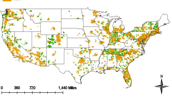
Overall, Zillow provides data for 24,460 zip codes while NFIP data is available for 33,144 including American territories such as Guam, Puerto Rico, the U.S. Virgin Islands and American Samoa. The total viable overlap of the two datasets is for 12,091 zip codes. Overall, much of the geographic area of the United States is not covered by this study but over 76% of the continental U.S. housing market is covered by population.15 The study covers primarily
metropolitan areas (Figure 3.2). As a result generalizations to rural areas may not be made with the same confidence as to metro areas.
Figure 3.2: Study Scope by Metro and Non-Metro Distinction
Flood Insurance Data
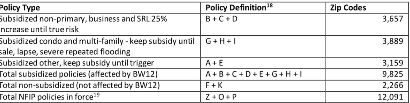
Data on the National Flood Insurance Programs policies in force comes from a cross-sectional dataset provided by FEMA.16 The dataset includes counts of total NFIP policies by zip code and total subsidized and unsubsidized policies for the month BW12 was passed. Subsidized policies are further classified by subsidy type allowing for the identification of how and when it would be affected by BW12. Only zip codes with data on both median home values from Zillow and flood insurance policies from FEMA were included in the study. A complete breakdown of how the zip codes are categorized is presented in Table 3.1.17
Table 3.1: Number of Zip Codes by Type Included in the Study
Policy Type Policy Definition18 Zip Codes
Subsidized non-primary, business and SRL 25% increase until true risk
B + C + D 3,657
Subsidized condo and multi-family - keep subsidy until sale, lapse, severe repeated flooding
G + H + I 3,889
Subsidized other, keep subsidy until trigger A + E 3,159
Total subsidized policies (affected by BW12) A + B + C + D + E + G + H + I 9,825
Total non-subsidized (not affected by BW12) F + K 2,266
Total NFIP policies in force19 Z + O + P 12,091
While the majority of NFIP policies are concentrated in Florida, Louisiana, Texas and New Jersey, dividing the total number of policies in force by the total number of housing units in an area makes it apparent that the program is prevalent throughout the country and not j ust in coastal areas. Figure 3.4 illustrates the division by quantile. Areas in the top 20% of policies per
16 While some policy data with a time series component is available on the FEMA website detail needed for this study is not. A Freedom of Information Act request may be able to locate the desired information but was not feasible given the time constraints.
17 Only 2.5% of the data covered zip codes that did not participate in the NFIP at all, so they are excluded from the regression analysis as described in the methodology section. Also, 133 zip codes affected in January but not October are excluded so as not to have to control their influence in October. Since the 6,067 areas affected in January are the exact same type removing these shouldn’t affect the estimate. Additionally, zip codes are removed because of missing data on median home values.
18 These categories refer to the definitions presented in Table 1.1.
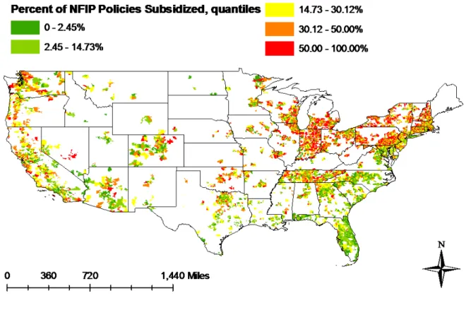
housing unit are scattered about the continental U.S. from Florida to Nebraska to Washington State. As previous studies have suggested, changes to the program are neither an exclusively coastal nor an exclusively metro issue. It is also apparent that the subsidies are distributed widely. Areas with the highest proportion of NFIP subsidized are all over the U.S., with some of the highest rates in the Great Lakes area (Figure 3.4).20 Florida has low rates of subsidies, despite having large numbers of subsidized policies in force, because of large numbers of NFIP policies in general. Simply having a large number of policies does not mean a low subsidy rate though, and vise versa; the correlation between these two measures is just -4%.
Figure 3.3: Policies in Force per 1,000 Housing Units
20 Note that this includes business policies under the National Flood Insurance Program so that the number of policies per housing unit could be greater than one.
Figure 3.4: Percent of Policies in Force with Subsidy
The use of a cross-sectional dataset in a time series analysis requires some potentially significant assumptions. If an unobserved change in policy data is correlated with explanatory variables, such as the treatment periods, and the value of a median home this would be captured by the error leading to a form of endogeneity bias caused by the omitted values of the NFIP series. Omitted variables may also lead to inefficient OLS estimation. The hypothesis of this study is that the number of policies is correlated with median home values and it is expected that the BW12 reforms impacted the values. For the impact of the omitted variables not to be
significant it must be assumed that the change in policy counts is not correlated with any of the included variables. This does not seem to be the case. Figure 3.5 shows how total policies in force have changed since 1990. The data indicate that policies in force increased until around
however a decrease can be seen around the time of BW12. It is reasonable to assume that
property owners maintaining voluntary NFIP policies may have dropped coverage in response to the policy. Thus the limited temporal dimension of the data likely induces an omitted variable problem.
Figure 3.5: Total Policies in Force over Time
It is assumed that a causal link exists between the reduction in policies in force and the BW12 reform leading to some omitted variable bias: as owners of subsidized structures realized the extent to which the loss of the subsidy would increase their premium some of those policy holders would elect to discontinue coverage. While this is an empirical question the data to assess this is not available. Addressing omitted variable bias requires the inclusion of the
variable or a closely related instrument and none was found. The question is now: how serious is this problem? It seems unlikely that whole communities would have elected to leave the program
0 1,000,000 2,000,000 3,000,000 4,000,000 5,000,000 6,000,000
Policies in Force
Policies in Forceentirely. I make the assumption that no zip codes changed group membership over the course of the study due to BW12 so that no bias exists when using indicators to represent zip code group membership.21 When using continuous measures of the number of policies in force the
unobserved change over time the reduction is due to mainly to those with subsidized NFIP
program dropping their policies. In this case the bias is expected to lead to underestimation of the effect of the treatment periods on median home values because of negative correlation between the number of subsidies and median home values during the treatment period. It is also expected to be relatively small; from 2011 to 2014 the total change in policies in force was roughly 5% with most of this change taking place from 2013 to 2014. While this is certainly not an
insignificant change, it is not extremely large.
Additional Data
It is assumed that certain location specific variables do not change significantly over the course of the study; however, the five year time period is long enough that this may not be accurate for some of these variables. Factors such as actual flood risk exposure, demographic composition, quality of schools, and access to natural amenities and political representation can change over time. Time invariant differences between zip codes can be captured with zip code specific fixed effects for variables that are time invariant by adding a zip code specific intercept
21 The boundaries of Flood Insurance Rate Maps could change over the study period and impact subsidies within a community but changes are made infrequently and new subsidized policy creation is assumed to be minimal. In general, map revisions are small and encompass areas considerably less than a zip code.
Additionally, one of the provisions of BW12 was to reassess and update FIRMs with new technology since so many were outdated and this process takes time. After reassessing flood risk the maps have to be drawn up and presented to the community for public debate and questioning. A 90-day appeal period is mandatory. Additional changes to premium rates under BW12 occur upon remapping, but the provision calling for these
� to the model, which may or may not be observed, and an associated individual specific error
term �, which is not. The general form of the model in equation 2.1 now becomes: (Eq. 3.1)
�� = � + + �+ � + �+ �∗ � + �∗ � + ��′
+ �+ ��
where �� is assumed to be an idiosyncratic observation-specific zero-mean random-error term. The total error term � + �� is subject to the OLS assumption that model errors are uncorrelated with the regressors for unbiased estimation of model parameters. Thus it is critically important that the unobserved individual error � is uncorrelated with any variable in the model. To remedy this problem a fixed-effects model applying mean differencing is utilized to remove the
heterogeneity effect and its associated error from the model. By doing so the time invariant heterogeneity parameters � − ̅ , � � − ̅ and � − ̅̅̅ , drop out of the equation.
Additional information on relevant neighborhood specific location characteristics and market characteristics are collected from various sources. The inclusion of structural
characteristics of the median home are not necessary because Zillow holds this constant.
Location specific attributes are both demographic and geographic. The latter attributes of interest include whether or not the zip code is coastal and the nature of flood risk in that area. While the flood zone ratings are generally available they must be accessed by individual community and stitched together. Since flood zones do not correspond to zip codes this was beyond the scope of available resources. Miles of rivers and stream, acres of lake and a coastal dummy are used to proxy flood risk. These measures provide insight into the type and quantity of risk faced. Since relatively large areas are able to contain larger bodies of water and more miles of river total square miles is included to control for the size of a zip code.
Demographic variables of interest fall into four broad categories: race, income, poverty and educational measures. Monthly series for these variables are not available. Local
demographic attributes of each zip code can be obtained on the zip code level from the U.S. Census Bureau 5-year American Community Survey for 2013. However, this dataset only
provides one cross-sectional estimate for the entire study period. As a result time variant location characteristics are not included in this study. Additionally, they cannot be assumed to be
uncorrelated with the regressors because they include time so omitted variable bias may be present if they determine median home values. Whether certain attributes vary significantly over the course of the study period is not clear but is an empirical issue. In short panel series
characteristics like the quality of education, demographic composition and political
representation can be thought of as constant. The longer the study the less this assumption may hold. It is expected that any bias is small for several reasons including the medium length study period. Because time trends will be accounted for general changes in location characteristics or how they affect median home values is important only in so far as they differ between zip codes. While this is likely, it is less hazardous to assume that changes differ between groups of zip codes. Participation in the NFIP program is voluntary so the study only compares areas that participate in the program. While what areas have and do not have subsidies are not necessarily random there is no direct selection into the group so correlation between group membership and unobserved location characteristics may not be large.22 Finally, the collinearity of time variant
22Receiving subsidies was not a voluntary option selected by communities but depended on when the area began the program and how recently homes have been drawn into a new flood plain. An indirect selection bias based on factors that contributed to early participation may be present, but for many communities receiving subsidies the initial F)RM would have been adopted in the ’s and ’s so time variant factors that would have contributed to initial participation would likely be different today. A characteristic such as flood risk exposure may lead to early participation. )t’s variability over time is not clear. The drawing of new
and time invariant location characteristics or any other included variable would diminish this bias. Ultimately none of these arguments refute the presence of endogeneity due to location characteristics that change over time and future research may include some measures of these.
Market characteristics are captured by the monthly average of the S&P500 Index. Additional market conditions common for all areas are captured by a monthly fixed effect �� which is a month specific intercept that measures the common difference in median home values across all zip codes in month t. To address unobserved differences over time within each zip code cluster robust standard errors are reported for all results when available. The robust
standard errors relax the assumption that observations within a group are independent and allows limited autocorrelation of errors within each area.
A visual inspection of average median housing values in Figure 3.1 clearly shows the presence of a general upward trend over time. Tests reveal that the series is deterministic, or has a unit root, meaning that there is a nearly one-to-one relationship between �� and �,�− . A unit root results in inefficient estimation of the model and the solution to this problem is to difference the series by its previous value.23 While a visible trend remains in the first differenced trend line the difference is found to be stationary.
An additional dimension not unique to panel data is space. To assess how the two areas differ within a difference-in-differences framework the assumption that the housing markets in each group are independent and that housing trends are similar is required. In regards to the issue of independence this may not always be the case. Because zip codes tend to be small housing
23 Most previous literature using Zillow estimates has used a log transformation; however, these studies often pool values from different years or consider a very short time period. See Kayet al. (2014), Stratmann (2013), Fret et al. (2013), Keating (2014) for log transformations. Morris-Levenson (2014) use the change in city level ZHVI as a dependent variable while Morris-Levenson (2014) uses the change in ZHVI, but as a dependent variable. See Appendix I: Stationarity for a discussion on this result.
values in one zip code may have direct or indirect effects on the housing values of nearby areas. Theoretically, spatial autocorrelation in housing markets may arise from two sources: common neighborhood characteristics that cast influence across subject boundaries and spatial spillover of housing prices between neighbors (Can, 1992). For example, zip codes may share the same school district, county services and local amenities that would exert a similar influence on median home values in separate but nearby locations. Additionally, nearby areas could serve as substitutes for one another resulting in a convergence of value across borders.24 Correcting for spatial lags or spatial errors can lead to improvements in parameter estimation over standard OLS; a few studies that have done so have favored the spatial error model more often than not. 25 Data descriptions and summaries for all variables are presented in Table 3.2 and Table 3.3, respectively.
24 If the nature of these spillovers are correlated with group membership this would introduce an omitted variable problem. Therefore in the absence of spatial econometrics it is necessary to assume spillovers are present for both groups and do not depend on group membership.
Table 3.2: Summary of Variable Definitions
VARIABLES DESCRIPTION
Dependent Variables
�� Zillow estimated median home values for zip code i in time t.
∆ �� The first-difference of �� Dependent Variables
� Total number of NFIP policies in force in zip code i in in July 2013.
� Total number of subsidized NFIP policies in force in zip code i in in July 2013. � Indicator equal to one if zip code i had subsidized policies in force in July, 2013; 0
otherwise.
� Indicator equal to one if the estimate is from the pre-enactment phase of Biggert
Waters: July, 2012 to January, 2013; 0 otherwise.
� Indicator equal to one if the estimate is from the entire Biggert-Waters period from
passage to repeal: July, 2012 to April, 2014; 0 otherwise.
� Indicator equal to one if the estimate is from the first enactment period of
Biggert-Waters provisions: January 2013 to March 2014; 0 otherwise.
� Indicator equal to one if the estimate is from the post repeal period of Biggert-Waters,
also the time the Homeowners Flood Insurance Affordability Act was in place: April, 2014 to May, 2015; 0 otherwise.
� The average value of the S&P500 Index for month t.
� Total housing units in zip code i in the 2013 5-year American Community Survey. � Median year built for the homes in zip code i.
� Indicator equal to one if zip code I is coastal, zero otherwise.
� � Miles of rivers and streams in zip code i � Land area of zip code I in square miles
� Indicator equal to one if zip code i was considered a metro area by the 2013 Rural
Urban Influence Continuum; 0 otherwise.
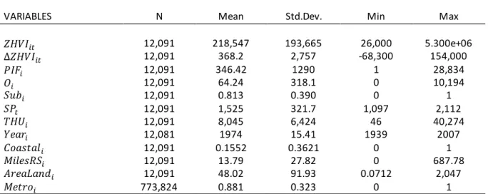
Table 3.3: Summary of Variable Statistics
VARIABLES N Mean Std.Dev. Min Max
�� 12,091 218,547 193,665 26,000 5.300e+06 ∆ �� 12,091 368.2 2,757 -68,300 154,000 � 12,091 346.42 1290 1 28,834 � 12,091 64.24 318.1 0 10,194 � 12,091 0.813 0.390 0 1 � 12,091 1,525 321.7 1,097 2,112 � 12,091 8,045 6,424 46 40,274 � 12,081 1974 15.41 1939 2007 � 12,091 0.1552 0.3621 0 1 � � 12,091 13.79 27.82 0 687.78 � 12,091 48.02 91.93 0.0712 2,047 � 773,824 0.881 0.323 0 1
CHAPTER FOUR RESULTS
This study aims to address whether flood insurance reform, specifically the Biggert-Waters Act of 2012, had a measurable impact on housing values. This section presents a series of models and results to test the robustness of each model to alternate specifications.26 The first section addresses Research Question 1 which attempts to identify if a difference in trend between areas with and without subsidies exists. The first subsection of section one presents two models using indicator variables for membership into policy participation groups and treatment periods; the second presents a more flexible analysis of the treatment period; subsection three accounts for robustness to an alternate order dependent lag model; subsection four accounts for first-order autocorrelation of the error process; finally, subsection five accounts for spatial correlation of the errors. The second question concerns whether this effect is unique to the definition of the treatment group or if alternate specifications produce similar results. The first section of section two randomly specifies membership to the treatment group, the second removes the four states affects the most by the real estate collapse, a coastal distinction is drawn third, the fourth subsection considers the median age of the housing stock and finally results are presented for low, mid and high quantiles of subsidy measures.
Research Question 1: Is there a difference in median home values between areas with and without subsidies associated with changes in the National Flood Insurance Program?
Basic Models
So far this study has identified two types of zip codes, areas that participate in the NFIP with and without subsidized policies in force, and three time periods, before passage, from passage to repeal, and after repeal. This section provides results for this model as well as an alternate specification of the time periods. In each model the reference group are areas that have no subsidized NFIP policies in force. This group serves as control group for the effect of the policy because it is not directly affected by the new conditions governing subsidized rates. The treatment group are zip codes that contain some number of subsidized NFIP policies; they are directly affected by BW12s subsidy provisions. The model that has been presented so far is reproduced in its entirety as Equation 4.1 and will be referred to as Model I.
(Eq. 4.1)
∆ �� = � + ��+ + �+ � + �+ � ∗ � +
�∗ � + ��′ + � + ��
Model I expresses the change in the median estimated home value of zip code i in month t as a function of policy variables, treatment periods, location specific characteristics, market conditions and monthly �� and individual � fixed effects. The time invariant variables, noted by the absence of a t subscript, will drop out during mean-differenced estimation. The coefficients of interest are and . The former measures the average difference in the change in median home values for zip codes that had subsidized policies in force in July 2013 during the period from passage in that month to repeal in April 2014.27 If the provisions on subsidies in BW12 had an effect on median home values this coefficient is expected to be significant. Specifically, it is expected to be negative. This would reflect that the change in median home
values over this period was on average less than that in areas without subsidies. For the expectation is less clear. If it is negative it would reflect that subsidized areas still had a rate of change in median home values below that of areas without subsidies. It is expected that the elimination of BW12 is a benefit, but it is not clear that that the Homeowners Flood Insurance Affordability Act is also a benefit or simply less of a bad thing. If the latter this coefficient will still be negative but should be greater than , if the former it may be insignificant or postivie.
Model II is represented by equation 4.2 and expands on Model I by allowing the period before enactment but after passage to be uniquely defined. This is done by dividing � into two parts. The first part is the period from passage to enactment ( �) and the second part is the entire period that BW12 was in effect ( �).
(Eq. 4.2)
∆ �� = � + ��+ + �+ �+ �+ �+ � ∗ �
+ �∗ � + �∗ � + ��′ + � + ��
The coefficient on the interaction between � and � has a similar interpretation to its interaction with � in Model I except that it specifically defines the period in which the BW12 provisions are in place. The coefficient on the � interaction is expected to be negative if the effects of the BW12 provisions were anticipated in areas with subsidies in place prior to enactment and insignificant otherwise.
Results for Models I and II and are presented in Table 4.1. Before examining the coefficients of interest it is worth nothing that the coefficients on the treatment period are positive and significant.28 The positive sign indicates an increase in the change in median home
28 To test the robustness of the models to the specification of the time effect these models were run with continuous time variables instead of fixed effects. Polynomials up to order five were included. All time trends were significant and the treatment periods remained significant in each of the new specifications although the
values over these periods. Their interaction with the subsidy group indicator is consistent in all models. Each one shows that the change median home values in was less in every period, including the pre-enactment and post-repeal phases. The differences between all treatment and group interactions is significant in both models with p-values of 0.0000. This confirms that the change in median home values for subsidizes areas is significantly less than those without subsidies in each treatment period. The greatest difference is seen in Model II when the whole enactment period is taken together.
Table 4.1: Difference in Changes in Median Home Values, Results for Models I and II
VARIABLES Model I Model II
Policy Period � 2,582*** � 1,774*** � 3,040*** � 1,257*** 1, 572***
Policy Period Subsidy Interaction
�∗ � -668.5*** �∗ � -584.5*** �∗ � -702.1*** �∗ � -344.0*** -344.0*** Constant -372.5*** -372.5*** Observations 773,824 773,824 R-squared 0.141 0.141
Number of Zip Code 12,091 12,091
Robust standard errors *** p<0.01, ** p<0.05, * p<0.1
Note: The dependent variable is ∆ ��. Individual and monthly fixed effects and � are included but not reported.
The coefficients represent the average monthly difference in the change in median home values for members of the group with subsidies from those without over the respective time
parameters did not change, indicating the policy effect is robust to the specification of the time trend. Overall, the continuous time models explained slightly less of the variation with R-squares from 0.118 to 0.134.
period. In each model the largest effects are seen during the treatment window but Model II makes it clear that the effect was largest in the enactment period rather than the passage to enactment phase. The change in median home values during enactment was approximately $700 less per month in areas with subsidies. Median home prices grew $585 slower per month before enactment and $344 slower after repeal. For the entire period from passage to repeal home values grew about $670 slower per month. These findings are consistent across models I and II.
Robustness of the Trend: Monthly Treatment Periods
In this section I expand the subsidy time period interaction term by interacting � with an indicator for each individual month after the July 2012 passage of BW12 to see how the change in median home values actually differs for each month.29 This gives insight into the data by adding flexibility to the model and reveals the difference trend between areas with and without subsidies relative to the base period before BW12 was passed. Interacting � with the monthly indicator � produces the Equation 4.3, referred to as Model III:
(Eq. 4.3)
∆ �� = �+ ��+ + � + �+ �+ ∑ �∗ �
�= + ��
′ +
�+ ��
The hypothesis is that the difference in trends between areas with and without subsidies over the reference period will become significant sometime around the time BW12 is passed. If it occurs around July 2012 this would suggest the effects were anticipated around the passage of the act. If it occurs before July 2012 then there is evidence that the effect of the act was anticipated even before it was passed. Similarly, if the difference peaks when the enactment
29 Dye et al. (2014) takes a similar approach to checking model results. They replace a post-2008 dummy with yearly interactions to confirm that the year the change took place was the one associated with the dummy
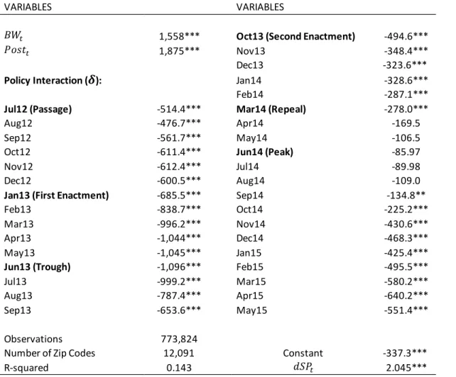
takes place this would indicate an immediate adjustment regardless of whether it was also anticipated. It is expected that the entire effect of BW12 was not anticipated and that there was some adjustment when the provisions took effect. However, the use of a moving average by Zillow may hide this structural break. It is also thought that the difference between areas will decrease when BW12 is repealed. Again, if this result is expected this may occur before March 2014. On the other hand, if the HFIAA is not seen as a significant improvement over BW12 the change in trend around this time may be minimal. When interpreting these results it is important to recall that correlation does not equal causation. No amount of correlation of the expected effects with the expected months can definitively show causation. The less they align the more doubt is cast on a causal relationship. Unless results are profoundly inconsistent with prior expectations or supremely aligned with them this model will always be open to interpretation. However, it provides as detailed look at the data at hand as is possible under the assumption that the model is well specified. Results are presented in Table 4.2. The coefficients on the treatment group time period interaction ( are displayed in Figure 4.1 along with their 95% confidence intervals. These coefficients represent the difference in the change in median home value growth between subsidized and non-subsidized areas; therefore, the difference from non-subsidized areas is represented by the x-axis.
Table 4.2: Difference in Changes in Median Home Values, Model III
VARIABLES VARIABLES
� 1,558*** Oct13 (Second Enactment) -494.6***
� 1,875*** Nov13 -348.4***
Dec13 -323.6***
Policy Interaction ( ): Jan14 -328.6***
Feb14 -287.1***
Jul12 (Passage) -514.4*** Mar14 (Repeal) -278.0***
Aug12 -476.7*** Apr14 -169.5
Sep12 -561.7*** May14 -106.5
Oct12 -611.4*** Jun14 (Peak) -85.97
Nov12 -612.4*** Jul14 -89.98
Dec12 -600.5*** Aug14 -109.0
Jan13 (First Enactment) -685.5*** Sep14 -134.8**
Feb13 -838.7*** Oct14 -225.2***
Mar13 -996.2*** Nov14 -430.6***
Apr13 -1,044*** Dec14 -468.3***
May13 -1,045*** Jan15 -425.4***
Jun13 (Trough) -1,096*** Feb15 -495.5***
Jul13 -999.2*** Mar15 -580.2***
Aug13 -787.4*** Apr15 -640.2***
Sep13 -653.6*** May15 -551.4***
Observations 773,824
Number of Zip Codes 12,091 Constant -337.3***
R-squared 0.143 � 2.045***
Robust standard errors *** p<0.01, ** p<0.05, * p<0.1
Note: The dependent variable is ∆ ��. Individual and monthly fixed effects are included but not reported.
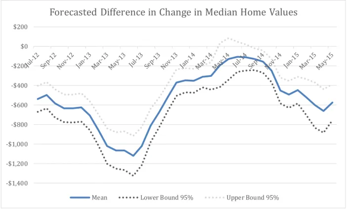
Figure 4.1: Forecasted Difference in Change in Median Home Values for Subsidized Areas, Model III
It is impossible to say for certain that BW12 is responsible for the difference in trends between areas with subsidies and without subsidies, but the evidence is compelling. The
difference in the change in monthly median home values peaks after BW12 is passed and occurs between the two enactment periods. This effect rapidly diminishes and become insignificant around the time BW12 is repealed. Oddly, it becomes significant again towards the end of the study period. It is also significant before BW12 is passed. It is still not clear that this correlation is not coincidence. Model IV extends this analysis into the past for a more complete picture of how home values correlate with NFIP reform over the course of the study. This model is given in Equation 4.4 and results are provided visually in Figure 4.2. Note the only difference from
Equation 4.3 is the extension of the summation back to = . -$1,400 -$1,200 -$1,000 -$800 -$600 -$400 -$200 $0 $200