Analysis of range with output linearly dependent upon storage, The

(1)

THE ANALYSIS OF

RANGE

WITH

OUTPUT

U

NEA

RLY DE

PE

NDEN

T

UPON STORAGE

By

Mirko

J. Mele

n

tijevich

Sept

embe

r

1965

(2)

THE ANALYSIS OF RANGE WITH OUTPUT LINEARLY DEPENDENT UPON STORAGE

September 1965

by

Mirko J. Melentijevich

HYDROLOGY PAPERS

COLORADO STATE UNIVERSITY

FORT COLLINS, COLORADO

(3)

ACKNOWLEDGMENTS

An expression of gratitude is given by the writer to those responsible for his support through a graduate research assistantship while at Colorado State University, to the

National Science Foundation for the support of the project through research grants, and to the National Center of Atmos

-pheric Research, Boulder, Colorado, for the use of its CDC

3600 digital computer system.

(4)

TABLE OF CONTENTS

Abstract

Mathematical Models 1. Introduction

2. Distribution function for cumulative sums, S., with output dependent upon those 3. Fokker-Planck partial differential equation fo\- cumulative sums, S . . . .

sums 4. The range of the cumulative sums, 5

i, with output dependent upon those sums II Testing and Improving Mathematical Models Using the Data Generation Method

1. Boundary conditions.

Z. Probability density function of cumulative sum. S

3. Properties of range. . . . . . . . . . . . . 4. Maximum surplus (Mn) and maximum deficit (m

n) of the cumulative sums, S 11l Distributions of Range, Surplus and Deficit as Obtained on the Digital Computer by the Data

Generation Method . . . .

IV Conclusions . . Bibliography Page ix I 2 3 4 7 7 8 9 14 19 28 29

(5)

Figures 1.1 2. I 2. 2 2.3 2.4 2.5 2.6 2. 7 2.8 2. 9 Z.IO Z. 11 Z. 1 Z Z. 13 2. 14 2. 15 2. 16

UST OF FIGURES AND TABLES

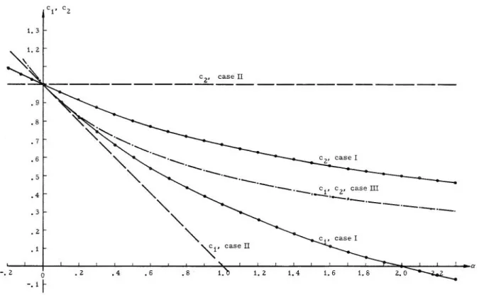
Constants c₁ and c₂ as function of a for three cases of boundary conditions.

Expression 1-e -20 t as function of a for various values of t . . .

Probability density functions, values of a . . . . • piS).

of the cumulative sum, S. at the time t. for various

The variance of cumulative sum S (-co < S < co) as a function of a and The mean range Rn as a function of n and a

for Var x " (Tz "

The mean range Rn as a function of n and a, for n. I - 12., as an enlargement of fig. 2.5 for small n

The variance of range, Var Rn as a function of n and a

The variance of range, Var Rn as a function of n and a for n = 1 - 12, as an enlarge-ment of fig. 2.7 for small n . . . . . . . .

The skewness coefficient of range, C

s (Rn) as a function of n and a

The kurtosis of range. Kr (Rn). as a function of n and a .

The mean ranges for n" 5, 10, 25 and 50, as a function of a.

Probability density functions, p(R), of range, for a O. 00, and a .. -0.020, and for n. 5, 10. 25 and 50 . . . . . .

Probability density functions, n'" 5. 10, 25 and 50 .

p(R), of range, for a" 0.100 and a 0.400 and for

Probability density functions, p(R), of range, for a" 2.000 and for n = 5, 10, 25 and 50

Correlation coefficients between Mn and mn for various values of a as a function of n

The ratio between Var [Rn] and Var [M

n], with Var [mnl .. Var [Mnl . . . .

2. 17 Skewness coefficients of maximum surplus (Mn) or maximum deficit (m

n) as a function of n and a

2. 18 The kurtosis of maximum surplus (Mn) or maximum deficit (m

n) as a function of n and a

2. 19 Discrete probability or probability mass tp (Mn) = 0 or p (m

n) 0] at zero values Mn" 0 or mn = 0, for -0.04

'5

a

'5

2.00 and 1 ~ n

'5

50

2.20 Probability density curves, p{M

n) or p{mn). for a = 0.00 and a " -0.020, and for

2. 21

2.21

n" 5, to, 25 and 50. The probability mass for Mn" 0 or fin"

°

is not shown on these graphS . .

Probability density curves, n" 5, la, 25 and 50. on these graphs . .

p(Mn) or p(mJ, for a" 0.100 and a" 0.400 and for The probability mass for Mn = 0 or m

n " a is not shown

Probability density curves, p (Mn) or p{m

n), for a:: 2.00 and for n" 5, 10, 25 and 50. The probability mass for Mn a or mn a is not shown on these graphs. . . .

vi 7 8 8 9 10 10 II IZ 12 13 13 14 14 15 15 16 16 17 18 18 19 19

(6)

Figures ,. I ,. Z

,

.

,

..

'

.

5 '

.

6

'. 7

'

.

8 ,

..

3.10 3. 11 3.1Z 3.13 3. 14 3. 15 3. 16 3.17 3.18 Tables ,. I ,. Z

UST OF FIGURES AND TABLES (Continued)

Distribution functions of range, FIR), for

_•

-0.040 and various values of n

Distribution functions of range, FIR), f.,

•

-0. OZO and various values of n

Distribution functions of range, FIR), fo,

_•

0.000 and various values of n.

_•

.. O. 100 and various values of n.

_•

O. ZOO and various values of n.

_•

• _•

Distribution functions of range, FIR), f. ,

••

Z.OO and various values of n

Distribution functions of maximum surplus, F(M

n), f., a • -0,040 and various values

of n

Distribution functions of maximum surplus, _F_(M_n_L fo,

• _•

-O.OZO and variOUS values

of n

n), f.,

•

.. 0.000 and variouS values

of n

Distribution functions of maximum surplus, F (M

n), f., a .. 0. 040 and various values

.f n

Distribution functions of maximum surplus, F(Mnl, fo, a-O. IOO and varIOUS values

.f n

Distribution functions of maximum surplus, F (MnL roc

..

o. ZOO and various values

.r n

Distribution functions of maximum surplus, F (MnL roc

• _•

0,400 and various values

.r n

n), roc

•

0.800 and various values

.r n

Distribution functions of maximum surplus. F(M

n), roc

•

Z.OOO and various values

.r n

Ratio of mean of range to standard deviation of the input, digital computer . . . • . • • . , . . . . .

(nn /.,.), obtained on the

Ratio of variance of range to the digital computer . . . .

variance of the input,

3.3 Correlation coefficient. p (M

n, mn), between the upper maximum sum, Mn' and the lower minimum sum, m

n. Page

"

Z3 Z3 Z3 Z4 Z4 Z4 Z5 Z5 Z5 Z6 Z6 Z6 Z7 Z7 Z7

zo

zt zt

(7)

ABSTRACT

The objectives of this investigation are twofold; (i) Deter -mination of the distribution function for the cumulative sums St when the output is dependent upon these sums; and (il) Development of probability expressions for the range of cumulative departures of a stochastic variable.

The basic relationship between input, output and cumulative sum is expressed by the equation of continuity

~

" qi (t)

-a

S; with

a

•

constant.

The following principal assumptions concern the fluctuating portion qi (t); (i) qi (t) is a normal independent variable with a mean of zero and a variance al_; _(ti) _The_correlation_{between the} values of qi (t) at different times tl and t

z exists only when

It 1 -

t21

is very small; (iii) qi (t) varies an extreme rapid amount when compared with the variation of the cumulative sum St.

Theoretical equations and hypothesis have been substantiated by the data generation method, which employs a digital computer. The large generated sample for computations consisted of 100.000 normal independent numbers, with mean zero and variance unity.

The large amount of data agreement between the data genera-tion method and that obtained from the theory indicates the validity of the theoretical equations.

The distribution function for the cumulative sums St when output is dependent upon those sums is defined by

The equations for the expected values and variance of range, R_n, are derived as (i+3aZ_e_-2a )

~

~ t=1 ix and -20 l H

(8)

THE ANALYSIS OF RANGE WITH OUTPUT UNEARLY DEPENDENT UPON STORAGE

By: Mirko J. Melentljevich

CHAPTER I

MATHEMATICAL MODELS

1. Introduction. Assume the availability of

a record (XkJ of mutually independent random varIa-bles with a common distribution f{x). The mean for these variables is assumed zero. Let Sn= XI

+

X

_z

+ ... + X and let

n

max min

The random variable

the cumulative sums,

random variable mn

cumulative sums. Si'

(0, 51' Sz,· ··, Sn] ,

{O, 51' Sz" , .• Sn]'

1.1

Mn is the maximum surplus of

5.

,

, with i '" 0, ... , n. The i& the maximum deficit of the

and the random variable

- m _n I.Z

is the range. These values are shown in fig. I. 1 where 0 1 is the time axis and 0 S the axis of the cumulative sums of mutually independent random variables with means zero. The curve representing

these sums is OABC, and OC is the time of n units.

5

,

Fig. 1. 1

,

'C

For the cumulative sums, 51' the maximum positive

sum DA is the maximum surplus, Mn; the maximum

negative sum EB is the maximum deli cit, mn: and

the sum DA + EB is the range, Rn' At present very few theoretical results are available for the charac-teristics of surplus, delicit and r~e. The results available are usually valid only for [X

k] normally distributed, with mean zero and variance cr1. Feller [4], in 1951, derived results for the asymptotic dis

-tribution of the range of the cumulative departures of a stochastic variable from its mean. In terms of the water storage-water yield relation in hydrology, his results apply to cases where the variable is the annual flow of a stream, with the annual draft equal to the mean annual flow, and a lengthy time period, In

particular, Feller obtained:

1. 60

Vn.

and

1.3 Var [Rn] " 0,2181 n

He assumed that (X

k] is a sequence of mutually ind e-pendent random variables with E [~J "0, and Var [Xkl • 1. Feller's asymptotic solution depends on the variance of Sn alone.

A. A. Anis and E. H. Uoyd (I, 1953] solved the planning storage capacity problem of a reservoir

when the water storage distribution over a given num -ber, n, of years is not known. The storage alter r years may be regarded as the sum of r annual incre

-ments. This real problem may be approximated by an ideal which has annual increments that are Ind

e-pendent variables with a common distribution.

Ap-plications to other storage problems are obvious. Anis and Uoyd derived the expected value of the range

over n years, as E [R _nJ - '

V;

If"

n-

I

E r= 1 1.4

In conclusion, they noted that the asymptotic value of the range for large n is

zFn

I. 5

which Is an agreement with Feller's results.

Thomas and Fiering [7] analyzed the follow -ing: (i) four record lengths (to, Z5, 50, and 100

years) for streamflow distributions (Normal, Gamma

with skewness -0.5, 0.5 and 1. 0); (ii) three serial correlation coefficients in annual flows (0. 0, O. 1 and 0.2); and (iii) three degrees of regulation (100 per-cent, 90 percent and 80 percent. Since the number of

parameter combinations increases in a multiplicative

rashion, 144 combinations defined the sample space for their Investigation. In each instance, the annual

nows are assumed to be derived from a population

with the mean unity and the standard deviation O. I5.

A digital computer was coded to generate a varied number of idential sets of data; for each combination they chose 100. The most important result of their study was the verification of HUrst's (5J and Feller's [4] theory with a constant outnow equaling the mean inflow. The agreement for small values of n is fairly close to Hurst's and Feller'S, and becomes ex·

tremely close as n increases. Computations based

on the formula given by Anis and Lloyd are only slightly better for n" 10 than those given by Hurst 'lnd Feller. The results of the study by Thomas and

(9)

Fiering indicate that the variance of the basic varia-ble is by far the most important parameter, even for relatively short record l~ngths. The relative unim-portance of skewness of the distribution of basic variables is clearly demonstrated. The serial cor

-relation tends to increase the required storage. This fact is also supported by the queueing theory.

2. Distribution function for cumulative sums, Sf' with output dependent upon those sums. The basic relation b~tween input, output and cumulative sum, Si' is expressed by the equation of continuity which for an incompressible medium may be written

..

1.6 where Q_i(t) is the input, Q

o (t) is the output, and dS/dt is the rate of change in time of the cumulative

sum 51" The symbol t relates here to a continuous

time series. When a discrete time series is used, the symbol n replaces t.

Here the input is taken as an independent stochastic variable, while the output is a dependent variable.

They are expressed here as:

Q

i (t) S Q

a .;. qi (t) I. 7

with Q_a• average input, and qi (1) nuctuating de

-viations ot input about Q a;

with Q

a " average output, and qo (t) fluctuating de -viations of output about Q

a. The basic proportionality of output to the cumulative sum, S, is

1.9

with 01 · constant, -co < a < co; and -co < 5 < co. Equations I. 7 through 1. 9 give the basic mathematical model tor the case studied in this paper as:

1. 10

Equation 1.10 is a Langevin equation for the Brownian motion of a free particle. As for the fluctuating part qj (t) the following principle assumptions are made for this equation: _. (1) The mean or q.

.

(t) is

zero, or

q;Ttr

s 0; (il) The correlation between the values of q. (t) at different times

t

,

and t2 exists only when

tt

l -

tJ is very small; (iii) qi (t) varies extremely rapidly compared to the variation of S; and (iv) qi (t) is normally distributed with mean zero and variance 1T2, The problem is to determine the

probability at which the cumulative sum, S, after the time t lies between Sand 5 + d 5, with S

=

So at

t .. 0 being the initial sum (or storage in the case of reservoirs).

,

The Langevin equation has been solved by many authors, using different integration methods. One solution of this equation was given by S. Chand

-rasekhar

[81.

His method of solution is used here to obtain a solution of eq. 1.

to.

Consequently, "solving" eq. 1. 10 should be understood in the sense of specifying a probability density distribution f(S, t; S). PhYSical

circum-o

stances or the problem require that f(S. t; S ) follow

o a distribution which is independent of So as

t-

-

"'"

1. 1 1 (2rIT0!)~

•

with IT S2 the variance of 5 for -00. This re -quirement on ((S, t; So) conversely requires that qi (t) satisfy certain statistical conditions. The general solution of eq. 1.10 is:

1. 12

Consequently. the statistical properties of

s - Soe-at 1.13

must be the same as those of

-

o

'J

' ,

e ea qi

m

d{.

1. 14 o

As t--4o(D, eq. I. 13 tends to S; hence the distribution

o

r

Lim ,~'"

must be the distribution

(Zr -s2/ZIT l

,

.

IT Z )~e

•

I. 15 1. 16

The right-hand side of eq. 1.

'2

may be written Cor e- .. jt.t as

I. 17

Le'

(10)

and the physical meaning of q (6t) is that it represents the input during an interval 6t. Equation 1. I Z then becomes

S - So e -u t •

7

eU (j6t - tl Q (6t) 1. 19

with the condition that the quantity on the rIght-hand aide tends to the distribution eQ. 1. 16 as I--..CD. This further requires that the probability of occur-rence of different values of q (6t) be governed by the distribution function

wl1ere

-

I

q

(6t)1 Z 12.6t fTZ

e I. ZO

.'

_•

.

I. 21

To prove this assertion the distribution function f(S, I; So) derived on the basis of eqs. I. 19 and 1. 20, does in fact tend to the distribution eq. 1. 16 as t -CD. Let

S 0

J

'..

!I)

q,

!I) d, .

o

1. 22

Then, the probability distribution of S is given by

t

-SZI2fTj61~

m

d~

,

f (S) • 1. 23

In order to prove this, the interval (0, t) is first divided into a large number or subintervals of dura-tion .e.t, so that

I. Z4

using eq. 1. t 9. S can be expressed in the form

S=1: \, 25

where

s;

•

6

1 (j.6t) q (At). I. Z6

According to eQ. I. 20, the probability distribution of

Sj is given as: Hence, f(S) [21f qZ 1: () 1 (j6t) 61)% e j t -SI/2qZ ~ 8 1l (j6t) J I. Z8 then. f(S) 0 t

~

6tZ(j.e.t).6t

",J6

_tZ₍₍₎_d_E' _. o which proves eqs. 1. ZZ and I. Z3. I. Z9 1. 30

The right-hand side of eq. 1. 12 may be expressed as

1. 31

with

8Im _eu(E -t) .

With the .foregoing definition of 8₁(E')' eQ. I. 30 governs the probability distribution of

I. 32

S - Soe-ut 1. 33

Since

1.34 and taking into account the relationship shown in eQ.

I.Zl then

f (S. t; So) :

-(5-5 e-utlZ/2(I_e-2ctt)fT Z

:-:--,----'0=;'--:0"';'

ir- '

0 ,

,[2" (I-e -lO't) "'s~] I

Therefore. eQ. I. 35 converges to

(2J"fT s Z _{/ ,} lor t-CD. _S1 /2q

,

~

,

I. 35 1. 36

This proves the assertion made that with the' statis -tical properties of q (lot) implied in eqs. 1. 20 and

1. 21. eq. 1. 19 leads to a distribution I (8. t; So) which tends to be independent of So as t_CD.

3. Fokker-Planck partial differential egua

-tion for cumulativ~ sums

a

S

,

The second method for deriving eq. 1.

35

is by a opting the Fokker-Planck partial differential ~quation lor cumulative sums, For this equation (8. t; So) is the fundamental solution.

When t increases by 61. 8 will in -crease by oS in the distribution function f (S, t; So),

(11)

Let the probability for an increase between the limits 65 and 65 + d (65) b~ f(65, 5, t) d (65), then

+ro

f(5+.65, t+ 6t; So) •

J

(5, t; So) (65, 5, t) d (t.S).

-00 1.37

Suppose that the probability of an increase,

as,

is In

-dependent of the fact that for t" 0, 5" So' then the integrand for powers of t.S is

r(5. t; So) f(65, 5, t) '" f{5 + 65, t) r (65, 5 + t.S, tl --<!oS (f' (5, t; So) f(65, 5, t) + + f (5, t; So) i' (.oS,S. t)] +

+ (is)!

[c"

(5, t; So) (68, 5, t) + + 2f1 (5, t; So) I' (65, 5, t) + +

r

(5) t; 50)!"

(~,

5,

t1+

'38

The resulting integrals all have simple meanings. For instance +ro fC(6S, 5+ t.S, t) d (t.S). I, 1. 39 -ro +ro

-J

65

r

(65, S, t) d (b.S) '" [65], 1. 40

J

:'

roo (.s, 5, e) d (.s).

a

Z _[_65Z]

a

(5+ 65)l 1. 41 -ro

and so on. Developing the left hand side in powers of 6t by using

r

,

(S+.s,

e),

)

!z (5 + bS, t); and assuming that

lim~

.e

.t--o .. 0;

then for 5 replacing 5

+

t.S

1

a

Zf(S,t;5) Z

r

2 (5, 1)---::--"'°

as'

Cor k > Z.

+

l

afZ(5~t)

_

as

1. 42 1. 43 4 ,1

a

f (5. I; 5) [, - f1 (5,1)1

as

0 ....

l'

arl(s,

I)]

-

as

l (5. t; 5). 1.44 The function f

t (5, t) and f2 (5, t) must be

deter-mined in order to verify the assumption of eq. 1. 43. It comes from the storage equation that

t + 61

lIS " - 0' 5 6t +

J

qi

m

ds. t. 45

e

As the mean of qi (E) is zero, then

[<!oS) • -0' 5.61" - 0' (5 + lIS) .6t, 1. 46 Which is obtained by neglecting the higher power terms of 6t. From this

lim

~

"

f (5+.65 t) .. - 0' (5 + lIS). 1.47

.6t ---.0 6t 1 •

In the same way, by neglecting the correlation be-tween the values qi (E) at E t and (2

1.48

so that:

f2 (5 + 65, t) " a-z • 20' fTsz = constant. 1.49

All the powers of 65 greater than one become pro -portional to like powers of 61, so that eq. 1.43 is satisfied. Therefore,

af (5, t; So)

at

which is the required Fokker-Planck partial differen -tial equation, of which eq. 1. 35 is then the fundamen -tal solution.

4. The range or the cumulative sums, Si'

with output dependent upon those sums. Let [q_{k J be} a sequence of mutually independent random variables with a common density function f(q), with E [qk

₁

·0

and Var [qk] " fTz. The basic eq. 1. 10 given in (fnite differences form

1. 51

(12)

Equation 1. 52: gives further for So " 0; So" 0; 52:. c ₂₊2 _a q2 + 2:(2: - a) (2: + a)Z ql ; 5, " ₂2 ₊_a q, + 2: ~2: - ai q, + 2: (2: - ail (2: + 0')1 ₍₂₊a)'

,

q, ; + 2:(2:-a) + (2: + 0')' qn-2: 2: (2: -

af

_q _-₃ ₊_{. . .} (2: + a) n where a is a constant. 1. 53

The maximum surplus of the cumulative sums, Si' for i " 0, t, ... , n is then, according to eq. 1. t, Mn" max [0, 51' 52:' ... , Sn

_l

and the maximum deficit is m

n" min [0, 51' 52:' ... , Sn1. The range is Rn" Mn - _{m n.}

The sums, Si' are asymptotically nor-mally distributed and, therefore, the asymptotic dis-tribution of the range is independent of the function

C(q). The sum Sn can then be considered as the value at time t" n of a continuously changing normal variable Se According to eq. 1. 35 with So· 0, 5

t is a normal variable with· mean zero and variance

.,.~ -2:a t

2:a (1 - e ). As t_oo, St approaches a

nor-mal va:·;.s.;;'le with mean zero and variance

.,.z

I

la. It

-2:0' t

should be noted that the term (1 - e ) is larger than 0.99 for t> 2:,303

Ill'.

(a) Mean and variance of range. The

mean range is E [Mn - mnl " E [Mnl - E [mnl.

Let Yn (x) be the probability density function of Mn and let .pn (x) and t - if; (x) be the distribution func

-tion, respectively, of Mn and m

n, so that

o

(x) · P (M < x) and 1/1 (x) • P

r (m~ ~ x). 1. 54

n r n - "

Let G_n(51' 52:' ... , Sn) be the joint distribution function of (51' 52:' . . . • Sn)' so that

and

corresponding to the observation that E [M 1 '"

-n E [mnl for symmetrical input distributions. The

function i:J

n (y) and 1/1 (-y) are thus integrals of the same type. If f (x) is an even function it follows that .pn (y) "lj; (-y).

For

a'"

0 it is very difficult to find

the exact analytical expression for the joint distribu-tion function G_n(51' 52:' ... ,Sn)' It is also practi

-cally impossible to derive general theoretical ex-pressions for the moments of range. If one accepts the hypothesis that the mean and the variance of range depend on the variance of St alone, for a given a, the following expressions are tested by the writer on a digital computer by the data generation method (Monte Carlo method):

and n

,

,. 1 n

,

I" 1 1. 57 I. 58 The constants C

l and C2: are functions of (l alone. Using the computer, for nine different values of a

(-0.04

'S

0"

'S

2:. 00). the expected values and variance of range were calculated for n between two and fifty. From these results it is found that the varia

-tions of C

1 "and C2: may be approximated by the

following expressions:

1. 59

>od

I. 60

Assuming that [qk

_J

is a normal variable with mean zero and variance unity, the following equations for the expected values and variance of range are ob-tained

and

(i+3aZ_e_-Za )

-V

a1f t.61

1. 62:

As a tends to zero, the expected values of ;:ange are the same as found by Anis and Uoyd (i} and the

vari-ance has the same form as derived by Feller [41, 1. e.,

-'If

0 1

E [R

J

"

-

E _-".=-;

n ... t-1 V t 1. 63

and

(13)

As a tends to infinity the expected values of range

and variance converge to zero,

(b) Correlation coefficient between Mn

and mn' The expreSSlon for the correlation coeffi-cient between Mn and mn is derived from the

general equation for the variance of Rn'

Var[R

n] • Var[Mn] + Var[mn] - l COY [Mn, mn} 1. 65 1. 67 Var [Rn]

l

var [Mn

_{l '}

1 - 1. 68 6

For n large. and a " 0, Var [R

1 "

0.l181n, eq.

2 n ~ ,r;c

1.31, and Var [Mnl " n(1-

if) -

lI' V n,

given by Anis [2]. For this case the correlation coefficient between Mn and mn becomes:

O. l181

P _{(Mn, mn)e l}- 2(1-2/l1') • 0.700. 1. 69

This value is verified by using the large amount of

random numbers simulated on a digital computer.

For a

I

0 the correlation coefficient between

M and m was obtained by using only random

n n

numbers and it was shown to be less than O. 700. If

a

- t

00 the correlation coefficient approaches

(14)

CH-I\PTER II

TESTING AND IMPROVING MATHEMATICAL MODELS

USING THE DATA GENERATION METHOD

1. Boundary conditions. Equations and hypo·

theses derived in the previous chapter have been pro·

ven by using the Monte Carlo or the data generation

method with Simulation of a large amount of random

numbers on a digital computer. The data used con·

sisted of 100, 000 random numbers of an independent

normal variable with mean zero and variance unity.

The program was such as to use random numbers in

blocks of 100, with a total of 1000 groups. The

cumu-lative sums of this variable are computed. The pro

-bability density distributions for the accumulated sum

during the period of n units, the accumulated sum at

the time n, the range, the upper maximum sum, and

the lower minimum sum, are obtained for the time

lags n ~ Z, 3, 4, 5, 6, 7, 8, 9, 10, lZ, 14, 16, 18,

ZO, 25, 30, 35, 40, 45 and 50. The first four mo·

ments are determined, both about the origin and

about the mean. The variance, the standard

devia-tion, the coefficient of variation, the Skew coefficient

and the excess are also computed for distributions of

each of the above statistics. All calculations were

made for the following nine values of the basic

para-meter Q': -0.040, -0.020, 0.000, 0.040, 0.100,

O. ZOO, 0.400, 0.800 and Z. 000.

The analysis of the problem with the

out-put being a linear function of the cumulative sums

shows different results depending on the boundary

conditions taken for the equation

c z' case Il

2. I

with c

t and Cz dependent on the following boundary

conditions.

Three cases for the integration of the

above equation are considered:

(1) Case 1. The instantaneous output de

-pends on the instantaneous value of cumulative sum,

S, with c₁ =(Z-0')/(Z+O'). andcZ=Z/{Z+a);

(Z) Case II. The output at the time n

depends on the value of cumulative sum, S. at the be

-.ginning of an interval, with c₁• 1 - 0", and

c

_z

"

I.DO; and

(3) Case III. The output at the time n

depends on the value of cumulative sum, S, at the end

of an interval, with

c

₁• C

z

= 1/(1 +0').

Only Case I produced the same results as

the theoretical examples derived in the previOUS

chap-ter.

Figure 2:.1 shows how the constants c_i

and C

z change with 0' for the three above cases.

The differences between these three cases increases

with an increase of 0' .

--- ---

---.9

.

· ,

.

,

· ,

..

.3

· ,

• >

-.

,

₀ -. >

~

Fig. Z. I

.

,

~'" " " , ... c_Z' case I

,

_,

.--

.--.--"

"

.-

.- ._ . c" c" cue 111 " -,-.!., ~ '\.

,

-'-

-

'

-

'

-

'

-

'

"'-" e ,casel '\.:' case II

.

,

.

,

.

>. > •• >.6 Constants c

(15)

-la t

The expression I - e which appears

in almost all equations of the previous chapter is

presente<" in fig. 2. 2. as a function of cr. for various

'.

0

· ,

.8

· ,

.6 .5

••

. 3

· z

•

values of t. with t " nil t and Il t " I, or a selected unit period. Therefore. t and n are

interchange-able in this text.

~---~--~--~---

--

---~

.

o

.1 .2 .l .4 .5 .6 .7 .8 .9 1.0

Fig. 2. l Expression I - e -lat as function of a for variOUS values of t

2. Probabilit densll function

or

cumulative sum. S. Probabi ity ensity unctlon 0 cumu at ve sum,

S,

at the time t" n l!. t. are shown in fig. 2. 3

for some particular cases. For the computation of

.

,.

,

.

,

₁_.._·o_.I_OO_._•_·._,._ooo_[

.

,

.

,--_

L..IIo\

----Re.ul .. from

eompu,or.

.'

.

these functions it was assumed that when t" 0,

So a 0, The computation was made by using eq. t. 35

for variOUS values of Q , and at different times t.

p ($) .·~.'OO:'·I ' 0,800: '? l - -.JII .•

..

,, ·O.~"O;'·'

.

,

.,

.

-

,

1 ... 0 .• 00." • 0 .• 00\

...·1.-Fig. 2. 3 Probability density functions, p(S), of the cumulative sum, S, at the time t. for various values of Q'

(16)

For a- " O. 100 and t" 3, the frequency density curve obtained by the computer is also given in fig. 2:.3.

These results are in agreement with the theoretical

results as obtained from eq. 1. 35. It can be seen from these graphs that for a- " O. 100 small differ -ences exist between the probability density curves for t " 8, and for t ~ 2:5. In fact, the process becomes

stationary for t::! 23. For a- " 0.400, the process

becomes stationary Cor t::: 6. The general conclusion is that the process becomes stationary for approxi

-mately

t:::

2:.3/(1. The probability density functions of cumulative sum, 5

n, accepted as being unchanged with time t for t ~, and they depend only on

a-for a given !T, or p(S

s

.

o)

..

L

....

~

n' a !T

V

'/r -a-5 llrrl I:: n -00

<

5

<

til l. l

'"

.

,

where uZ is the variance of input. For a normal in-dependent variable with mean zero and variance unity,

this equation becomes

p (S)

.,

~

n

V,

,

-0 5 l

n

Figure 2:. 4 shows the variance of the cumulative sum as a function of a- and 1. It can be

concluded that the variance decreases rapidly with an

increase of a-, and tends to become constant for a given a and

?

2:.3 a- glven y , b

l. 3

~---

--

---

.

o

.1 .~ .3 .4 .5 .6 .7 .8 .9 1.0

Fig. 2:.4 The variance of cumulative sum 5 (-00 < 5 < (0) as a function of a and t

for Var X" fJl " 1

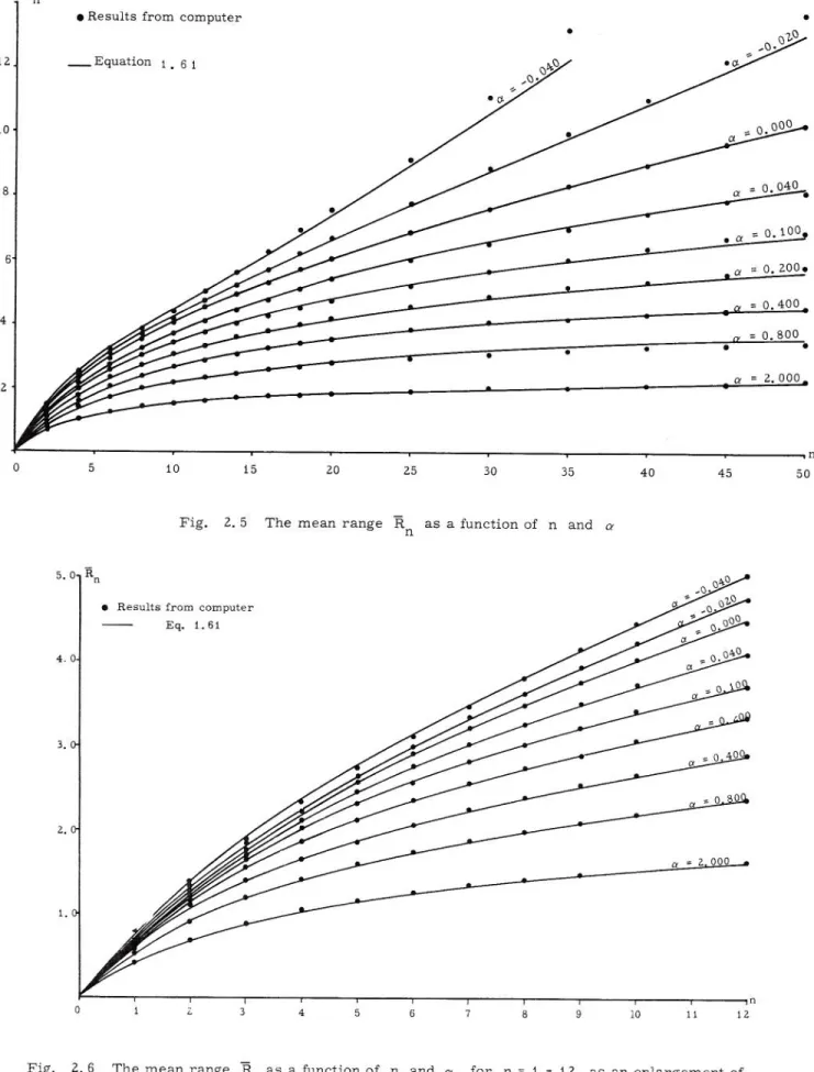
3. Properties of range. Figure 2:.5 shows the mean range for n values between zero and 50,

and a- " -0.04, -0.02:, 0.00, 0.04, 0.10, 0.2:0, 0.40, 0.80 and 2:.00. The points represent results obtained by the data generation method and the full lines re-present the values of eq. 1. 61. The hypothesis tested is that the basic shape of lines is defined by the

ex-pression LI

n (var S )~l

z:

t

t.l t 2.4

while the mean range is

2:. 5

The constant C

1 is a function only of a-.

This hypothesis is proved by the results obtained

from the computer. Using these results, the expres

-sion for the constant C

1 is determined and its values

are given by eq. 1. 59. It is nearly impossible to

cal-culate the exact values of mean range for a

I

0 even for n E 2:. Calculations obtained on the

compu-ter give the same results for the mean range as eq.

(17)

"

• ,

,

• Results from computer

• _",

,

'

.

•

_ Equation I. 6 1

",

.

,

"

.

• .

,

.. 0.000

,

.. 0.040 .. 0.10 0

•

0,200 • • 0

40'

. 0 800

•

2.000 ~--_ _ _ _ _ _ _ __ __ _ _ ~ _ __ _ _ __ ~ _ _ _ _ __ _ _ _ _ _ _ __ _ _ _ o

o

5

.

,.

,

.

Fig. Z.6 15 30 35

Fig. 2.5 The mean range

Rn

as a Cunction of n and a

• R",.ulu from computer

Eq. 1.61

The mean range

Rn

as a function of n and a . for

fig. Z,5 for small n

10

n • I - I Z, as an enlargement of

(18)

same moment. When n increases the number of

sub-samples of size n, as us cd on the computer,

de-creascs. Therefore, the abov~ differences may be the result of sampling errors. However, for any

practical purposes, these differences may be con

-sidered as negligible.

The mean range decreases rapidly with

an increase of /l, but the variance of output increases

with /l as

-Z/l t

Var Q = 0.5 a (1 - e ) .,.2.

o Z. 6 For a = 2.00 and sufficiently large values of t, and the variance of output is approximately equal to the variance of input,

.,.2.

For a < 0, the mean range and the vari-ance of output increases rapidly which is to be expect -ed when the cumulative sum, S, is larger than the

output is smaller or vice versa.

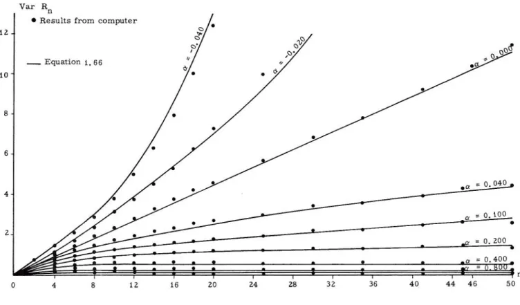
Var Rn

• Results Crom computer

IZ _ Equation 1. 66 10 8

_•

6 4

,

o

4 8 IZ 16

Figure Z. 7 shows the variance of range

for n between zero and 50, and the same 0' 's that

have been used for the computation of the mean range. The points represent the results obtained by the data

generation method and the lines represent eq. 1. 62. The hypothesis tested Is that the shape of lines is de

-fined by

Var 5

t

--,-

Z.7

The variance of range is

Z.8

The constant C

_z

is a function only of a. This

hypothesis is proved by the results obtained on the computer. The values determined for the constant

C

_z

are given by eq. 1. 60. The results obtained from

•

36

"

44 46 50

Fig, 2. 7 The variance of range, Var Rn as functions of n and a

the computer and the values of eq. 1. 66 coincide well

except for a smaller than zero. However, even for

a < 0 the differences are small. The variance of

range decreases faster than the mean range with a

identical increase of a. The skewness coefficients of

range for n between one and 50, and for various

values of 0' as obtained by the data generation method

are plotted in fig. 2. 9.

The kurtosis of range for various values of n and a as obtained by the data generation

(19)

5,0 Var R

"

4.0 3.0

'.0

o

• Results from computer

Eq. 1. 66

,

3 4

,

6 7

,

9 10

•

0 . 0. 100 • O. lOO Q -0.400 • • 0 - l 000

"

Fig. Z.8 The variance of range, Var Rn as a function of n and a , for n " 1 - I Z, as an

enlargement of fig. Z. 7 for small n

1.40 I. ZO p _OOOO 1.00 0.80 p ,. Q 949 0.60 ,. 0.400 0.40 ,, · 2.900 0.20

,

"

Z5

"

3S

Fig. Z. 9 The skewness coefficients of range, C

s (Rn) as a function of n and a

"

•

(20)

ot __ _{0 040} _0.020 0.00

---

0040

:::

_.:~

o 4 xv

,

.

,

0100 2.000

,

"

.,

~

'

L-

---",_

--

---;'~----

--

,~,,_

--

--_;.

,

;_----_;.~,,_--

--

"r,,;_----

_;

~---,,

--

,,---,:.-Fig. 2.10 The kurtosis of range, Kr(Rn) as a function of n and a

The mean ranges for n" 5, 10. 25 and 50 are shown in fig. 2. 11 as functions of a. It can

be concluded from these results that the mean ranges

decrease much slower with an increase of a from

"

up to about a • 0.4. The mean ranges decrease much slower with an increase of

a

from 0.4 to 1.0 than for a over 1. 00, where the decrease of the mean range with a is very slow.

n _ ~()

"

.

..

',,----1,f---.c,,---.:,

----

--.:

,---.:

,:----;,

-

.

;-

,

--

-;,-

.,;---:,-

.

;,----:

,-.~,----~

'

~.:---_;:l.

~

(21)

Probability density functions of range, for a few cases of n, for a given a are plotted in figs. 2. 1 Z, 2. 13 and 2. 14. Results are obtained on the computer. Feller [4J stressed that it is practically impossible to calculate the exact distribution of the range even for n" 3, with simple forms of a

distri-bution of inflows. From figs. Z. 1 Z, 2. t 3 and 2. 14,

..

·

,

.,

· ,

·

,

"

it can be concluded that with an increase of the para

-meter a the variance of the range decreases. The

computer results also show that for a >

°

and n > 51a the probability density functions for the

range are approximately normal with the means given

in fig. 2.5 and the variances given in fig. 2.7.

1 ~·O.ooo l

n • ~Q

"

_"

I

..

.

'0. oto

I

"

_"

Fig. 2.12 Probability density functions, p(R), of range, for a " O. ~O, and a = -0.020, and for n · 5, 10, 25 and 50 (R) ,

,

I

"

•

0.100

I

,

"

,; , ; N(7.0; Z.5) ,

,

.

,

R

o

4

,

"

0

Fig. 2. 13 Probability density functions, p (R), of range. for a

n" 5, 10, 26 and 50

14

1 ,,·0

.4

00

1

(22)

Fig. .8

.

,

.

.2 p(R)

· ,

•

· .

· ,

o·

~

o·

ir

n~Z5;50

<>~z

.

o

oo

l

\

~

UL~

__

~

____

__

____ --

R

,

_•

"

l. 14 Probability density functions, p(R), of range, lor 0' " l. 000 and lor n • 5,

to

Z5 and 50

---

~---4. Maximum surplus (Mnl and maximum

deficit (m l of the cumulative sums.

s

.

The mean

n

surplUS (Mnl or the mean maximum deficit (m_n) is

E [Mn

_l

'"

E [mnl • III E [R_{n l . As}fig. l.5 shows

the mean range, E [R

n]. as a function of nand 0',

half of the values of range of that graph represents

the means of surplus and deficit.

The correlation coefficients p

JM

n• mnl

between the upper maximum sum (Mn

_l

and the lower

minimum sum (m

n) for various values of n are

ob-tained by the data generation method and are plotted

in fig. l. 15. For Q '" 0, the correlation coefficient

Cor n-oo is calculated theoretically by using Feller's variance of range and Anis's variance of the upper maximum sum and lower minimum sum. The

same value is obtained on the computer. For a

I

0,

the correlation coefficients are obtained only on the

computer. For 0' ' O. the correlation coefficient

approaches O. 100 with an increase of n, and for

Q

I

0 it approaches zero.

Figure Z. 16 shows the ratio between the variance of range (Var Rn) and the variance of

maxi-mum surplus (Var Mnl or maximum deficit (Va.r m_n).

The varlancc of maximum surplus or maximum deli

-cit is defined by

2. 9

-Z(I-p[!"I1 • m

jj

.

n n

The skewness coefficients of maximum surplus (Mn) or maximum deficit (m

n) for n between t.",'o and 50 and for various values of a are plotted

in rig. l.11. For

0 OS

a ~ O.lOO the skewness

coef-ficients decrease with an increase of n. For a < 0

and a > O. lOO the skewness coefficients decrease

with an increase of n only for smail values of n, and

increase for large values of n. These results are

obtained on the computer by the data generation method.

a-O.OOO _ _ __ _ _ _ _ Q • 0.040

-

----

---

_0

-

-0. (1"2.0

-

---

_--

.

~ • 0 IOu

~

----===

~

q

-

o

.z

oo

a • 0 -100

..

<8

00

' L _ l 00 0

o

,

10

"

20 30

"

45 ;0

(23)

1.75 1.50 1.25 1.00 0.75 Vor (Rn) Vor (Mn) Q =2.000 0.400 0.200 0.10 _0040 ..().020 0.04 0.000 '0

"

'0

"

30

"

'0

"

.0 0 .. ~--

--

~

--

--~

--

~7-

--

~~--~

--

~--~

7---~~--~

----~

•

Fig. Z. 16 The ratio between Var [Rn

_l

and Var (Mn

_l

with (Var [mnl 5 Var [Mn

l

-• 0.000 • o. OiO " • ? 00 ~8 £9-_ - . 0400 • 0 20 • 0 I 0

!---

~

----

--",'

,

---c

,

'

,

----

---,

t

,

,---

-<

,

~

,

----

--c

,

"

,

---

,

.

,

--

----

-

.t,

,_----

-;

.,

r-

---,

,

>,

C"

0

Fig. Z.17 Skewness coefficients of maximum surplus (Mnl or maximum deficit (mnl as a function of n and a

(24)

Figure 2. 18 shows the kurtosis of maxi

-mum surplus (Mn) or maximum deficit (m

n) obtained on the computer by the data generation method. It

'0

.

,

'.0

"

' 0

clearly shows how the kurtosis changes as a func-tion of a and n.

a· -0.040

-0.020 __

-0.000

2o

L---

7-

₅

----~

₁₀

~----

~----~Cn----_,~----_t,,_

₁₅ ₂₀ ₂₅ ₃₀

----~--

₃₅

--_."'----_i

₄₀ ₄₅

c_--

--~~O

₅₀

Fig. 2. 18 The kurtosis of maximum surplus (Mn) or maximum deficit (m_n) as a function of nand Q

The discrete probability or probability

massior M .. 0 or m - 0 for 1< n < 50 is

n n

-shown in fig. 2. 19 as a function of a and n. It can

be concluded from these results that the probability

mass at Mn:= 0 (or m

n := 0) decreases rapidly with

an increase of both a and n. Results are obtained

on the computer by the data generation method. Some

probability density functions of Mn (or m_n) for

several values of n are plotted in figs. 2.20, 2.21

and 2. 22 for various values of a . It can be

con-cluded from these figures that the variance of the maximum surplus Mn decreases with an increase

of the parameter a . In fig. 2.21 for n. 50 and

a : O. lOa, it is shown that the probability density function of Mn is approximately normal with the mean 3. 50 and variance 2. 30. The probability mass

for Mn = 0 is not shown in figs. 2.20, 2. 21 and 2. 22. The probability density functions of Mn arc plotted in fig. 2. 20 as smooth curves. The smooth

curves were used to show the differences between

these curves and those developed for various values of n. Figures 2.21 and 2.22 show the curves as they came from the computer, obtained by the data generation method.

(25)

o. ,

0.'

Fig. Z.19

,.

,

.

,

_.

_,

Fig. 2. 20

"

• -0.040 • -O.OZO • 0.000 · 0 040 • 0, 100

•

Discrete probability or probability mass, p (Mn ., 0) or p (m

n • 0) at zero values, Mn 0 or mn 0, for -0,04 -: Q

'5

2.00, and

t

'5

n'5 50

"

...

"

,

"

.

.,

~::::::::~~~

"~

;;;;:;;:~~~==o====;.---

,,~:::

"

...

• 0 12 ,4 ••

Probability density curves, p (Mol or p (mnh for C1 ~ O. 00 and a· O. 020, and for n .. S, 10, 25 and 50. The nrobability mass for M O o r m 0 is not shown on these graphs

n n

(26)

,

. >

,

.1 .... 1 • • • 10 •• 1 ~. 0. 1001

.

·..,;.'u,

•• ,

.

"

.--"

---

'.

_.

_...

...

..

...

,J\

.t ... J . . . 1 ... 1

I •.

0 '00

I

1 v1

"1-"'''

J

~

.

"

\

\~

\\

~\..

'"

"''''''.

'

.

'

..

••

>.'

..

,>

Fig. 2.21 Probability density curves, p (Mn) or

p (m

n), for Q " O. 100 and a " 0.400

and for n · 5, 10, 25 and 50. The

pro-bability mass for Mn '" 0 or mn " 0 is not shown on these graphs

· I

_

.J

Of

.C

_.

J

..

'I

,

..

_1\

I

,

..

A\

)/i

\

I

r

l

~

,.> I I • . l,OOO '''0

,

.

H-.

.

"

/

1 I

~

"'''

'.0

\\

I

0.'

I

\

I

\

I

0.'

J

!

\

)

I

"

I

_\

Ii

"'

\

_\

\

/

I

0.'

.

~

)

1 ..

.

..

...

.> Q.

"

t.O t.4 t., u:

Fig. 2. 22 Probability density curves, p (Mnl or

p (m

n), for Q " Z. 000 and for n"' 5,

10, 25 and 50. The probability mass

for Mn" 0 or mn " 0 is not shown on

(27)

CHAPTER III

When the output Is a linear function of the cumulative sum it is useful to know the distributions of range, surplus and deficit for the normal independ -ent variable of the input. These distributions are

computed by the data generation method. employing a

CDC 3600 digital computer, from 100, 000 normal in -dependent random numbers. For different values of a the distributions are presented for the range and the surplus for various values of n. As the surplus is equal to the deficit, only the distributions of sur -plus are presented in this chapter.

The mean range Is given in table 3. 1 for n" 2:, 3, 4, 5, 6, 7, 8, 9, 10, 12, 14, 16, 18, 20,

25, 30, 35, 40, 45 and 50 for a - -0.04, -0.02:, O. 00,

0.04, 0. 10, 0.2:0, 0.40, 0.80 and 2.00.

The variance of range is given in table 3,2.

The correlation coefficient between the maximum

surplus (Mn) and the maximum deficit (m

n) are given In table 3. 3 for each of the above parameters of a and n.

From the data given in table 3. I, the mean

maximum surplus (Mn) and the mean maximum deficit

(m _n) can be computed by using the equation E [M _n

1

-E[m_n] - 112E [R

_n

]·

By using the data from tables 3. 2: and 3. 3, and eq. 2.9, the variance for maximum surplus (Mn) or

for maximum deficit (m

n) can be computed.

Distribution functions of range for a- -0. 040, and n . 2:, 4, 6, 8, 12:, 16, 20, 2:5 and 30 are plotted in fig. 3. I. Distribution functions of range Cor a '"

-0.02:0, 0.000, 0.040, O. laO, 0.2:00, 0.400, 0.800, and 2. 000, and for n · 2, 4, 6, 8, 12, 16, 2:0, 30,

40 and 50 are plotted in figs. 3.2: through 3.9. For some values of a and n, distribution functions of maximum surplus (Mn) or of maximum deficit (m ) are plotted in figs. 3.10 through 3. 18.

n TABLE 3,1

n/.

,

4 5 6 7 8

•

10

"

14 16 18 ZO Z5 30 35 40 45 50

Ratio of mean of range to standard deviation of the input, Rnl<r, obtained on the digital computer

-0.040 1. 402 1.894 2.327 2. 727 3.096 3.459 3.784 4.134 4.461 5.065 5.682 6.312 6.934 7. 595 9.2:69 I\. 152 13.372 15.784 19.000 23.402 -0.02:0 1. 382 1. 858 2:.271 2.650 2.995 3.328 3.623 3.931 4. 2:21 4.737 5.246 5.746 6.217 6.687 7.787 8.897 9.951 11. 042: 12. 2:67 13.636 0.000 I. 363 1.823 2. 2:21 2:.581 2.904 3.213 3.483 3.760 4. 022 4.477 4.917 5. 332 5.716 6.080 6.898 7.673 8.320 9.007 9.642: 10. 191 O. 040 1.325 1.760 2. 12:9 2.458 2.149 3. 02: 1 3. 2:57 3. 490 3.714 4.094 4.452 4.780 5.079 5. 348 5.949 6.513 6.947 7. 428 7.814 8. 145 0.100 1.274 1.678 2:.013 2.308 2. 566 2.802 3.009 3. 2:04 3. 398 3.719 4.025 4.2:92: 4.545 4.764 5.264 5.711 6.071 6.430 6.718 6.984

zo

0.200 1.200 1.564 1. 862 2.120 2:. 346 2:. 551 2:.733 2.898 3. 065 3. 340 3.606 3.824 4.032 4.205 4. 610 4.936 5. 2:18 5.457 5.648 5.834 0.400 1.082 1. 398 1. 654 1.876 2. 070 2:. 242 2. 397 2:.534 2.666 2.889 3. 096 3. 2:59 3.406 3. 52:3 3.807 4.018 4.204 4. ]48 4.477 4.589 0.800 0.92:3 I. 191 I. 410 1.595 I. 751 1.883 2.003 2. 103 2. 195 2. 354 2:. 489 2. 597 2.691 2:. 763 2. 945 3. 078 3. 195 3. 281 3.365 3. 435 2. 000 /).680 0.887 1.045 I. 168 1.267 I. 347 1.421 1. 478 I. 533 1.623 t.696 1.756 t. 808 .851 1.948 2.023 2:. 086 2:. 137 2. 183 2.22:1

(28)

TABLE 3.2

Ratio of variance or range to the variance of the input. cr~ [Rn 1Icr!, obtained on the digital computer

n/& -P. P-4P 2 0.648 0.923 4 I. 232 5 1.558 6 I. 912 7 2.370 8 2.683 9 3.2811 10 3.716 12 4.849 1-4 6. 194 16 7.767 18 9.935 20 12.359 25 20.291 30 32. -423 35 51.970 40 86.768 -45 134.872 50 211.738 -0.020 0.623 0.869

'"

1.404 t.687 2.040 2.2:;9 2.689 2.970 3.682 -4.439 5.269 6. Z80 7.331 10.001 13.496 17.5-49 24.183 .H.127 39.442 o. 000 O. 600 0.819 .050 1.273 I. SOl 1.777 I. 9H Z.247 2.439 2.910 3.360 3.817 4.320 4.812 5.790 6.982 7.798 9.-426 10.6ab 11.550 0.040 0.556 0.734 0.910 1.061 I. 22! 1.398 I. -485

'"

I. 766 Z.012 2.209 2.386 2.585 2.759 3.003 3.453 3.530 3.971 4.387 4.40-4 0.100 0.500 0.633 0.755 0.853 0.950 1.054 I. 106 I. 197 t. 256 t. 391 1.503 1.587 t. 715 1.807 1.931 Z.2Z0 2.260 2.438 2.631 2.540 TABLE 3.3 0.200 0.427 0.514 0.590 0.647 0.709 0.767 0.810 0.858 0.896 0.990 I. 060 I. 104 t. 1~9 I. 210 I. 257 I. H2 I.H6 I. 417 I. 417 1.356 O. -400 0.331 0.382 O. -429 O. -'164 0.506 0.536 0.567 0.588 0.607 0.645 0.664 0.671 0.681 0.682 0.675 0.668 0.655 0.675 0.635 0.620 0.800 0.235 0.275 0.30B 0.327 0.346 0.349 0.358 0.360 0.357 0.357 0.350 0.344 0.338 0.334 0.320 0.30-4 0.296 0.298 0.280 0.267

Correlation coefficient, p (M

n, mn). between the upper maximum sum, Mn, and the lower minimum sum, mn nla -0.040

• ,

,

8 9

"

..

\6

"

ZO 25 3D 35 40 <5 50 0.567 0.605 0.621 0.633 0.633 0.635 0.645 0.640 1).6-40 0.6-40 0.635 0.635 0.632 0.617 0.503 0.588 0.573 0.536 0.522 0.522 -0.020 0.570 0.507 0.626 0.636 0.641 0.654 0.650 0.654 0.656 0.657 0.656 0.655 0.654 0.662 0.546 0.646 0.646 0.620 0.610 0.614 0.01)0 0.570 0.615 0.636 0.6-42 0.648 0.650 0.664 0.660 0.665 0.662 0.670 0.670 0.672 O. 674 0.682 0.680 0.694 0.678 0.675 0.692 I). 0-41) 0.575 0.612 0.634 0.646 0.654 0.657 0.667 0.669 0.670 0.670 0.673 0.576 0.575 0.678 0.680 0.665 0.662 0.648 0.622 0.635 0.100 0.575 0.616 0.635 0.650 0.657 0.658 0.662 0.666 0.664

o

654 0.648 0.641 0.630 0.632 0.605 0.550 0.548 0.500 0.455 0.455 0.200 0.615 0.614 0.630 0.640 0.640 0.640 0.630 0.627 0.614 0.586 0.560 0.544 0.518 0.500 0.450 0.400 0.375 0.320 0.300 0.300 O. 400 0.568 0.595 0.596 0.580 0.570 0.553 0.526 0.511 O. -494 0.4-46 0.410 0.380 0.360 0.342 0.285 0.260 0.235 O. 181 O. 190 O. 185 0.800 0.528 0.51S 0.480 O. -450 0.410 0.392 0.356 0.335 0.315 0.272 0.2-47 0.222 0.207 0.200 0.156 O. 146 O. 134 0.096 O. 100 O. 108 2. POP

o.

j 48 0.172 O. 179 O. 177 O. 173 O. 168 O. 163 0. 161) O. 153 O. 1-46 O. 1-40 O. 133 0.131 O. 128 O. 121 O. 114 0.107 O. IP5 O. 101 0.096 2.000 0.330 0.250

o.

195

o.

160 O. 135

o.

118 0.095

o

080 0.080 0.060 0.040 0.040 0.035 0.025 0.005 0.020 0.030 0.020 0.020 0.040

(29)

F(R)

1.00

I

(1'-0.040

Fig. 3. I Distribution functions of range, F (R), for a '" -0.040 and for various values of n

F (R)

"

<I' --0.0201

,

,V~~~~~~~~

- 6 8

--

~--~--~--7.c--7.0--~~~~~~

10 12 I_ 16 18 20 22 24 Fig. 3. Z Distribution functions of range, F (R), for a" -U. UlO and various values of n

F (R)

"

(I. 0 000

,

"

_"

Fig. 3. 3 Distribution functions of range, F (R). for a" 0.000 and various values of n

(30)

f (R)

0.'

.. . 0.0"10

o.

0.'

Fig. 3,4 Distribution functions of range, F (R), for a 0.040 a.nd various values of n

F (R) '0 0.' 0.' a • 0 100 0.' 0 '

Fig. 3.5 Distribution functions of range, F (R), for a 0.100 and various values of n

f (R I

o.

0.' a • 0 200

o

·

0.'

(31)

F IRI

,

.

••

a • 0.400

.

,

..

.

,

.

V~~~~

-

~

3

--7---7---

4 '

7. ---7

--

-7---7--

a 9

~~

10

~

11

~~

12

~-Fig. 3. 7 Distribution functions of range, F (R). for 0' D. 400 and various values of n

F Iltl

••

0.' ..• 0.100

• .

.

,

.

,.

'.0

.

•

'.0

"

..

Fig. 3.8 Distribution functions of range, F (R). for a D, 800 and various values of n

FIR)

" • 2.00

o

Fig. 3.9 Distribution functions of range, F (R), for a " Z. 00 and various values of n

(32)

F(hlnlor F(mn) "

,

.•

Fig. 3. 10 a ' -0.040

,

_•

"

_"

n), for a -0.040 and various values of n F ( hln) " Fig. 3. t 1

,.

,

Fig. 3.12 a ' -0.020

,

_•

,

_•

"

n), for a -0.020 and various values of n

• • 0.000

,

_•

,

_•

"

Distribution functions of maximum surplus, F (Mnl. for a 0.00 and various values of n

"

.,

(33)

F ''''II) " 11.' 0.040

••

Fig. 3.13

•

• ,

•

• _"

_"

n), for a 0.040 and various values of n F ("'n J "

,

.

,

.

,

.

•

Fig. 3, 14

•

• ,

.

,

,.

• .'

.'

.

,

a • 0.100

"

,.

..,

.

,

•

• ••

•

n), for- a 0,100 and various values of n F (~n )

,

.

,,'

• ,

.

II • O.lOO

,

.

..

.'

..

,

.

"

.

•

• ••

.

,

•

• .

.

,

•

Fig. 3. 15 Distr-ibution functions of maximum sur-plus. F (M ), for- a .: 0.200 and var-ious

values of n n

(34)

f (M"l Fig. 3.16

,

.

•

Fig. 3.17 fIM,,) Fig. 3. 18 • • 0 .• 00

••

Distribution functions of maximum surplus, F (Mn), [or cr ~ 0.400 and various values of n

•

• ,

.

,

.

_•

,

.

n), for a • 0.800 and various values of n

• • l . 0 0

••

,

.

,

.

Distribution functions of maximum surplus, F (Mn), for cr . Z. 00 and various values of n

(35)

CHAPTER V CONCLUSIONS

The following conclusions are based on the analysis of the range when the output is linearly de -pendent on the cumulative sum:

(I) For a

I

0, it Is practically impossible to derive a general theoretical expression for the

range distributions or their moments even for very small values of n, such as Z or 3.

(2) The agreement between results obtained by the data generation method on a digital computer and the theory derived in this study. indicates that the hypotheses tested in the development of theory are confirmed.

(3) Probability density functions of the

cumu-lative sum at the time t become approximately sta

-tionary (or t ? 2. 3/01.

(4) Equations t. 61 and 1. 62 gives the mean

range and the variance of range. respectively. They are derived under the hypothesis that the mean range and the variance of range depend only on the variance of the cumulative sum at the time t for a given 01.

As 01 tends to zero the mean range tends to the same expression as it is found by Aois and Lloyd and the variance tends to the same expression as derived by Feller.

28

(5) The probability density function for the

range for t > 5/01 is approximately normal. with the mean as shown in fig. 2.5 and the variance as Shown in fig. 2.7.

(6) The general expression for the correla_ tion coefficients between the maximum surplus (l\rt )

n

and the maximum deficit (m

n) of the cumulative surns

is related to the variance of Rn' but the values

ot

these correlation coefficients are obtained on a digital computer by the data generation method.

(7) The mean range and the variance of

range decrease rapidly with an increase of a, While the variance of the output increases with an increase of 01.

(8) The variance of the basic input variable is by Car the most important parameter which affects the characteristics of range. surplus and deficit fOr

(36)

BIBLIOGRAPHY

L Anis, A. A., and Uoyd, E. H., On the range of

paMial sums of a finite number of independent

normal variates. Biometrika, Vol. 40; pp. 35 -42, 1953.

2. Anis, A. A., The variance of the maximum of

partial sums of a finite number of independent

normal variates. Biometrika, Vol 42; pp. 96-101, 1955.

3. Arns, A. A., On the moments of the maximum

of paMial sums of a finite number of independent

normal variates. Biometrika, Vol. 43; pp. 7

9-84, 1956.

4. Feller, W., The asymptotic distributions of the range of sums of independent random variables.

Annals of Mathematical Statistics, Vol. 2l; pp.

427-432, 195 ..

5. Hurst, H. E., Long term storage capacity of re -servoirs. Transactions of the American Society of Civil Engineers, Vol. 116; pp. 770-808, 1951. 6. Melentijevich, M. J., Characteristics of storage

when outflow is dependent upon reservoir volume. Ph. D. Dissertation, Colorado State University,

1965, 96 p.

7. Thomas, A. H., Operation research in water

quality management. Harvard University Div

i-sion of Engineering and Applied Physics, Chap-ter I; pp. l - l6, 1963.

8. Wax, N., Selected papers on noise and stochastic

processes. New York, Dover Publications, 1954.