Wellbore stability analysis based on a new true-triaxial failure criterion

(1)

TRITA-LWR PHD 1026 ISSN 1650-8602

ISRN KTH/LWR/PHD 1026-SE ISBN 91-7178-406-3

W

ELLBORE

S

TABILITY

A

NALYSIS

B

ASED ON A

N

EW

T

RUE

-T

RIAXIAL

F

AILURE

C

RITERION

Adel Al-Ajmi

(2)

(3)

Wellbore stability analysis based on a new true-triaxial failure criterion

i

Abstract

A main aspect of wellbore stability analysis is the selection of an appropriate rock failure criterion. The most commonly used criterion for brittle failure of rocks is the Mohr-Coulomb criterion. This criterion involves only the maximum and minimum principal stresses, σ1 and σ3, and therefore assumes that the intermediate stress σ2 has no influence on rock strength.

When the Mohr-Coulomb criterion had been developed, it was justified by experimental evidence from conventional triaxial tests (σ1 > σ2 = σ3). Based on triaxial failure mechanics,

the Mohr-Coulomb criterion has been extensively used to represent rock failure under the polyaxial stress state (σ1 > σ2 > σ3).

In contrast to the predictions of Mohr-Coulomb criterion, much evidence has been accumulating to suggest that σ2 does indeed have a strengthening effect. In this research, I

have shown that Mohr-Coulomb failure criterion only represents the triaxial stress state (σ2 = σ3 or σ2 = σ1), which is a special case that will only occasionally be encountered in situ.

Accordingly, I then developed a new true-triaxial failure criterion called the Mogi-Coulomb criterion. This failure criterion is a linear failure envelope in the Mogi domain (τoct-σm,2 space) which can be directly related to the Coulomb strength parameters, cohesion and friction angle. This linear failure criterion has been justified by experimental evidence from triaxial tests as well as polyaxial tests. It is a natural extension of the classical Coulomb criterion into three dimensions.

As the Mohr-Coulomb criterion only represents rock failure under triaxial stress states, it is expected to be too conservative in predicting wellbore instability. To overcome this problem, I have developed a new 3D analytical model to estimate the mud pressure required to avoid shear failure at the wall of vertical, horizontal and deviated boreholes. This has been achieved by using linear elasticity theory to calculate the stresses, and the fully-polyaxial Mogi-Coulomb criterion to predict failure. The solution is achieved in closed-form for vertical wellbores, for all stress regimes. For deviated or horizontal wellbores, Mathcad programs have been written to evaluate the solution. These solutions have been applied to several field cases available in the literature, and the new model in each case seems to be consistent with the field experience.

Keywords: failure criteria, Mogi failure criterion, intermediate principal stress, polyaxial test data, wellbore stability.

(4)

(5)

iii

Acknowledgments

I wish to thank everyone who added to the value of the work described in this thesis and to the pleasure I gained from it. I would like to express my deepest thanks and gratitude to Professor Robert Zimmerman for being an outstanding advisor and excellent professor. His constant encouragement, support and invaluable suggestions made this work successful. Robert, I was so lucky being your student.

I acknowledge and thank Sultan Qaboos University of Oman for their sponsorship and continuous support.

I am grateful to my colleagues in Petroleum Engineering and Rock Mechanics Group at Imperial College of UK for their comments and cooperation during my PhD studies in London. In particular, I would like to thank Mohammed Al-Gharbi for his fruitful discussions and especially encouragement. I would like to extend my gratitude to Dr. John Harrison for allowing me to participate in teaching rock mechanics and engineering for various bachelor and master degree programs in Imperial College. I would like to thank Yahya Al-Wahaibi, Sultan Al-Mahrooqi, Mohsen Masihi, Hassan Mahani, and Abdolnabi Hashemi for discussions and friendship.

A special thanks goes to Talal Al-Wahaibi, my colleague in Sultan Qaboos University, for cooperation and friendship during my research. Abduljalil Moosa, the cultural attaché at the embassy of Sultanate of Oman in London is acknowledged for his support and cooperation. I am grateful to my colleagues in the Engineering Geology and Geophysics group at KTH for all the discussions and cooperation. I would like to express my gratitude to Dr. Joanne Fernlund, and Dr. Lanru Jing for their cooperation and providing a good working atmosphere during my study in Stockholm. The friendship of Alireza Baghbanan, Thushan Ekneligoda, Tomofumi Koyama and Ki-Bok Min is much appreciated. My thanks also go to Britt Chow for effective and kind help with all administrative work.

Last, but not least, I would like to thank my wife, Um-Ammar, for her understanding and love during the past few years. Her support and encouragement was in the end what made this dissertation possible.

(6)

(7)

v

Some of the work contained in this dissertation is also contained in the following papers:

1. Relation between the Mogi and the Coulomb failure criteria, A. M. Al-Ajmi and R. W. Zimmerman, Int. J. Rock Mech., vol. 42, pp. 431-39, 2005.

2. Wellbore stability analysis using the Mogi-Coulomb failure criterion, A. M. Al-Ajmi and R. W. Zimmerman, in 40th U. S. Symp. Rock Mech., Anchorage, Alaska, paper ARMA 05-784, 25-29 June 2005.

3. Stability analysis of vertical boreholes using the Mogi-Coulomb failure criterion, A. M. Al-Ajmi and R. W. Zimmerman, Int. J. Rock Mech. (in press, as of 1 May 2006).

4. A new 3D stability model for the design of non-vertical wellbores, A. M. Al-Ajmi and R. W. Zimmerman, in 41st U. S. Symp. Rock Mech., Golden, Colorado, paper ARMA 06-961, 26-30 June 2006.

5. Stability analysis of deviated boreholes using the Mogi-Coulomb failure criterion, with applications to some North Sea and Indonesian reservoirs, A. M. Al-Ajmi and R. W. Zimmerman, SPE Asia-Pacific Drilling Technology Conference, Bangkok, Thailand, 13-15 November 2006.

(8)

(9)

vii

1

Introduction

Oil fields are usually drained from several platforms that extensively influence the development costs. The required number of platforms can be reduced by using non-vertical production wells. The deviated and horizontal wells will enlarge the drainage area from a single point. This will increase the productivity, and may subsequently decrease the number of planned platforms. In some cases, deviated boreholes are drilled to reach a substantial distance horizontally away from the drilling location (i.e., extended reach drilling). This is mainly used to access many parts of the reservoir from one location, which will also reduce the required number of platforms. Moreover, deviated boreholes are some times essential to reach locations that are not accessible through vertical boreholes. However, drilling non-vertical boreholes brings out new problems, such as cuttings transport, casing setting and cementing, and drill string friction. An increased borehole angle will also increase the potential for borehole instability during drilling. Therefore, a substantial savings in expenditure can be achieved if non-vertical wells can be drilled, while avoiding instability problems during drilling.

Nevertheless, drilling vertical boreholes will not guarantee the stability of the well. In all areas of the world, borehole instability causes substantial problems, even in vertical boreholes. For instance, in the Wanaea field of the Australian Northwest Shelf, the development plan proposed deviated and horizontal wells to minimize stability problems (Kingsborough et al., 1991).

Wellbore stability is dominated by the in situ stress system. When a well is drilled, the rock surrounding the hole must take the load that was previously taken by the removed rock. As a result, the in situ stresses are significantly modified near the borehole wall. This is presented by a production of an increase in stress around the wall of the hole, that is, a stress concentration. The stress concentration can lead to rock failure of the borehole wall, depending up on the existing rock strength. The basic problem is to know, and to be able to predict, the reaction of the rock to the altered mechanical loading. This is a classical, though not very easy, rock mechanics problem.

In order to avoid borehole failure, drilling engineers should adjust the stress concentration properly through altering the applied internal wellbore pressure (i.e., mud pressure) and the orientation of the borehole with respect to the in situ stresses. In general, the possible alteration of the borehole orientation is limited. It is therefore obvious that wellbore instability could be prevented by mainly adjusting the mud pressure. Traditionally, the mud pressure is designed to inhibit flow of the pore fluid into the well, regardless of the rock strength and the field stresses. In practice, the minimum safe overbalance pressure (well pressure − pore pressure) of typically 100-200 psi, or a mud density of 0.3 to 0.5 lb/gal over the formation pore pressure, is maintained (e.g., French and McLean, 1992; Awal et al., 2001). This may represent no problem in competent rocks, but could result in mechanical instability in weak rocks. In general, the mud pressure required to support the borehole wall

(12)

is greater than that required to balance and contain fluids, due to the in situ stresses which are greater than the formation pressure.

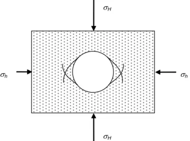
Stress-induced borehole failures can be grouped into the following three classes, as shown in Figure 1.1:

• Hole enlargement or collapse due to brittle rock failure of the wall. Symptoms of this condition are poor cementing, difficulties with logging response and log interpretation, and poor directional control. Poor cementing of the casing could lead to problems for perforating, sand control, production and stimulation. Furthermore, when the hole starts to collapse, small pieces of the formation may settle around the drill string and pack off the annulus (i.e., hole pack-off), while medium to large pieces fall into the borehole and might jam the drill string (i.e., hole bridging). These may prevent pulling the string out of the hole (i.e., stuck pipe), and so the planned operations are suspended. Stuck pipe problems due to borehole collapse is illustrated in Figure 1.2.

• Hole size reduction due to ductile rock failure presented by the plastic flow of rock into the borehole. This usually occurs in very weak shale, sandstone, salt and some chalk formations. Symptoms of this condition are repeated requirements of reaming and may result in stuck pipe.

• Tensile splitting of the rock from excessive wellbore pressures (i.e., hydraulic fracturing). Severe loss of drilling fluid to the formation from fracturing often causes well control problems. The lost circulation will reduce the applied mud pressure and may result in inflow of pore fluid. The formation fluid will flow from high pressure zone (kick zone) to a lower pressured zone (loss zone), which is known as under ground blowouts

Unplanned operations due to stress induced borehole failure resulting in loss of time and occasionally equipment account for at least 10% of drilling costs (Ewy et al., 1994; Santarelli et al., 1996; Aadnoy and Ong, 2003). For instance, Charlez and Onaisi (1998) presented two examples of stuck pipes due to wellbore instability in the Dunbar field (northern part of the North Sea). In both examples sidetracking of the well was essential and the cost was in the range of $2M for each case.

1.1 Other parameters affects borehole stability

We have highlighted that borehole instability is governed by in situ stresses, pore pressure and rock strength. In addition to these dominant parameters, borehole stability may directly or indirectly be influenced by the following parameters or effects: (a) mud chemistry, (b) temperature effects and (c) time-dependent effects.

Most of the overburden consists of shaly formations. In highly reactive shale sections, mud chemistry is of extreme importance in addition to the mechanical aspects of instability. The mud composition changes as shales slough and disperse into the mud column, or by chemical interactions between the minerals in the formation and the mud. This indeed will alter the mud properties and rheology. Therefore, chemical additives are typically introduced in the mud according to the minerals in the formations. In highly reactive shales, oil-based mud is preferred as it is more inhibitive than water based mud. However, the disposal of oil-based

(13)

Introduction

3

mud requires a special management to avoid the pollution of the environment, which has restricted its applications.

(a) (b)

Figure 1.2. Stuck pipe problem due to borehole collapse. (a) Hole pack-off. (b) Hole bridge.

(14)

Temperature changes associated with mud circulation during drilling may alter the rock properties (Fjaer et al., 1992, p. 254). The change in rock properties may reduce or enhance borehole failure depending on the thermal effect. Maury and Sauzay (1987) reported that temperature fluctuations may also influence the stress distribution around the borehole. As the temperature increases, the tangential and vertical stresses will increase. However, temperature fluctuations will not influence the stress anisotropy around the borehole as the thermal effect should alter the tangential and vertical stresses by an equal amount (Zhou et al., 1996).

Reactive shale instability is also time-dependent, and is governed by two intrinsic mechanisms: (a) consolidation and (b) creep. Consolidation is due to pore pressure gradients induced by fluid communication between the mud and pore fluid. Creep is described by a change of strain at a constant effective stress level. Both of these mechanisms will result in hole size reduction. In practice, it is difficult to distinguish between creep and consolidation effects. In general, consolidation will occur shortly after loading, while creep will govern later deformation (Fjaer et al., 1992, p. 253). The mud pressure and properties, and the temperature in the rock may vary during drilling operations, which in turn enhance borehole instability. All these parameters make it more difficult to directly pursue the time-dependent effects. The best approach is to quickly isolate the rock with a casing to minimize the potential borehole instability.

1.2 Motivation for studying wellbore stability analysis

Wellbore stability problems in exploration and production drilling cost the drilling industry certainly more than $100 million per year worldwide, and may approach one billion dollars annually. “Despite tremendous efforts pursued over the past years, wellbore stability problems continue to be experienced by the drilling communities. The practical consequences of wellbore instability are often the collapse of borehole wall” (Aadnoy and Ong, 2003). Borehole collapse could be predicted by adopting compressive failure analysis in conjunction with a constitutive model for the stresses around the borehole. The selection of a failure criterion for wellbore stability analysis is difficult and confusing (see, for example, McLean and Addis, 1990a). It is unclear to drilling engineers as which failure criterion should be used in the wellbore stability analysis.

“Preferably a failure criterion should be based upon knowledge of the failure mechanism, but this is not always so. In fact, many failure hypotheses have been propounded as a result of theoretical reasoning only and could not be verified by experimental evidence” (Bieniawski, 1967). The most commonly used failure criteria in wellbore stability analysis are Mohr-Coulomb criterion and Drucker-Prager criterion. These failure criteria are based on quite different failure hypotheses. The Drucker-Prager criterion considers the influence of all three principal stresses on failure, while the Mohr-Coulomb criterion implicitly ignores the influence of the intermediate principal stress on failure. Despite this difference, both of these failure criteria have been verified experimentally to be good in modelling rock failure, based on conventional triaxial tests (σ1 > σ2 = σ3). On the other hand, in practice, the

Mohr-Coulomb criterion has been reported to be very conservative in predicting wellbore instability, while the Drucker-Prager criterion has been found to be overly optimistic about wellbore stability.

In the field, the wellbore is normally under a polyaxial stress state (σ1 >σ2 > σ3), and the

conventional triaxial stress state is a special case that may only occasionally be encountered in situ. Neither the Mohr-Coulomb criterion nor the Drucker-Prager criterion are based on

(15)

Introduction

5

polyaxial failure mechanics. Actually, these failure criteria have been developed prior to the construction of the first apparatus that enabled true-triaxial tests. Hence, it is not surprising that these failure criteria are not very good in modelling borehole failure.

This research will study the basic fundamentals of stress and rock failure mechanics. In this work, we will examine if the failure criteria can really be verified experimentally, based on polyaxial test data rather than triaxial test data, which is more appropriate to field scenarios. The main objectives of the research are to choose and, if necessary, develop the most suitable failure criterion in representing polyaxial failure mechanics. This true-triaxial failure criterion will be then utilized to develop a new three-dimensional stability model to prevent vertical, horizontal and deviated borehole failure. The subject of borehole failure is quite complex and confusing. For simplicity, therefore, we will only consider the mechanical instability of the wellbore in this research. The ultimate objective of the research is to improve borehole failure predictions, in order to minimize wellbore stability problems experienced by the drilling communities.

(16)

(17)

Basic theory of stress

7

2

Basic theory of stress

The concept of stress and its analysis in a generally loaded solid is not trivial, yet it is thoroughly fundamental for all work on rock mechanics. Stress inside a body will in general be non-uniformly distributed. It is not just a single value (i.e., a scalar), but a tensor quantity which has six independent components that will act and be sustained at any point inside the body. The evaluation of stress components is a matter of pure statics. These and other relevant concepts are elaborate in the following sections.

2.1 Stress at a point

If a body is uniformly loaded, stress can be thought of simply as force divided by the area of application. For instance, if a cylindrical homogenous solid having cross-sectional area A is compressed vertically by a uniformly distributed force F as shown in Figure 2.1(a), the vertical stress σ acting on and inside the cylinder is defined as

. F A

σ = (2.1)

In rock mechanics, stress is frequently measured in N/m2_{, that is, Pa (Pascals). Other units}

encountered include psi = 6.895 kPa, kg/cm2 = 98.1 kPa, and bar = 100 kPa. Furthermore, positive stresses are considered to be compressive and negative stresses are considered to be tensile. This is opposite to the sign convention used in other sciences involving elasticity.

Figure 2.1. Definition of stress.

The stress is always associated with a particular cutting plane. To illustrate this, consider the cross section A′ in Figure 2.1(b). Here the area A′ is greater than A, and the force is no longer normal to the cross section. The force can be decomposed into one component Fn that is

F F A F F A’’ A (b) (a)

(18)

normal to the cross section, and one component Fs that is parallel to the section (Figure 2.2). The quantity n n F A σ = _′ (2.2)

is called the normal stress, whereas the quantity

s F A

τ = _′ (2.3)

is called the shear stress.

Therefore, the area of the cross section and its orientation relative to the force are important to define the state of stress. In addition, there are two types of stresses that may act along a surface, and the magnitude of each depends on the orientation of the surface.

Figure 2.2. Decomposition of forces.

In order to mathematically define the stress at a point, divide the cross sectional area A′ into an infinite number of subsections ΔA′, through which an infinitely small part ΔF of the total force F is acting (Figure 2.3). The force ΔF is decomposed into a normal component ΔFn and a shear component ΔFs. These forces will vary according to the orientation of ΔA′.

ΔF A′ ΔΑ′ ΔΑ′ ΔFs ΔFn

Figure 2.3. Local stress.

At a point within ΔA′, each stress component is defined to be the limit value of the average force per unit area as the area ΔA′ approaches zero, that is

F Fn Fs

(19)

Basic theory of stress 9 0 lim n , n _A F A σ _′ Δ ′→ = (2.4) 0 lim s. A F A τ _′ Δ ′→ = (2.5)

This mathematical definition of the stress components is applied to indicate that stress is a point property.

To give a complete description of stress state at a point, it is necessary to identify the stresses related to surfaces oriented in three orthogonal directions, that is, faces of infinitesimal cube. Each face of this cube has a normal stress and shear stress acting on it. Consider a surface normal to the x direction (i.e., x-plane). The normal stress is designated by σx, where subscript x shows that the normal component acts on the x-plane. The shear stress may act in any direction in its plane and therefore needs to be further resolved into two planar components, as illustrated in Figure 2.4. The shear stresses are designated by τxy and τxz where the first subscript denotes the plane that the stress acts on, and second subscript denotes the direction along which it acts.

Figure 2.4. Development of shear stress components.

Similarly, the stresses related to a surface normal to the y-axis are denoted σy, τyx and τyz, while stresses related to a surface normal to the z-axis are denoted σz, τzx and τzy (see Figure 2.5). Thus, there are all together nine stress components at any point, which can be represented by the stress tensor:

. x xy xz yx y yz zx zy z σ τ τ τ σ τ τ τ σ ⎛ ⎞ ⎜ ⎟ ⎜ ⎟ ⎜ ⎟ ⎝ ⎠ (2.6)

Bearing in mind that the body is assumed at rest, there is equilibrium of forces and moments at all points throughout the body. Consider a small square of the x-y plane with stresses acting on it, as shown in Figure 2.6. While the forces associated with the normal stress components are clearly in equilibrium, no net rotational moment requires that

. xy yx

τ =τ (2.7)

Similarly, it may be shown that y z σ x τ x τxz τxy

(20)

. and , xz zx zy yz τ τ τ τ = = (2.8)

Figure 2.5. Stress components in three dimensions.

Figure 2.6. Stress components in two dimensions.

Allowing for the equality of the respective shear stress components will reduce the number of independent components of the stress tensor (2.6) from nine to six. These are three normal stresses (i.e., σx, σy and σz) and three shear stresses (i.e., τxy, τxz and τyz). Therefore, the state of stress at a point is completely specified by six independent components, and the stress tensor becomes . x xy xz xy y yz xz yz z σ τ τ τ σ τ τ τ σ ⎛ ⎞ ⎜ ⎟ ⎜ ⎟ ⎜ ⎟ ⎝ ⎠ (2.9)

σ

y

σ

y

τ

_yx

τ

yx

σ

x

σ

x

τ

xy

τ

_xy x y y x σx τxz τxy σz σy τyz τyx τzy τzx

(21)

11

2.2 Stress analysis in two dimensions

Consider the normal (σ) and shear (τ) stresses at an oblique plane in the infinitesimal square element as given in Figure 2.6. The normal of the cutting plane is oriented θ degrees from the x-direction, as shown in Figure 2.7. The triangle on the figure is in equilibrium, so that no net forces act on it. Equilibrium of forces implies that (Fjaer et al., 1992, p. 8):

2 2

cos sin 2 sin cos ,

x y xy σ σ= θ σ+ θ + τ θ θ (2.10) 1 ( )sin 2 cos 2 2 y x xy τ = σ −σ θ τ+ θ. (2.11)

These equations show that if three stress components acting on two orthogonal planes are known, the normal and shear stress components on any given oblique plane can be determined. x y

σ

y

τ

yx

σ

x

τ

xy θ τ σ

Figure 2.7. Stress components on an oblique plane.

In order to obtain the normal stress of a plane where no shear stress exists, we put τ = 0 in Eq. (2.11). This results in 2 tan 2 xy , x y τ θ σ σ = − (2.12)

where θ is the orientation of that plane. Eq. (2.12) will give two solutions (i.e., θ1 and θ2)

corresponding to two directions for which the shear stress τ vanishes. These two directions are called the principle axes of stress and the associated planes are known as principal planes. The normal stresses associated with these directions, σ1 and σ2, are called the

principal stresses, and are found by introducing θ1 and θ2, respectively, into Eq. (2.10), this

results in (Brady and Brown, 1999, p. 29):

2 2 1 1 1 ( ) ( ) , 2 x y xy 4 x y σ = σ +σ + τ + σ −σ (2.13) 2 2 2 1 1 ( ) ( ) . 2 x y xy 4 x y σ = σ +σ − τ + σ −σ (2.14)

(22)

The Arabic subscript notation is used to make the convention that σ1 > σ 2. Therefore, in

two-dimensional stress analysis, the maximum normal stress (σ1) exists in the direction θ1 and the

minimum normal stress presents in the direction θ2, where the shear stresses are zero. The

principle axes are always orthogonal to each other.

If the co-ordinate system is oriented so that the x-axis is parallel to the maximum principle stress and the y-axis to the other principle stress, then the stresses σ and τ in a general direction θ relative to the x-axis become:

1 2 1 2 1 1 ( ) ( ) cos 2 , 2 2 σ = σ σ+ + σ σ− θ (2.15) 1 2 1 ( )sin 2 . 2 τ = − σ σ− θ (2.16)

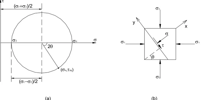
By plotting the corresponding values of σ and τ in a diagram, a circle is obtained with a radius of (σ1–σ2)/2 and center located on the σ-axis at (σ1+σ2)/2 (Figure 2.8a; Jaeger and

Cook, 1979, p. 15). This circle is called Mohr’s circle. A point on the Mohr’s circle gives the magnitude of the normal and shear stresses for any plane oriented at an angle θ from the direction of the major principle stress σ1 (Figure 2.8b).

It is seen from Figure 2.8a that the largest value for the shear stress is (σ1–σ2)/2, and occurs

for θ = 45° and θ = 3π/4 = 135°. A special case arises if σ1= –σ2 and the centre of the Mohr’s

circle is located at the origin of the σ−τ co-ordinate system. In this case the maximum shear plane is free of normal stresses and this state of stress is known as pure shear; this condition provides the basis for some of the failure criteria used in metal plasticity. In general, Mohr’s circle is a very useful tool in the analysis of conditions for the rock failure, as will be seen in Chapter 4.

(a) (b)

Figure 2.8. Mohr’s circle and stress components across a plane. (a) Construction of Mohr’s circle. (b) The stress components acting on a plane correspond to a point on Mohr’s circle.

2θ σ1 σ σ2 (σ1+σ2)/2 (σ1−σ2)/2 (σx,τxy) θ σ1 σ1 σ2 σ2 σ τ x y

(23)

13

2.3 Stress analysis in three dimensions

The two-dimensional analysis considers the equilibrium only in two directions, say the x and y directions, and thus three independent stress components (i.e., σx, σy and τxy) are required to specify the state of stress at a point. The general analysis is three-dimensional and involves six independent stress components (i.e., three normal stresses and three shear stresses) in order to describe the state of stress at a point, as discussed previously. The actual values of these components depend on the orientation of the infinitesimal cube. Thus, the directions where the normal stress components have maximum and minimum values should be considered. This takes place when the shear stress components on all the faces of the cube vanish. These directions, therefore, are principle stress axes, and the stress tensor at the point will have the following simple form:

1 2 3 0 0 0 0 , 0 0 σ σ σ σ ⎛ ⎞ ⎜ ⎟ = ⎜ ⎟ ⎜ ⎟ ⎝ ⎠ (2.17)

where σ1 is the maximum principal stress, σ2 is the intermediate principle stress, and σ3 is the

minimum principle stress (i.e., σ1≥ σ2 ≥ σ3). As a result, there are three principle stresses and

their orientations that must be determined in order that the state of stress at a point is defined. In three-dimensional analysis, a direction in space is identified by the direction cosines (Figure 2.9):

x cos x, y cos y, z cos z,

λ = α λ = α λ = α (2.18)

where αx, αy and αz are the angles between the chosen direction and the x-, y- and z-axes, respectively. The vector λ = (λx,λy,λz) is a unit vector in the chosen direction, and so

2 2 2 _1.

x y z

λ +λ +λ = (2.19)

The principle stresses can be found by solving the following determinant equation for σp (Goodman, 1989, p. 403): 0. x p xy xz xy y p yz xz yz z p σ σ τ τ τ σ σ τ τ τ σ σ − − = − (2.20)

This will give a cubic equation:

3 2

1 2 3 0,

p I p I p I

σ − σ − σ − = (2.21)

(24)

1 2 2 2 2 2 2 2 3 , , 2 . x y z x y y z z x xy yz zx x y z xy yz zx x yz y zx z xy I I I σ σ σ σ σ σ σ σ σ τ τ τ σ σ σ τ τ τ σ τ σ τ σ τ = + + = + + − − − = + − − − (2.22) αy αz αx y x λ∧

Figure 2.9. Direction cosines.

The three solutions of this equation are the principal stresses σ1, σ2 and σ3 (i.e., the

eigenvalues). The quantities I1, I2 and I3 are called stress invariants, which are uniquely

defined regardless of the choice of the co-ordinate axes.

The direction cosines λ1x, λ1y and λ1z identifying the principle axis corresponding to σ1 are

found by the solution of the equations (Jaeger and Cook, 1979, p. 20):

1 1 1 1 1 1 1 1 1 1 1 1 ( ) 0, ( ) 0, ( ) 0. x x y xy z xz x xy y y z yz x xz y yz z z λ σ σ λ τ λ τ λ τ λ σ σ λ τ λ τ λ τ λ σ σ − + + = + − + = + + − = (2.23)

Similarly, the principle axes corresponding to σ2 and σ3 are found by the solution of the

following equations: 2 2 2 2 2 2 2 2 2 2 2 2 ( ) 0, ( ) 0, ( ) 0. x x y xy z xz x xy y y z yz x xz y yz z z λ σ σ λ τ λ τ λ τ λ σ σ λ τ λ τ λ τ λ σ σ − + + = + − + = + + − = (2.24) 3 3 3 3 3 3 3 3 3 3 3 3 ( ) 0, ( ) 0, ( ) 0. x x y xy z xz x xy y y z yz x xz y yz z z λ σ σ λ τ λ τ λ τ λ σ σ λ τ λ τ λ τ λ σ σ − + + = + − + = + + − = (2.25)

Consequently, Eqs. (2.21-2.25) provide the principal stresses and their orientations at a point, which is adequate to specify the state of stress in three dimensions. If the co-ordinate system is oriented so that the x-axis is parallel to the first principal axis, the y-axis parallel to the second and the z-axis parallel to the third, the stress tensor will take the form presented in Eq.

(25)

15

(2.17). Relative to this set of co-ordinate axes, the stresses σ and τ in a general direction λ1, λ2 and λ3 are determined by (Fjaer et al., 1992, p. 12):

2 2 2 1 1 2 2 3 3 2 2 2 2 2 2 2 2 1 1 2 2 3 3 , . λ σ λ σ λ σ σ λ σ λ σ λ σ σ τ + + = + + = + (2.26)

Eq. (2.26) can then be utilized to construct the Mohr’s circle in three dimensions. Consider the plane in the cube in Figure 2.10a. For this plane λ3 = 0, and so the normal and shear

components (σ and τ) on the plane are not affected by σ3, but by σ1 and σ2, and σ and τ are

located on the circle spanning from σ2 to σ1 as shown in Figure 2.10b (i.e., σ1–σ2 Mohr’s

circle). If the plane was perpendicular to σ1, that is, λ1 = 0, then the relationship between σ

and τ can be plotted on the σ2 –σ3 Mohr’s circle. Similarly, if λ2 = 0, σ and τ are located on

the σ1–σ3 Mohr’s circle. For all other directions, the stress conditions lie in the shaded region

between the circles in Figure 2.10b.

σ1 σ2 σ3 θ σ1 σ2 σ3 σ τ (a) (b)

Figure 2.10. Mohr’s circle for three dimensional state of stress. 2.3.1 Octahedral stress

The direction for which the plane in Figure 2.10a is equally inclined to the principal axes, that is 1 2 3 1 , 3 λ λ= =λ = (2.27)

is called the octahedral plane, since it is parallel to a face of an octahedron with vertices on the principal axes. The normal and shear stresses acting on this plane are called the octahedral normal stress (σoct) and the octahedral shear stress (τoct). By substituting Eq. (2.27) in Eq. (2.26), the octahedral normal stress is found to be given by

(26)

1 2 3 1 1 1 ( ) . 3 3 oct I σ = σ σ+ +σ = (2.28)

To determine the octahedral shear stress, introduce Eq. (2.27) into (2.26) to give

2 2 2 1 2 2 3 3 1 1 ( ) ( ) ( ) , 3 oct τ = σ σ− + σ −σ + σ σ− (2.29) or 2 2 2 1 2 3 1 2 2 3 3 1 2 , 3 oct τ = σ +σ +σ −σ σ −σ σ σ σ− (2.30)

which can be written in terms of stress invariants as

1 2 2 1 2 2 ( 3 ) . 3 oct I I τ = − (2.31) 2.3.2 Deviatoric stress

The octahedral normal stress (σoct) defined in Eq. (2.28) is apparently the mean normal stress (σm) which remains unaltered during any change of co-ordinate axes, that is, the invariant I1/3. The mean normal stress is also known as the spherical or hydrostatic stress. It

essentially causes uniform compression or dilatation. In contrast, distortion is essentially determined by the so-called deviatoric stress (stress deviator or stress deviation). The deviatoric stress (s) estimates the deviation of stress from the mean normal stress by subtracting σm from the normal stress components:

. x xy xz x m xy xz xy y yz xy y m yz xz yz z xz yz z m s s s s s s s s s σ σ τ τ τ σ σ τ τ τ σ σ ⎡ ⎤ ⎡ − ⎤ ⎢ ⎥ ⎢ ⎥ =_⎢ _{⎥ ⎢}= − _⎥ ⎢ ⎥ ⎢ ₋ ⎥ ⎣ ⎦ ⎣ ⎦ s (2.32)

The principal axes of the deviatoric stress will be the same as those of stress. The deviatoric principle stresses (s1,s2,s3) can be established from the principle stresses and the spherical

stress, and is given by

1 1 1 2 3 2 2 2 1 3 3 3 3 1 2 (2 ) / 3, (2 ) / 3, (2 ) / 3, m m m s s s σ σ σ σ σ σ σ σ σ σ σ σ σ σ σ = − = − − = − = − − = − = − − (2.33) where s1 ≥ s2 ≥ s3.

Many failure criteria are concerned with distortion. As these criteria must be independent of the choice of co-ordinate axes, the invariants of the deviatoric stress will be involved in failure criteria. These will be denoted by J1, J2, and J3 and are found to be (Jaeger and Cook,

(27)

Basic theory of stress 17 1 x y z 2 2 2 2 x y y z z x xy yz zx 2 2 2 3 x y z xy yz zx x yz y zx z xy J s s s 0, J (s s s s s s ) s s s , J s s s 2s s s s s s s s s . = + + = = − + + + + + = + − − − (2.34)

Using the above equations and rearranging, the octahedral shear stress can be given as

1 2 2 (2 / 3) oct J τ = . (2.35)

(28)

(29)

Stresses around boreholes

19

3

Stresses around boreholes

Underground formations are subjected to a vertical compressive stress caused by the weight of the overlying strata, and horizontal stresses due to the confining lateral restraints. Under the action of these in situ stresses, prior to drilling a borehole, the rock mass is in a state of equilibrium that will be destroyed by the excavation. When a borehole is drilled, the load carried by the removed rock is then taken by the adjacent rock to re-establish equilibrium. As a result, a stress concentration is produced around the well, and so the in situ stresses are modified. If there is no support pressure introduced into the borehole, failure in the formation may take place. Therefore, maintaining equilibrium in the field to prevent rock failure requires the use of a support pressure which is usually provided by a pressurized fluid called “mud”.

To assess the potential mechanical instability of a borehole, a constitutive model is needed in order to know the magnitude of the stresses around a borehole. The literature is rich with such constitutive models. Westergaard (1940) published one of the early works contributing to the knowledge of stress distribution around a borehole, in which an elasto-plastic model was developed. After that, many works using elasto-plastic models have been published (e.g., Gnirk, 1972; Risnes and Bratli, 1981; Mitchell et al., 1987; Anthony and Crook, 2002). On the other hand, there have been other efforts to develop a linear elastic constitutive model (e.g., Paslay and Cheatham, 1963; Fairhurst, 1965b; Bradley, 1979; Aadnoy, 1989b). Out of the numerous published models, linear elastic analysis may be the most common approach. This is due to its requirement of fewer input parameters comparing to other more intricate models.

For instance, Risnes and Bratli (1981), and McLean and Addis (1990a) recommended the use of elasto-plastic model in wellbore stability analysis. Some of those authors, however, in other publications (McLean and Addis, 1990b; Svennekjaer and Bratli, 1998), applied a linear elastic model to carry out the stability analysis for field cases. In practice, the required input data for sophisticated models are rarely available (e.g., Maury and Sauzay, 1987; Fuh et al., 1988; Fleming et al., 1990; Woodland, 1990; Garrouch and Ebrahim, 2001).

Consideration of anisotropic elastic behaviour will further complicate the stability analysis, and many more input parameters will be required. Moreover, the critical mud pressures are not significantly affected by elastic anisotropy for commonly encountered oilfield rocks (Aadnoy, 1988; Aadnoy, 1989a; Chen et al., 1996; Tan et al., 1999; Chen et al., 2002). Therefore, for wellbore stability analysis, we assume that rocks obey isotropic elastic behaviour. In this chapter, an isotropic linear elastic constitutive model is described. The model consists of a three dimensional analyses of stress concentration around an arbitrarily oriented borehole, due to anisotropic in situ stress combined with internal wellbore pressure.

(30)

3.1 Stresses in cylindrical co-ordinates

A cylindrical co-ordinate system is the most convenient system for studying the state of stress around boreholes. Cartesian (x,y,z) and cylindrical (r,θ,z) co-ordinate systems are shown in Figure 3.1. The co-ordinate transformation between Cartesian and cylindrical co-ordinates is defined by the following equations:

_r₌(_x2 ₊_y2)1/2, _θ ₌arctan(_y/_x)._(3.1) and . sin , cosθ y r θ r x= = (3.2) y' z' x' r z θ σr σθ σrθ θ y' x' z' (a) (b)

Figure 3.1. Transformation between Cartesian and cylindrical co-ordinates. (a) Rotation about z′-axis. (b) Stresses in cylindrical co-ordinates.

In the cylindrical co-ordinate system, at any point, the stress tensor becomes

, r r rz r z rz z z θ θ θ θ θ σ σ σ σ σ σ σ σ σ ⎛ ⎞ ⎜ ⎟ ⎜ ⎟ ⎜ ⎟ ⎝ ⎠ (3.3)

where σr is called the radial stress, σθ the tangential stress, and σz the axial stress. Note that the same designation σ is used for all the stress components. This notation will be adopted in this chapter and the following ones. These stresses can be related to the Cartesian co-ordinate stresses by the aid of stress transformation equation, that have the general form (Harrison and Hudson, 2000, p. 50) ' ' ' ' ' ' ' ' ' ' ' ' ' ' ' ' ' ' ' ' ' ' ' ' ' ' ' ' ' ' ' ' ' , x xy xz xx xy xz x x y x z xx xy xz yx y yz yx yy yz y x y y z yx yy yz zx zy z zx zy zz z x z y z zx zy zz σ σ σ λ λ λ σ σ σ λ λ λ σ σ σ λ λ λ σ σ σ λ λ λ σ σ σ λ λ λ σ σ σ λ λ λ ⎛ ⎞ ⎛ ⎞⎛ ⎞⎛ ⎞ ⎜ ⎟ ⎜₌ ⎟⎜ ⎟⎜ ⎟ ⎜ ⎟ ⎜ ⎟⎜ ⎟⎜ ⎟ ⎜ ⎟ ⎜ ⎟⎜ ⎟⎜ ⎟ ⎝ ⎠ ⎝ ⎠⎝ ⎠⎝ ⎠ T (3.4)

where the stress components on the right-hand side of this expression are assumed known, that is, in the (x′,y′,z′) co-ordinate system, and are required in the (x,y,z) co-ordinate system that is inclined with respect to the first. The transformation from (x′,y′,z′) to (x,y,z) is

(31)

21

described by the direction cosines (λxx′,λxy′,λxz′), etc. The term λxx′, for instance, is the

direction cosine of the angle between the x-axis and x′-axis.

The first matrix on the right-hand side of the equation is called the rotation matrix, and the last matrix is its transpose. The transformation from (x′,y′,z′) to (r,θ,z) can be obtained by a rotation θ around the z′-axis, as shown in Figure 3.1. The corresponding rotation matrix is

cos sin 0 sin cos 0 . 0 0 1 θ θ θ θ ⎛ ⎞ ⎜₋ ⎟ ⎜ ⎟ ⎜ ⎟ ⎝ ⎠ (3.5)

Proceeding with the matrix multiplication on the right hand side of the stress transformation equation, using the above rotation matrix, and replacing the matrix on the left-hand side by Eq. (3.3), produces the following formulae for the stress components in cylindrical co-ordinate: 2 2 ' ' ' ' 2 2 ' ' ' ' ' 2 2 ' ' ' ' ' ' ' ' ' ' ' '

cos sin 2 sin cos ,

sin cos 2 sin cos ,

,

( )sin cos (cos sin ),

cos sin , cos sin . r x y x y x y x y z z r y x x y rz x z y z z y z x z θ θ θ σ σ θ σ θ σ θ θ σ σ θ σ θ σ θ θ σ σ σ σ σ θ θ σ θ θ σ σ θ σ θ σ σ θ σ θ = + + = + − = = − + − = + = − (3.6)

3.2 Stresses around deviated boreholes

In this section, the stresses around a deviated borehole with anisotropic horizontal stresses are described. Assume that the in situ principal stresses are vertical stress σv, major horizontal stress σH, and minor horizontal stress σh. These stresses are associated with the co-ordinate system (x′,y′,z′), as illustrated in Figure 3.2a. The z′-axis is parallel to σv, x′-axis is parallel to

σH, and y′-axis is parallel to σh.

These virgin formation stresses should be transformed to another co-ordinate system (x,y,z), to conveniently determine the stress distribution around a borehole. Figure 3.2b shows the (x,y,z) co-ordinate system, where the z-axis is parallel to the borehole axis, the x-axis is parallel to the lowermost radial direction of the borehole, and the y-axis is horizontal. This transformation can be obtained by a rotation α around the z′-axis, and then a rotation i around the y′-axis (Figure 3.3).

(32)

(a) (b)

Figure 3.2. In situ stress co-ordinate system.

Figure 3.3. Stress transformation system for deviated borehole.

The direction cosines associated with the z-axis can be determined by the projection of a unit vector parallel to the z-axis onto the (x′y′z′) axes. This results in

' cos sin , ' sin sin , ' cos .

zx i zy i zz i

λ = α λ = α λ = (3.7)

For the direction cosines associated with the x-axis, the result will be the same as Eq. (3.5), with i by i+( / 2)π , so that

σ

H x

′

i

α

x y

θ

z

′

y

′

σ

h v z

y

x

z

′

x

′

y

′

σ

Η

σ

h v θ

(33)

23

' cos cos , ' sin cos , ' sin .

xx i xy i xz i

λ = α λ = α λ = − (3.8)

Finally, the y-axis is horizontal and makes angles α and α π+( / 2) with the x′ and y′-axes, respectively. Therefore the direction cosines associated with the y-axis are

' sin , ' cos , ' 0.

yx yy yz

λ = − α λ = α λ = (3.9)

These nine direction cosines will form the rotation matrix

cos cos sin cos sin

sin cos 0 ,

cos sin sin sin cos

i i i i i i α α α α α α − ⎛ ⎞ ⎜ ₋ ⎟ ⎜ ⎟ ⎜ ⎟ ⎝ ⎠ (3.10)

and together with the known stress tensor

0 0 0 0 , 0 0 H h v σ σ σ ⎛ ⎞ ⎜ ⎟ ⎜ ⎟ ⎜ ⎟ ⎝ ⎠ (3.11)

using the stress transformation equation, the virgin formation stresses expressed in the (x,y,z) co-ordinate system become:

2 2 2 2

2 2

2 2 2 2

2 2

( cos sin ) cos sin ,

sin cos ,

( cos sin )sin cos ,

0.5( )sin 2 cos ,

0.5( )sin 2 sin ,

0.5( cos sin )sin 2 .

o x H h v o y H h o z H h v o xy h H o yz h H o xz H h v i i i i i i i σ σ α σ α σ σ σ α σ α σ σ α σ α σ σ σ σ α σ σ σ α σ σ α σ α σ = + + = + = + + = − = − = + − (3.12)

The superscript “o” on the stresses denotes that these are the virgin formation stresses. As mentioned before, the excavation of a wellbore will alter the in situ stresses that are given in the above equation. The complete stress solutions, in cylindrical co-ordinate system, around an arbitrarily oriented wellbore are (Hiramatsu and Oka, 1968; Fairhurst, 1968):

(34)

2 4 2 2 4 2 4 2 2 4 2 2 2 4 2 4 4 4 1 1 3 4 cos 2 2 2 1 3 4 sin 2 , 1 1 3 cos 2 2 2 1 3 sin 2 o o o o x y x y r o xy w o o o o x y x y o xy a a a r r r a a a P r r r a a r r a P r θ σ σ σ σ σ θ σ θ σ σ σ σ σ θ σ θ ⎛ + ⎞⎛ ⎞ ⎛ − ⎞⎛ ⎞ =_⎜⎜ _⎟⎟⎜ − ⎟+_⎜⎜ ⎟_⎟⎜ + − ⎟ ⎝ ⎠ ⎝ ⎠ ⎝ ⎠ ⎝ ⎠ ⎛ ⎞ + _⎜ + − _⎟ + ⎝ ⎠ ⎛ + ⎞⎛ ⎞ ⎛ − ⎞⎛ ⎞ =⎜_⎜ ⎟_⎟_⎜ + _⎟−⎜_⎜ ⎟_⎟_⎜ + _⎟ ⎝ ⎠ ⎝ ⎠ ⎝ ⎠ ⎝ ⎠ ⎛ ⎞ − _⎜ + _⎟ − ⎝ ⎠

(

)

(

)

(

)

2 2 2 2 2 2 4 2 4 2 4 2 4 2 2 2 2 2 , 2 cos 2 4 sin 2 , 1 3 2 sin 2 1 3 2 cos 2 , 2 sin cos 1 , cos sin 1 w o o o o z z x y xy o o x y o r xy o o z xz yz o o rz xz yz a r a a r r a a a a r r r r a r a r θ θ σ σ ν σ σ θ σ θ σ σ σ θ σ θ σ σ θ σ θ σ σ θ σ θ ⎡ ⎤ = − _⎢ − + _⎥ ⎣ ⎦ ⎡ ⎛ − ⎞⎛ ⎞ ⎤ ⎛ ⎞ = −⎢ ⎜_⎜ ⎟⎜_⎟ − + ⎟ ⎥+ ⎜ − + ⎟ ⎢ ⎝ ⎠⎝ ⎠ ⎥ ⎝ ⎠ ⎣ ⎦ ⎛ ⎞ = − + _⎜ + _⎟ ⎝ ⎠ ⎛ = + − ⎝ , ⎞ ⎜ ⎟ ⎠ (3.13)

where “a” is the radius of the wellbore, Pw is the internal wellbore pressure, and ν is a material constant called Poisson’s ratio. The angle θ is measured clockwise from the x-axis, as shown in Figure 3.3.

Eq. (3.13) is derived under the assumption that there is no displacement along the z-axis, that is, a plain strain condition, in order to estimate σr, σθ, σz and σrθ. The longitudinal shear

stresses, σθz and σrz, however, are determined assuming that all plane sections normal to the z-axis undergo the same deformations as a result of longitudinal shears. The equations for stresses around a circular opening were first published by Kirsch (1898), where the opening is assumed to be parallel to a principle stress axis (Charlez, 1991, p. 87). The stress field around a circular opening in any direction was first presented by Hiramatsu and Oka (1968) and Fairhurst (1968).

3.3 Stresses at borehole wall in anisotropic stress field

In a linear elastic material, the largest stress concentration occurs at the borehole wall. Therefore, borehole failure is expected to initiate there. For wellbore instability analysis, consequently, stresses at the borehole wall are the ones that should be compared against a failure criterion. These stresses are determined for deviated, vertical and horizontal wellbores in the following sections.

(35)

25

3.3.1 Deviated wellbore

For deviated wellbore, the stresses at borehole wall are estimated by setting r = a in Eq. (3.13), which gives

(

)

(

)

(

)

, 2 cos 2 4 sin 2 , 2 cos 2 4 sin 2 , 2 sin cos , 0, 0. r w o o o o o x y x y xy w o o o o z z x y xy o o z xz yz r rz P P θ θ θ σ σ σ σ σ σ θ σ θ σ σ ν σ σ θ σ θ σ σ θ σ θ σ σ = = + − − − − ⎡ ⎤ = − _⎣ − + _⎦ = − + = = (3.14) 3.3.2 Vertical wellbore

In order to determine the stresses at wall of a vertical borehole, we set the inclination angle i = 0 in Eq. (3.12). For simplicity, we orient the horizontal axes so that the direction θ = 0 is parallel to σH (i.e., α = 0), as shown in Figure 3.4. Consequently, the stresses become

(

)

(

)

, 2 cos 2 , 2 cos 2 , 0, 0, 0. r w H h H h w z v H h z r rz P P θ θ θ σ σ σ σ σ σ θ σ σ ν σ σ θ σ σ σ = = + − − − = − − = = = (3.15) x′ θ z′ y′ σh v σH

(36)

3.3.3 Horizontal wellbore

To estimate the stresses at the wall of a horizontal borehole, we put i = π/2 in Eq. (3.12), which gives 2 2 2 2 , sin cos , cos sin , 0, 0.5( )sin 2 , 0. o x v o y H h o z H h o xy o yz h H o xz σ σ σ σ α σ α σ σ α σ α σ σ σ σ α σ = = + = + = = − = (3.16)

Introducing Eq. (3.16) into Eq. (3.14), the stresses at borehole wall will be

(

) (

)

(

)

2 2 2 2

,

sin cos 2 sin cos cos 2 ,

cos sin 2 sin cos cos 2 ,

( )sin 2 cos , 0, 0. r w v H h v H h w z H h v H h z h H r rz P P θ θ θ σ σ σ σ α σ α σ σ α σ α θ σ σ α σ α ν σ σ α σ α θ σ σ σ α θ σ σ = = + + − − − − = + − − − = − = = (3.17)

Figure 3.5 illustrates the stress transformation system corresponding to a horizontal wellbore. In this configuration, notice that the angle θ is measured anticlockwise from the x-axis.

σH x′ α x y θ z′ y′ σh σv z

(37)

27

For the case in which the wellbore axis lies along the maximum horizontal principal stress (i.e., α = 0), the stresses at borehole wall are

(

)

(

)

, 2 cos 2 , 2 cos 2 , 0, 0, 0, r w v h v h w z H v h z r rz P P θ θ θ σ σ σ σ σ σ θ σ σ ν σ σ θ σ σ σ = = + − − − = − − = = = (3.18)

which are identical to those given by the Kirsch solution (see Obert and Duvall, 1967, p. 99; Charlez, 1997, p. 64, for example).

3.4 Stress variation

According to the equations obtained in the previous section, tangential stress (σθ) and axial

stress (σz) are functions of the angle θ. This angle indicates the orientation of the tangential stress around the wellbore circumference, varies from 0 to 360 degrees. Consequently, the tangential and axial stresses will vary sinusoidally.

Consider a typical wellbore in a reservoir which has wellbore pressure Pw = 5000 psi, Poisson’s ratio ν = 0.25, and in situ stresses of σv = 12,000 psi, σH = 10,000 psi and σh = 9,000 psi. For a vertical wellbore, both tangential and axial stresses reach a maximum value (i.e., σθmax = 16,000 psi and σzmax = 12,500 psi) at θ = ±π/2, and the minimum value (i.e.,

σθmin = 12,000 psi and σzmin= 11,500 psi) at θ = 0 or π, as shown in Figures 3.4 and 3.5. These critical positions remain the same for any values of the in situ stresses (i.e., σv, σH and σh). Furthermore, if the horizontal stresses are equal, then σθ and σz are constant and independent of the angle θ.

Similarly, for a horizontal wellbore, the critical positions of σθ and σz are θ = ±π/2 and θ = 0 or π. The largest or smallest values of σθ (or eventually σz) will occur at either of these two positions, depending up on the values of the in situ stresses. If σH > σh > σv, for instance, the largest and smallest σθ occur at θ = 0 or π and θ = ±π/2, respectively. For a deviated

borehole, however, there is no particular a priori angle at which σθ and σz reach the maximum or minimum value. This results in complicating the borehole stability analysis for non-vertical boreholes, which will be discussed in subsequent chapters.

(38)

12000 16000

0 90 180 270 360

θ σθ

Figure 3.6. Tangential stress variation at the wall of a vertical borehole.

11500 12500 0 90 180 270 360 θ σ z

(39)

Rock failure criteria

29

4

Rock failure criteria

The rock mechanics literature is rich with a number of failure criteria that have been developed. Among these criteria, Mohr-Coulomb criterion is much referred to and used in practice. This criterion involves only the maximum and minimum principal stresses, σ1 and σ3. It implicitly assumes that σ2 has no influence on rock strength. In general, the

independence of rock failure on σ2 is a common assumption in failure criteria (Pan and

Hudson, 1988; Aubertin et al., 2000; Yu et al., 2002). The situation in which σ2 = σ3 is a

special case that may be encountered in situ (Haimson, 1978; McGarr and Gay, 1978). For a polyaxial stress state, in which σ2 > σ3, the intermediate principal stress has a pronounced

effect. In contrast to the prediction of Mohr-Coulomb criterion, experimental work by Murrell (1963), Handin et al. (1967), Hoskins (1969), Mogi (1967; 1971b), Michelis (1985; 1987a), Reik and Zacas (1978), Wawersik et al. (1997), Tiwari and Rao (2004), Haimson and Chang (2000; 2002; 2005), and others, has demonstrated that rock strength is higher when σ2

> σ3.

Numerous researchers have faced situations in which the Mohr-Coulomb criterion was found deficient. Vernik and Zoback (1992), for instance, found that the use of Mohr-Coulomb criterion in relating borehole breakout dimensions to the in situ stress conditions in crystalline rocks did not provide realistic results. Therefore, they recommended the use of a failure criterion that accounts for the influence of σ2 on rock strength, to represent rock conditions

more realistically. Song and Haimson (1997) conducted laboratory tests of borehole breakouts in Westerly granite and Berea sandstone, and compared the observed breakouts with different failure criteria. They concluded that Mohr-Coulomb criterion is not applicable to the analysis of breakout formation, whereas criteria that include the strengthening effect of

σ2, such as the Mogi criterion, were much more in agreement with the experimental

observations. Single et al. (1998) pointed out that the effect of σ2 is important in underground

excavation, and so, they suggested a modification for Mohr-Coulomb criterion. Ewy (1998; 2001) and Kristiansen (2004) concluded that for the purpose of calculating the critical mud weight required to maintain wellbore stability, Mohr-Coulomb is too conservative due to the ignoring the strengthening effect of σ2. Yi et al. (2005) reported that the onset of sand

production can not be properly predicted by adopting Mohr-Coulomb criterion.

There are a number of numerical models that highlight the impact of σ2 on rock strength. For

example, Zhou (1994) developed a numerical model to determine the borehole breakout dimensions based on various rock failure criteria. He found that Mohr-Coulomb criterion tends to predict larger breakouts than those predicted by other criteria that take into account the effect of σ2. Recently, Fjaer and Ruistuen (2002) developed a numerical model simulating

rock failure tests for a granular material. Their simulations showed that σ2 has an impact on

rock strength that is in agreement with several previously published experimental data. In order to consider the impact of σ2 on strength, several 3D rock failure criteria have been

(40)

investigate the impact of σ2 on rock strength. They derived a failure criterion by calculating

the shear strain energy associated with microcracks in the material. The criterion requires the knowledge of the coefficient of sliding friction between crack surfaces, a parameter that cannot be determined experimentally. Therefore, numerical methods are required for practical use of the criterion. Desai and Salami (1987) introduced a 3D failure criterion that requires more than six input parameters, and Michelis (1987b) proposed another criterion in which four constants are involved (see Pan and Hudson, 1988; Hudson and Harrison, 1997, p. 112). In general, the 3D failure criteria are usually difficult in practice to apply, particularly for wellbore stability problems. In wellbore stability analysis, when the influence of σ2 on rock

failure characteristics is considered, the Drucker-Prager failure criterion is often implemented (Marsden et al., 1989; McLean and Addis, 1990a). This failure criterion, however, has been reported to overestimate the intermediate principal stress effect, which may result in nonsensical stability predictions (McLean and Addis, 1990b; Ewy, 1999). Moreover, the Drucker-Prager criterion disagrees with the Mogi failure criterion, which considers the effect of σ2 based on true triaxial tests (i.e., polyaxial tests). The fundamental difference between

these two criteria is elaborated upon later in this chapter.

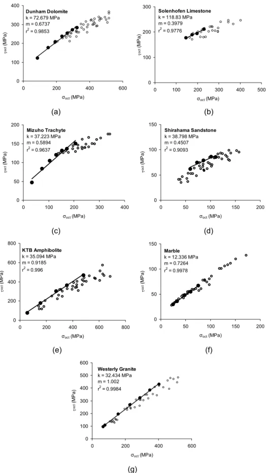
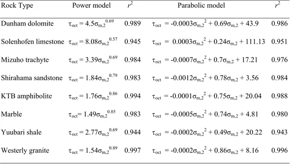
The usefulness of the Mogi failure criterion remains the subject of debate (Haimson and Chang, 2000; Colmenares and Zoback, 2002). In particular, the power-law form of the Mogi criterion has been criticised because its two parameters cannot be related to the standard parameters of the Coulomb failure law, such as the cohesion and the angle of internal friction. In this chapter, we first review and define a number of failure criteria that are commonly used in rock mechanics. We then examine published data from eight rocks, and show that a linear form of the Mogi criterion does a good job of representing polyaxial failure data. After that, the possibility of estimating Mogi strength parameters from triaxial test data is examined. In addition, we compare the Drucker-Prager criterion with polyaxial test data for a variety of lithologies, in order to assess its applicability in representing failure under polyaxial stress states.

4.1 Coulomb criterion

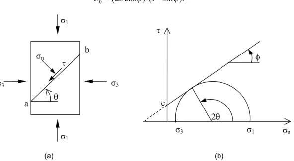
In 1776, Coulomb introduced the simplest and most important criterion. He suggested that rock failure in compression takes place when the shear stress, τ, that is developed on a specific plane (plane a-b in Figure 4.1(a), for example) reaches a value that is sufficient to overcome the natural cohesion of the rock, as well as the frictional force that opposes motion along the failure plane. The criterion can be written as

tan ,τ = +c σ_n φ (4.1) where σn is the normal stress acting on the failure plane (plane a-b in Figure 4.1(a)), c is the cohesion of the material and φ is the angle of internal friction. Figure 4.1(b) shows the strength envelope of shear and normal stresses. As the sign of τ only affects the direction of sliding, Eq. (4.1) should be written in terms of |τ|, but for simplicity we will omit the absolute value sign.

As criteria (4.1) will always first be satisfied on a plane that lies in the direction of σ2, the

value of σ2 will not influence σn or τ, and so this failure criterion implicitly assumes that σ2

has no effect on failure. Alternatively, this criterion can be interpreted as being intended to apply only to situations in which σ2 = σ3. The Coulomb failure criterion, therefore, can be

(41)

Rock failure criteria

31

represented by the maximum principal stress, σ1, and minimum principal stress, σ3. By

applying Eqs. (2.10,2.11), one can obtain

1 3 1 3 1 1 ( ) ( ) cos 2 , 2 2 n σ = σ σ+ + σ σ− θ (4.2) and 1 3 1 ( )sin 2 , 2 τ = σ σ− θ (4.3)

where θ is the angle between the normal to the plane and the direction of the maximum principal stress (Figure 4.1(a)). From Figure 4.1(b), we find that

. 4 2

π φ

θ = + (4.4)

Using Eqs. (4.2-4.4), Coulomb criterion given by Eq. (4.1) can be written as

1 C0 q 3,

σ = + σ (4.5)

where q is the slope of the line relating σ1 and σ3, and is given by

tanq= ψ = +(1 sin ) /(1 sin ),φ − φ (4.6) where ψ is the angle of the slope of the line relating σ1 and σ3 (Figure 4.2), and C0 is the uniaxial compressive strength, which can be related to the cohesion and the angle of internal friction by

0 (2 cos ) /(1 sin ).

C = c φ − φ (4.7)

(a) (b)

Figure 4.1. Coulomb failure criterion. (a) Shear failure on plane a-b. (b) Strength envelope in terms of shear and normal stresses.

σ1 θ σ1 σ3 σ3 σn τ b a 2θ σn τ σ1 σ3 c φ

(42)

Figure 4.2. Coulomb strength envelope in terms of principal stresses.

From Eqs. (4.5-4.7), we find that the uniaxial tensile strength, T0, is given in terms of c and φ

as

0 (2 cos ) /(1 sin ).

T = c φ + φ (4.8) The true uniaxial tensile strength takes values, T0true, that are generally lower than those

predicted by Eq. (4.8) (Brady and Brown, 1999). Consequently, a tensile cut-off is usually applied at T0true, as shown in Figure 4.3. In practical rock mechanics use, it is prudent to put

T0true = 0 (Bradley, 1979; Brady and Brown, 1999; Zhao, 2000).

Figure 4.3. Coulomb strength envelopes with a tensile cut-off.

The Coulomb criterion can also be expressed in terms of the maximum shear stress, τmax, and the effective mean stress, σm,2 (Jaeger and Cook,1979, p.98):

max ccos sin m,2,

τ = φ+ φσ (4.9) where max 1 3 1 ( ), 2 τ = σ σ− (4.10) 1 3 ,2 ( ). 2 m σ σ σ = + (4.11)

From this form of the Coulomb failure criterion, we can conclude that (a) the mean normal stress inhibits the creation of a failure plane is σm,2, and (b) there is predicted to be a linear relationship between the maximum shear stress and the effective mean stress at failure.

σ1 σ3 ψ C0 τ φ σ1 ψ σ3 σn T0true T0true

Wellbore stability analysis based on a new true-triaxial failure criterion

W

ELLBORE

S

TABILITY

A

NALYSIS

B

ASED ON A

N

EW

T

RUE

-T

RIAXIAL

F

AILURE

C

RITERION

Adel Al-Ajmi

Abstract

Acknowledgments

Table of contents

1

Introduction

2

Basic theory of stress

σ

σ

τ

τ

σ

σ

τ

τ

σ

τ

σ

τ

3

Stresses around boreholes

σ

′

α

θ

′

′

σ

y

x

z

z

′

x

′

y

′

σ

σ

(

)

(

)

(

)

(

)

(

)

(

)

(

)

(

)

(

) (

)

(

)