Recurrent neural networks in electricity load forecasting

Recurrent neural networks in

electricity load forecasting

SAMIUL ALAM

KTH ROYAL INSTITUTE OF TECHNOLOGY

electricity load forecasting

SAMIUL ALAM

Master in Computer Science Date: August 14, 2018 Supervisor: Pawel Herman Examiner: Hedvig Kjellström

Principal: Mattias Jonsson, Expektra

Swedish title: Rekurrenta neurala nätverk i prognostisering av elkonsumtion

Abstract

In this thesis two main studies are conducted to compare the predic-tive capabilities of feed-forward neural networks (FFNN) and long short-term memory networks (LSTM) in electricity load forecasting.

The first study compares univariate networks using past electricity load, as well as multivariate networks using past electricity load and air temperature, in day-ahead load forecasting using varying lookback periods and sparsity of past observations. The second study compares FFNNs and LSTMs of different complexities (i.e. network sizes) when restrictions imposed by limitations of the real world are taken into con-sideration.

No significant differences are found between the predictive per-formances of the two neural network approaches. However, adding air temperature as extra input to the LSTM is found to significantly decrease its performance. Furthermore, the predictive performance of the FFNN is found to significantly decrease as the network complexity grows, while the predictive performance of the LSTM is found to in-crease as the network complexity grows. All the findings considered, we do not find that there is enough evidence in favour of the LSTM in electricity load forecasting.

Sammanfattning

I denna uppsats beskrivs två studier som jämför feed-forward neurala nätverk (FFNN) och long short-term memory neurala nätverk (LSTM) i prognostisering av elkonsumtion.

I den första studien undersöks univariata modeller som använder tidigare elkonsumtion, och flervariata modeller som använder tidiga-re elkonsumtion och temperaturmätningar, för att göra prognoser av elkonsumtion för nästa dag. Hur långt bak i tiden tidigare informa-tion hämtas ifrån samt upplösningen av tidigare informainforma-tion varieras. I den andra studien undersöks FFNN- och LSTM-modeller med prak-tiska begränsningar såsom tillgänglighet av data i åtanke. Även storle-ken av nätverstorle-ken varieras.

I studierna finnes ingen skillnad mellan FFNN- och LSTM- mo-dellernas förmåga att prognostisera elkonsumtion. Däremot minskar FFNN-modellens förmåga att prognostisera elkonsumtion då storle-ken av modellen ökar. Å andra sidan ökar LSTM-modellens förmåga då storkelen ökar. Utifrån dessa resultat anser vi inte att det finns till-räckligt med bevis till förmån för LSTM-modeller i prognostisering av elkonsumtion.

1 Introduction 1

1.1 Aims and scope . . . 3

1.2 Thesis outline . . . 4

2 Background 5 2.1 Related work . . . 5

2.1.1 ANNs for electricity load or production forecasting 5 2.1.2 Comparison of FFNNs and RNNs in other fields . 7 2.2 Artificial neural networks in time series prediction . . . . 7

2.2.1 FFNN . . . 8 2.2.2 LSTM . . . 10 2.3 Generalization . . . 12 2.3.1 Early stopping . . . 12 2.3.2 Weight decay . . . 13 2.3.3 Dropout . . . 13 3 Methods 14 3.1 Experimental setup . . . 14 3.1.1 Experiment 1 . . . 15 3.1.2 Experiment 2 . . . 17

3.2 Training, validation, and evaluation . . . 19

3.2.1 Data preprocessing . . . 20

3.2.2 Evaluation metrics . . . 20

3.2.3 Model optimization and regularization . . . 20

3.2.4 Statistical hypothesis testing . . . 21

4 Results 22 4.1 Experiment 1 . . . 23

4.2 Experiment 2 . . . 30

5 Discussion 35

5.1 Summary of findings . . . 35 5.2 The effect of adding air temperature as extra input to a

model . . . 36 5.3 The effect of different lookback periods . . . 37 5.4 The effect of network complexity on predictive

perfor-mance . . . 38 5.5 Limitations . . . 39 5.6 Ethics and sustainability . . . 39

6 Conclusion 40

6.1 Future work . . . 41

Introduction

The importance of renewable energy is being recognized by more peo-ple around the world. In the European Union (EU) the Renewable Energy Directive1 _{establishes a policy for the production and}

promo-tion of energy from renewable sources and requires the EU to fulfill at least 20% of its total energy needs with renewable energy by 2020.

Not all renewable energy sources are totally reliable. Intermittency and variability of energy output from sources such as solar energy and wind energy lowers their penetration into our energy systems. These issues can be reduced by forecasting their variation and inte-grating them with dispatchable renewables such as hydropower. Fur-thermore, forecasting the energy demand, a task known as electricity load forecasting, allows for optimal matching of supply and demand which results in higher penetration of renewable power into our en-ergy systems.

Effort has been put into improving the methods for electricity load forecasting. Alfares and Nazeeruddin [1] categorizes and reviews a wide range of methods, discussing advantages and disadvantages of each category and reviewing pertinent literature. They conclude that over the last few years the most active research area has been artificial neural network (ANN) based load forecasting.

Electricity load is a random nonstationary process [1]. Outliers, level shifts, and variance changes are some of the nonstationarities that occur in electricity load time series. An outlier is a data point that is distant from other data points in a dataset. Outliers can occur due to

1

https://ec.europa.eu/energy/en/topics/renewable-energy/renewable-energy-directive

incidental systematic error which means they do not follow the general trend and behaviour of the rest of the data. Therefore naive time se-ries predictions derived from datasets that include outliers can be mis-leading. A level shift is an abrupt and permanent change of the trend level in the time series. Level shifts can occur due to a policy change or a change in technology that shifts the level of electricity consump-tion. Some ANNs such as feed-forward neural networks (FFNNs) that have been trained using data prior to a level shift has no knowledge of the subsequent level shift and can have problems analyzing future observations. In a similar way a sudden change in variance in a time series can also lead to errors in estimates of electricity consumption statistics. These nonstationarities have a detrimental effect on the time series prediction performance of FFNNs [2].

Efforts have been made to classify and mitigate the effects of non-stationarities in electricity load time series in order to improve the pre-diction accuracy of electricity load forecasting models. Tsay [3] de-scribed the problem of detecting outliers, level shifts, and variance changes in univariate time series of air passenger miles and IBM clos-ing stock prices by specifyclos-ing an autoregressive movclos-ing average model and its parameters for the observed series. Virili and Freisleben [2] showed that “the presence of stochastic or deterministic trends in eco-nomic time series can be a major obstacle for producing satisfactory predictions with neural networks”. After demonstrating the effects of nonstationarities on neural networks using the time series of mortgage loans, they also showed that appropriate preprocessing techniques im-prove the prediction quality of neural networks. A certain class of ANNs known as recurrent neural networks (RNNs) were not included in these investigations. This poses the question of whether RNNs can handle nonstationary time series better than other types of neural net-works such as FFNNs without the need for nonstationarity detection and preprocessing techniques.

RNNs have become increasingly popular due to their success in tasks such as image captioning and language processing [4]. Connor et al. [5] showed that RNNs are a special case of nonlinear autoregressive-moving average model and that feed-forward neural networks are a special case of nonlinear autoregressive models. They concluded that they are well-suited for time series that possess moving average com-ponents, are state dependent, or have trends. They also proposed a learning algorithm based on filtering outliers from the data and then

estimating parameters from the filtered data, and showed that recur-rent neural networks can outperform feed-forward neural networks by applying the proposed method to predict electricity load time se-ries from Puget Sound Power and Light Company.

Bianchi et al. [6] did a more recent survey on RNNs in short-term load forecasting which provides an overview and comparative anal-ysis of five different models, the Elman Recurrent Neural Network (ERNN), also known as Simple RNN, the Long Short-Term Memory (LSTM) architecture originally proposed by Hochreiter and Schmidhu-ber [7], the Gated Recurrent Unit (GRU) originally proposed by Cho et al. [8], and two other architectures called the NARX network and Echo State Network (ESN), using three real datasets, the Orange telephone dataset measuring telephonic activity load, and the ACEA dataset and GEFCom2012 dataset both measuring electricity load. They concluded that while while LSTM and GRU achieve outstanding results in many sequence learning problems, no specific model outperformed the oth-ers in every prediction problem in their analysis. However, there is still no conclusive evidence in favour of LSTMs when compared to more classical FFNNs, especially in the context of electrical load forecasting.

1.1 Aims and scope

This work is aimed at a comparative analysis of FFNNs and RNNs in electricity load forecasting. While there are numerous types of RNNs that may be suitable for the problem of electricity load forecasting, this investigation is limited to LSTM networks. Classification of nonsta-tionarities in a time series is out of the scope. They are considered as a bag of nonstationarities occurring in the electricity load time series and other related time series. Benchmark time series provided by Ex-pektra, the company involved in the project, are used to evaluate the models. No additional sources of data are used for the project.

This thesis consists of two main studies. In the first study the FFNN and the LSTM is compared in univariate time series prediction for day-ahead load forecasting. Since many real-world problems combine time series prediction with extra inputs it is also interesting to compare the FFNN and the LSTM in a similar setting. Air temperature has been shown to improve the accuracy of FFNNs (e.g. [9], [10], [11], [12]). Therefore, air temperature is added as additional input to both

mod-els. This allows us to test the models in both univariate and multivari-ate time series prediction.

In the second study we take into consideration some of the restric-tions that are imposed on a prediction system by limitarestric-tions in the real-world. For example, not all data needed for electricity load prediction at a city scale is instantaneously available to the prediction system, in-stead many different measurements are combined to make aggregate data. We compare the FFNN and the LSTM here using a configuration of inputs that are constrained by such restrictions.

1.2 Thesis outline

In chapter 2 the reader is presented with related work and theoretical background on artificial neural networks in electricity load forecast-ing. In chapter 3 the methodology for conducting this study is pre-sented. Chapter 4 contains results from the studies. Chapter 5 contains a summary and discussion of the findings as well as a review on the ethics and sustainability aspects of the thesis. Chapter 6 concludes the thesis with final recommendations and suggestions on future work.

Background

2.1 Related work

2.1.1 ANNs for electricity load or production

forecast-ing

ANNs have been used successfully in electricity load forecasting be-fore. Park et al. [13] used an MLP and regression techniques to forecast electricity load one-hour and 24-hours ahead on data from the Puget Sound Power and Light Company. Lee et al. [14] suggested a nonlinear load model using FFNNs to produce 24-hour ahead forecasts using the past 48 hours of data from Korea Electric Power Company, achieving satisfactory performance.

Weather information is often used in combination with past load to improve forecasting accuracy. Park and Mohammed [9] used an ANN to learn the relationship between load and air temperature to forecast electric peak load. Chen et al. [10] presented a nonfully connected ANN that can differentiate between weekday and weekend loads and forecast hourly loads for an entire week. Furthermore, they demon-strated that ANNs are appropriate when the load curve is a nonlinear function of multiple variables, e.g. past load and weather informa-tion such as air temperature, using data from Wisconsin Electric Power Company. Chen et al. [11] proposed an ANN based model for electric-ity load forecasting and showed that forecasting accuracy is improved when considering the air temperature effect on the energy demand. Al-Fuhaid et al. [12] incorporated air temperature and humidity effects to produce short-term load forecasts of the electrical power system in

Kuwait.

ANNs have also been used in combination with other methods for electricity load or power production forecasting. Mbuvha [15] investi-gated benefits of using Bayesian neural networks in short-term wind power forecasting. Åkerberg [16] addressed the detrimental effect that outliers have on neural networks and showed how machine learning methods for outlier detection improves wind power predictions made by an MLP. Furthermore, Srinivasan and Lee [17] surveyed hybrid fuzzy logic neural network approaches to electricity load forecasting, and Alfares and Nazeeruddin [1] surveyed other hybrid neural net-work approaches for electricity load forecasting, which the reader is encouraged to refer to.

RNNs have been used in electricity load forecasting in numerous ways. Mandal et al. [18] used a simple RNN combined with a pre-processing step to cluster similar days and was able to reliably fore-cast electricity load using hourly load and air temperature data from Okinawa Electric Power Company. Marino et al. [19] proposed an LSTM-based sequence-to-sequence model for electricity load forecast-ing showforecast-ing improvements over a standard LSTM architecture. Cheng et al. [20] proposed an LSTM-based neural network that they described as “the first power demand forecasting model based on LSTM that incorporates time series features, weather features, and calendar fea-tures”. It was compared to a Gradient Boosting Tree model and a Sup-port Vector Regression model using power usage data provided by the University of Masachusetts, and was shown to outperform both mod-els.

However, few comparative analyses of FFNNs and RNNs in the context of electric load or power production forecasting exist. Zheng et al. [21] compared a univariate, LSTM-based neural network to nu-merous methods including NNETAR, “a neural network with lagged values of a time series as inputs”1_{. The LSTM-based network}

outper-formed all other methods in an electricity load forecasting simulation. Svensson [22] investigated the use of artificial neural networks for short-term wind power prediction, comparing FFNNs and recurrent architectures known as Hierchical Temporal Memory/Cortical Learn-ing Algorithms usLearn-ing the GEFCom2012 dataset. The Hierchical Tem-poral Memory/Cortical Learning Algorithm was shown to outper-form the FFNN. Kuo and Huang [23] proposed a Convolutional

ral network (CNN) for electricity load forecasting and compared it to LSTM and MLP based networks. The LSTM-based network outper-formed the MLP while the CNN-based network was best overall.

2.1.2 Comparison of FFNNs and RNNs in other fields

FFNNs and RNNs have been compared in various other fields. The ability of RNNs to process data sequentially makes them appropriate for tasks such as speech recognition. Graves and Schmidhuber [24] compared multiple LSTM-based networks and MLPs in a framewise phoneme classification task, showing that the LSTM models outper-forms MLP models. Weninger et al. [25] used LSTM-based networks to predict speech from noisy speech and showed improvements over conventional FFNNs. Sundermeyer et al. [26] compared an FFNN-based network and an LSTM-FFNN-based network on a French speech recog-nition task, showing that the LSTM outperformed the FFNN approach. Parascandolo et al. [27] showed that LSTM-based networks outper-form FFNNs in polyphonic sound event detection. For more infor-mation the reader is encouraged to refer to Lipton et al. [28] who has reviewed the application of LSTMs in various fields such as natural language processing and translation, image captioning, and handwrit-ing recognition.

2.2 Artificial neural networks in time series

prediction

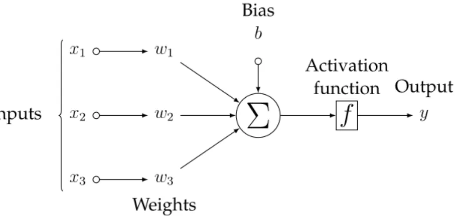
Artificial neural networks consist of a collection of nodes. The way these nodes work is inspired by “the hypothesis that mental activity consists primarily of electrochemical activity in networks of brain cells called neurons” [29]. The basic idea is that a node “fires” when a linear combination of its inputs exceeds some threshold, and the topology and the properties of the neurons determine the properties of a neural network. Figure 2.1 shows a mathematical representation of a node. Each incoming connection to the node has an associated weight, wi,

used by the node to compute a weighted sum of the inputs, xi, together

with a bias term, b. This sum is then passed through an activation function f to produce an output y = f(P3

i=1wixi+ b), where f is some

x2 w2

⌃

f

Figure 2.1: A simple illustration of a neural network node with 3 inputs.

2.2.1 FFNN

The FFNN was the first type of neural network devised. FFNNs are a class of neural networks that consist of multiple layers of nodes that are connected in a feed-forward way such that each node has directed connections to every node in the next layer. The networks are acyclic which means that the information only moves in one direction from the first layer of nodes, the input layer, to the last layer of nodes, the output layer. An FFNN with one or more layers between the input layer and output layer is called a multi-layer perceptron (MLP). The layers between the input and output layers are called hidden layers and the nodes in these layers are called hidden nodes. It has been shown that any real-valued function can be approximated arbitrarily closely by an MLP with just one hidden layer and a fixed number of hidden nodes [30].

Predicting future values of a time series using past observations is commonly referred to as time series prediction. Predicting the value of some time series for the next time step is called one-step ahead pre-diction. Similarly, predicting the k:th step into the future is referred to as k:th-step ahead prediction. At any time step, t, such a predic-tion is denoted as ˆyt+k. It is often assumed that there are temporal

dependencies in a time series. However, FFNNs cannot process a time series sequentially. Instead, they have to be used with time-delayed input representations, treating past observations as independent vari-ables. The networks are then used to learn the relationship between the time-delayed inputs and the target. Figure 2.2 illustrates how an MLP can be used with time-delayed input representations to produce

k:th-step ahead predictions of a time series.

...

...

Figure 2.2: Illustration of an MLP using time-delayed input representation of a time series, [yt l, ..., yt], to produce k:th-step ahead predictions ˆyt+k.

Many different learning methods have been devised for neural works where the goal is to minimize the difference between the net-work’s output, typically denoted as ˆy, and the target, y, defined by some cost or error function such as the mean squared error given in Equation 2.1. M SE = 1 T T X t=1 (yt yˆt)2 (2.1)

The learning methods are commonly based on gradient descent op-timization where the gradient of the error function with respect to the network’s weights is used to make small, iterative adjustments to the weights until a minimum is found. Backpropagation is a popu-lar method for computing the gradients needed to adjust the weights, and works by propagating the error backwards through the network using the chain rule for computing the derivative of composite func-tions. Several variants and extensions of gradient descent make learn-ing more efficient which is helpful for trainlearn-ing neural networks uslearn-ing large volumes of data. Some examples include stochastic gradient

de-scent — and ADAM [31] and RMSProp [32] which are both based on stochastic gradient descent. For more details on MLPs the reader is encouraged to refer to any of the numerous handbooks, e.g. [33].

2.2.2 LSTM

RNNs have connections between their units that form a directed graph along a sequence as illustrated in Figure 2.3. They also have an inter-nal state vector, or memory, and recursively compute new states by ap-plying its activation functions to previous states and new inputs. This allows RNNs to process information sequentially and exhibit tempo-ral behaviour for a time sequence while retaining information from the past.

In order to train an RNN using gradient descent and backpropa-gation the RNN needs to be represented in a way that forms a closed-form relation between the model parameters and the error function. This can be done by unfolding the recurrent neural network and repli-cating its hidden layer structure for a fixed number of timesteps and connecting its recurrent connections in a feed-forward way as illus-trated in Figure 2.3. The replicas represent the recursive application of the same operation which means that the weights in each replica need to be constrained to assume the same values. Now the errors can be propagated through the unfolded RNN and the weights can be adjusted accordingly. This technique for training RNNs is known as backpropagation through time (BPTT) [34].

Figure 2.3: Unfolding of an RNN for a fixed number of timesteps t. Adapted from Olah [35].

Vanilla RNNs have limited memory since the gradients will even-tually vanish or explode when propagating the error back through

time2_{. Gated architectures like the LSTM were designed specifically to}

address this issue by allowing for constant error flow through LSTM cells. Equations 2.2 – 2.7 show how the output of an LSTM network is computed. The way these gates are designed keeps constant error flowing back through time.

forget gate: f[t] = (Wfx[t] + Rfy[t 1] + bf) (2.2)

candidate gate: ˜h[t] = g1(Whx[t] + Rhy[t 1] + bh) (2.3)

update gate: u[t] = (Wux[t] + Ruy[t 1] + bu) (2.4)

cell state: h[t] = u[t] ˜h[t] + f[t] h[t 1] (2.5)

output gate: o[t] = (Wox[t] + Roy[t 1] + bo (2.6)

output: y[t] = o[t] g2(h[t]) (2.7)

“where x[t] is the input vector at time t. Wf, Wh, Wu, and Wo are

rectangular weight matrices, that are applied to the input of the LSTM cell. Rf, Rh, Ru, and Roare square matrices that define the weights of

the recurrent connections, while bf, bh, bu, and boare bias vectors. The

function (·) is a sigmoid, while g1(·) and g2(·) are point-wise

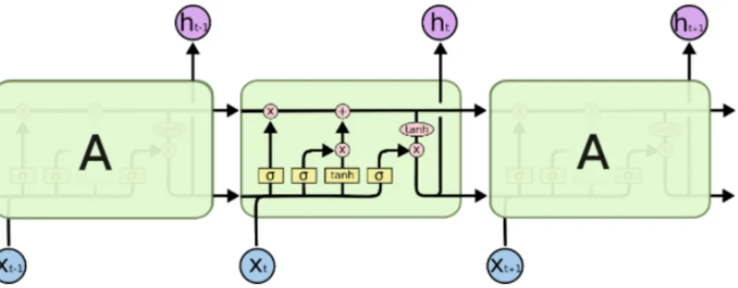
nonlin-ear activation functions usually implemented as hyperbolic tangents that squash the values in [ 1, 1]. is the entry-wise multiplication be-tween two vectors” [6]. Figure 2.4 contains a conceptual illustration of LSTM cells. For details on the functionality of each gate the reader is encouraged to refer to [6], [7], and [35].

Figure 2.4: A conceptual illustration of a network with 3 LSTM cells. Adapted from Olah [35].

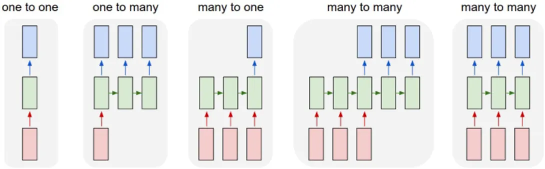
Figure 2.5: Different ways that LSTM cells can be arranged depending on what type of mapping between inputs and target is needed for the task. Adapted from Karpathy [4].

2.3 Generalization

The capacity of a neural network to fit a function to data increases as its complexity (e.g. number of hidden layers and nodes) increases. If a neural network has too much capacity for the amount of data it is given during training the network can overfit the data, i.e. learn some of the regularities pertaining to that particular set of data which may not generalize the whole population. A common sign of this is a network that performs well on training data but not on test data. There are many regularization techniques designed to remedy this in order to obtain a model that generalizes well.

2.3.1 Early stopping

Early stopping is a regularization technique that prevents a neural net-work and other machine learning models from overfitting. It is one of the most commonly used form of regularization in deep learning [36] and is often used to avoid overfitting in RNNs [37]. It works by set-ting aside part of the data used to train the model (usually denoted as the validation set) and monitoring the loss on that data (denoted as the validation loss) during training — a process often referred to as cross-validation. At first, both the training loss and validation loss decreases, but as the model starts to overfit the training loss decreases while the validation loss starts to increase. If the validation loss in-creases for some fixed number of epochs or iterations, the training is stopped and the model is chosen based on the lowest validation loss.

2.3.2 Weight decay

Weight decay is another regularization technique designed to control the complexity of a neural network by minimizing the growth of the weights in the network. This is can be done by adding a term to the error function E(w) that penalizes large weights as shown in Equation 2.8. E(w) = E0(w) + 1 2 X i w_i2, (2.8)

where is a freely tuned parameter that determines how much large weights are penalized. Krogh and Hertz [38] has shown how weight decay can improve generalization in ANNs.

2.3.3 Dropout

Dropout is a popular regularization technique for deep neural net-works presented by Srivastava et al. [39]. The technique prevents feed-forward neural networks from overfitting by randomly “dropping” a percentage of its nodes from the neural network during training. Large RNNs, unless proper regularization technique is used, also tend to overfit [40]. Zaremba et al. [40] presents a way to use dropout on LSTMs that greatly reduces overfitting on a variety of tasks including language modeling, speech recognition, image captioning, and ma-chine translation by applying it only to the non-recurrent connections in the network. “The argument for not applying it to recurrent connec-tions is that recurrence amplifies noise which in turn hurts learning” [40].

Methods

3.1 Experimental setup

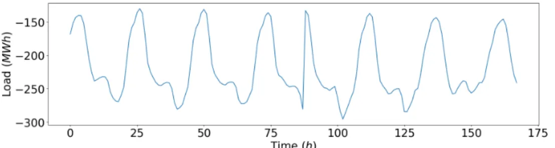
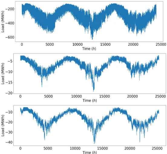
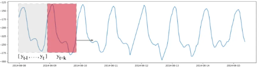
The dataset used in this project consists of electricity load and weather measurements in the form of time series for three different cities in Sweden. We denote them by set A, B, and C. Each set contains nu-merous time series with load and weather information. All datasets contain hourly measurements for 3 years, from June 2014 to June 2017. Figure 3.1 shows the load profile for the first week of dataset A. Figure 3.2 shows the entire electricity load time series.

Figure 3.1: The load profile of the electricity load time series in dataset A for the first 168 time intervals (hours). The amplitude here is the electricity load (displayed as negative power production in MWh) at any given hour t.

Figure 3.2: The electricity load time series in Datasets A (top), B (middle), and C (bottom).

3.1.1 Experiment 1

Here we design an experiment to investigate how FFNNs and LSTMs compare in day-ahead prediction. We investigate how the models’ predictive performances are affected by the length of the lookback pe-riod and sparsity of time-lagged inputs that are provided as input to the models. We also investigate how the models’ predictive perfor-mances are affected when air temperature is added as an additional feature on top of electricity load.

Two of the models, FFNN-1 and LSTM-1, receive n past observa-tions of the load, [yt l, ..., yt], where l is the length of the lookback

period. While the lookback period is varied, the length of the input vector, n, is fixed. This means that for l > n, as l is increased the

distribution of the time-lags becomes increasingly sparse. Time-lags are uniformly distributed. The output is the model’s approximation of yt+k. Input-target pairs are sampled using a sliding window approach,

as shown in Figure 3.3.

Figure 3.3: An illustration of a sliding window used to sample input-target pairs for Experiment 1. At any timestep, t, possible target values are given by yt+k. Inputs are n uniformly distributed observations [yt l, ..., yt].

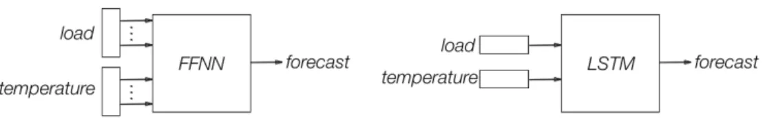
Figure 3.4 illustrates how the input vector with past observations of the load is processed by FFNN-1 and LSTM-1. The input vector can be regarded as a time-delayed input representation for FFNN-1. LSTM-1 will instead process the input vector sequentially.

Figure 3.4: A diagram illustrating how the input vector with past load is processed by FFNN-1 (left) and LSTM-1 (right).

In order to compare the FFNN and the LSTM in multivariate time series prediction air temperature data is added as extra input on top of the electricity load to both models. The air temperature time series is sampled from using the same sliding window that is used to sam-ple past observations of the load, i.e. using the same time-lags as the past observations of the load. The air temperature input vector has the same length, n, as the input load vector. Two additional models, FFNN-2 and LSTM-2, receive both past observations of the load and air temperature as input. Figure 3.5 illustrates how the input vectors are processed by FFNN-2 and LSTM-2.

Figure 3.5: A diagram illustrating how the input vectors with past load and air temperature are processed by FFNN-2 (left) and LSTM-2 (right).

Variations of the lookback period include one, two, and three days, i.e. 24, 48, and 72 hours, in order to investigate the effect of differ-ent lookback periods with increasing sparsity of time-lags on the pre-dictive performance of the models. The number of hidden nodes in FFNN-1 and FFNN-2 is fixed. The number of hidden nodes in the LSTM is adjusted such that the number of trainable parameters in both models is comparable. Table 3.1 shows the configurations of the two models and the resulting number of trainable parameters in each model1_.

Table 3.1: The number of nodes in the hidden layer of the FFNNs and the LSTMs with corresponding number of trainable parameters in each model.

Model Nodes Parameters

FFNN-1 50 1301

LSTM-1 17 1310

FFNN-2 50 2501

LSTM-2 24 2617

3.1.2 Experiment 2

Here we design an experiment that will facilitate the comparison of FFNNs and LSTMs when some restrictions of the real world are taken into consideration. We do this by adapting a configuration of a subset of input time series that were provided by Expektra. Inspired by Al-Fuhaid et al. [12] and Cheng et al. [20], we use multiple weather and and calendar variables as input to the models. However, we do not perform any feature extraction or investigate the importance of the features. Nevertheless, we believe that this might give some insight

1_{The number of trainable parameters in a model is obtained using the}

into how the models compare in a setting where the time series is a function of many other variables and as such, we might gain some insight into how the models compare when we use multiple weather and calendar variables to predict electricity load.

Table 3.2 shows a set of time series that is used as input by the benchmark FFNN in this experiment. Note how the latest observa-tions of the load have a delay of approximately 168 hours (one week) due to limitations in how soon this data is available to the system. Also note how the wind speed, humidity, solar insolation, and air temper-ature is forecasted and not observed. Apart from weather fetemper-atures a binary variable, isHoliday, indicates if the time of some observation occurs on a bank holiday, as it is also known that this has an effect on the load.

Delays are used to create time-delayed representations of a time se-ries. A positive delay d refers to the observation of that time series at time t d. The benchmark FFNN regards each input as an indepen-dent variable and predicts the electricity load at time t given inputs with delays as specified in Table 3.2. The electricity load at time t is predicted.

In order to utilize the LSTM’s ability to process data sequentially a slightly different configuration of the same input variables is proposed here. Table 3.3 shows how variables with different delays are grouped to form sequences of length 3, e.g. wind speed with delays ( 1, 0, 1). A negative delay d is mapped to the observation at time t + d. The input is then ordered chronologically. This might allow the LSTM to learn some temporal behaviour between time-delayed variables. The LSTM processes these sequences in chronological order, using a sliding win-dow of length 3 and a stepsize of 1 timestep (hour), and predicts the electricity load at time t given inputs as specified in Table 3.3.

Table 3.2: The type and name of the input variables to the FFNN with differ-ent delays.

Type Variable Delays (hours)

Observed Electricity load (target) 0

Forecasted Wind speed 0

Forecasted Humidity 0

Forecasted Solar Insolation 0

Forecasted Air temperature 0, 10, 20, 100, 200, 400, 800

Observed Electricity load 167, 168, 169

Observed isHoliday 0, 168

Table 3.3: The type and name of the input variables to the LSTM with differ-ent delays. A negative delay means using a forecasted value that is ahead of the prediction horizon.

Type Variable Delays (hours)

Observed Electricity load (target) 0

Forecasted Wind speed 1, 0, 1

Forecasted Humidity 1, 0, 1

Forecasted Solar Insolation 1, 0, 1

Forecasted Air temperature 1, 0, 1

Forecasted Air temperature 10, 20, 100

Forecasted Air temperature 200, 400, 800

Observed Electricity load 167, 168, 169

Observed isHoliday 1, 0, 1

Observed isHoliday 167, 168, 169

The number of hidden nodes is varied in the FFNN, ranging from 10 to 100. The number of hidden nodes in the LSTM is adjusted such that the number of trainable parameters in both models is comparable.

3.2 Training, validation, and evaluation

All time series are divided into three sections: the first 60% is the training set and is used for training the models. The following 20% is the validation set and is set aside for choosing model parameters

and hyper-parameters. The last 20% is the test set and is used for eval-uating the models using different error metrics. These subsets are sam-pled chronologically. Samples are not shuffled at any stage.

3.2.1 Data preprocessing

Each time series y in the dataset is scaled to the range ( 1, 1) according to Equations 3.1 and 3.2,

ystd =

y min(x)

max(y) min(y), (3.1)

yscaled = ystd⇤ (max min) + min, (3.2)

where min, max = ( 1, 1). To avoid leaking information from the test set only the training set is used to compute the statistics used for scal-ing the time series.

3.2.2 Evaluation metrics

The normalized root-mean-square error (NRMSE), given by Equation 3.3, is used to evaluate the models’ predictive performances on the test set. NRMSE = q 1 T PT t=1( ˆyt yt)2 q 1 T PT t yt2 (3.3)

3.2.3 Model optimization and regularization

Neural networks have different parameters that can be tuned to the task for the best possible performance. FFNNs can have varying num-bers of layers and numnum-bers of nodes in the hidden layers. LSTMs can have a varying number of hidden nodes in its cell. Furthermore, dif-ferent training algorithms have difdif-ferent hyper-parameters, e.g. learn-ing rate. Different methods exist for decidlearn-ing what parameters to use in order to obtain the best model. One such method is grid search where lists of parameter choices are specified for each parameter and every combination of parameters is tried. The combination of param-eters that gives the lowest validation error is picked before evaluat-ing that model usevaluat-ing the test set. The Adam [31] optimization algo-rithm is used to train the FFNNs, and the RMSprop [32] optimization

algorithm is used to train the LSTMs, and the learning rate hyper-parameters are tuned using grid search. To avoid overfitting early stopping is used to stop training if the validation error does not im-prove for 5 consecutive epochs.

3.2.4 Statistical hypothesis testing

Given different samples of NRMSE for each model and parameter con-figuration in the experiments it is useful to analyze whether the sam-ples can be regarded as coming from the same population. In the case that they do it would indicate that there is no significant difference in the predictive performance of that set of models. Different statisti-cal hypothesis tests have been designed for different situations. Those that will be useful in this project are the Kruskal-Wallis H test [41], the Friedman test [42], and Dunn’s test [43].

Results

This study consists of two main studies. The first experiment investi-gates the difference in predictive performance of FFNNs and LSTMs in day-ahead prediction. We start by testing for differences in their performance in univariate time series prediction i.e. using only past observations of electricity load to make predictions. Given that there is a limit to how many observations of past load a model can use as in-put, we also investigate whether a difference in lookback period, and consequently the sparsity of the time-lags, has any effect on the predic-tive performance of the models. Two univariate models are defined, FFNN-1 and LSTM-1, and the lookback period is one, two, and three days, using 24 evenly distributed observations in each configuration. Since many real-world problems combine time series prediction with extra inputs (e.g. [9], [10], [11], [12]) we also investigate whether there is any significant effect on the predictive performance of FFNNs and LSTMs when air temperature is added as extra input on top of elec-tricity load. Two multivariate models, FFNN-2 and LSTM-2, use air temperature as extra input in this task but still only produce load fore-casts.

The second experiment is created to facilitate the comparison be-tween FFNNs and LSTMs when practical concerns from the real world are taken into consideration e.g. availability of data to a lesser extent, or using forecasted weather factors and holiday factors on the electric-ity load. To compare the FFNN and the LSTM here we use as input to the models a subset of the variables that were provided by Expek-tra. We adhere to the restriction that the latest observation of past load is from approximately one week prior to the prediction horizon. The

optimal complexity of the network is unknown here so we vary the number of trainable parameters in both models.

4.1 Experiment 1

We started by investigating whether there were any significant dif-ferences in the predictive performance of FFNNs and LSTMs in day-ahead prediction. Four models were configured using different inputs and lookback periods as shown in Table 4.1. The key differences were the input variables used by the models, and the lookback period and sparsity of past observations.

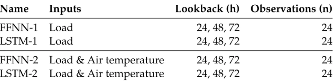
Table 4.1: The different models in experiment 1, and their differences in input and lookback. Observations refers here to the number of past observations in the input vector for some input variable. The first two rows describe the univariate models while the second two rows describe the multivariate models.

Name Inputs Lookback (h) Observations (n)

FFNN-1 Load 24, 48, 72 24

LSTM-1 Load 24, 48, 72 24

FFNN-2 Load & Air temperature 24, 48, 72 24

LSTM-2 Load & Air temperature 24, 48, 72 24

In this experiment 24 observations of past load were used since it is the minimum number of observations required to sample a full day of lookback with hourly resolution of the data. This was then fixed while the lookback period was increased to two and three days. Each model was trained and tested on datasets A, B, and C. Since random initial-ization of model weights creates some variability in the predictive per-formance this was repeated 30 times for each dataset. The NRMSEs from all three datasets were combined and grouped by model type, resulting in sets of 90 NRMSE values per model and lookback period l = (24, 48, 72).

Figures 4.1 – 4.3 contain box plots that show the distribution of NRMSEs of the different models in the different datasets. Figure 4.4 shows the distribution of the total sample population of NRMSEs of the different models.

Something that stands out in all box plots is how the range of dis-tribution of NRMSEs of LSTM-2 is often very large. In Figure 4.4 the mean RMSE of LSTM-2 can be seen to be higher than all other mod-els. It seems as though adding air temperature as extra input to the LSTM seems to have some negative effects on its predictive perfor-mance. However, to be able to draw any significant conclusions about this, as well as for the effect on using different lookbacks on the other models, or the differences in the predictive performances of the FFNN and the LSTM, we had to do some further statistical testing.

Figure 4.1: The distribution of test NRMSE values of all models on dataset A. The boxes show the range of the first and third quartile (Q1-Q3) and have a line at the median, and a diamond (⇧) marking the mean. The whiskers extend to the 5th and 95th percentile. The datapoints outside of this range (outliers) are not shown in the plots. The four models are shown in the same order as in the legend and are grouped by the lookback period. The different lookback periods are separated by the dotted vertical line.

Figure 4.2: The distribution of test NRMSE values of all models on dataset B. The box plot follows the same conventions as described in the caption of Figure 4.1.

Figure 4.3: The distribution of test NRMSE values of all models on dataset C. The box plot follows the same conventions as described in the caption of figure 4.1.

Figure 4.4: The distribution of test NRMSE values across all 90 runs of all models. The box plot follows the same conventions as described in the caption of figure 4.1.

To test whether there were any significant differences in the pre-dictive performance of the FFNNs and the LSTMs the Friedman test was conducted where the lookback period was used as the blocking factor. The test rendered a Chi-square value of 51.79 which was found to be significant (p < 0.001). In order to find which pairs of models had significantly different predictive performances we conducted post-hoc Dunn’s tests. We compared FFNN-1 with LSTM-1, and FFNN-2 with LSTM-2. We also compared FFNN-1 with FFNN-2, and LSTM-1 with LSTM-2 to investigate whether adding air temperature as extra input had any significant effect on the predictive performance of a model. Table 4.2 contains the test results from these comparisons. We found that no test result showed significant difference at the significance level ↵ = 0.05. This means that no significant difference in predictive perfor-mance was found between FFNN-1 and LSTM-1, the univariate mod-els, or between FFNN-2 and LSTM-2, the multivariate models.

Fur-thermore, adding air temperature as extra input had no significant effect on any of the two model types. Finding that adding air tem-perature as extra input had no significant effect on the LSTM seemed inconsistent with what can be seen in the box plots, which lead us to suspect possible interactions.

Table 4.2: The results from post-hoc Dunn’s test after the Friedman test for testing differences in all four models using lookback as the blocking factor. No significant difference was found between the two model types. Neither were any significant differences found between the univariate and the multivariate version of a model.

Model pair | Ri Rj | p-value

FFNN-1–LSTM-1 27.794 1.000

FFNN-2–LSTM-2 16.646 1.000

FFNN-1–FFNN-2 17.182 1.000

LSTM-1–LSTM-2 61.622 0.977

Since the Friedman test does not provide insight into possible in-teractions we decided to conduct three separate Kruskal-Wallis tests for the four models (once per lookback period). The H-statistic and p-values from these tests are shown in Table 4.3. We found that the null hypothesis was rejected for all three lookback periods (p < 0.05). Table 4.3: The results from the Kruskall-Wallis test for differences in pre-dictive performance between the four models using a certain lookback period. The hypothesis was rejected in all three tests (p < 0.05).

Lookback (h) H p-value

24 22.15 < 0.001

48 16.78 0.001

72 16.63 0.001

Post-hoc Dunn’s tests were conducted to test whether there were any differences between FFNN-1 and LSTM-1, or between FFNN-2 and LSTM-2, this time once per lookback period. The top half of Table 4.4 shows the results from these tests. We see that when the lookback period was 24 hours, the test results indicated that there were no sig-nificant difference in the predictive performance between FFNN-1 and

LSTM-1 at significance level ↵ = 0.05. Neither was there any signifi-cant difference between FFNN-2 and LSTM-2. Similarly, no signifisignifi-cant difference was found in these pairs when using 48 hours or 72 hours of lookback.

After concluding that no significant difference was found between the FFNN and the LSTM, we also conducted post-hoc Dunn’s tests to investigate whether having air temperature as extra input had any sig-nificant effect on the predictive performance of a model. That is, we compared FFNN-1 with FFNN-2, and LSTM-1 with LSTM-2. Table 4.4 shows the results from all these Dunn’s tests here. The only results that showed significant difference in predictive performance were compar-isons between LSTM-1 and LSTM-2 (p < 0.05). This correlates with what can be seen in Figures 4.1 – 4.4, and means that the LSTM showed significantly worse performance when using air temperature as extra input, compared to no extra input. Adding air temperature as extra input had no significant effect on the FFNN.

Table 4.4: The results from Dunn’s test for differences in the LSTM and the FFNN using the same inputs and a certain lookback. No significant differ-ence is found between the two model types. Only the last three rows show significant results, indicating that adding air temperature as extra input to the LSTM decreases its predictive performance.

Lookback (h) Model pair | Ri Rj | p-value

24 FFNN-1–LSTM-1 14.217 0.931 48 FFNN-1–LSTM-1 28.383 0.342 72 FFNN-1–LSTM-1 40.783 0.05 24 FFNN-2–LSTM-2 30.828 0.25 48 FFNN-2–LSTM-2 17.194 0.846 72 FFNN-2–LSTM-2 1.917 1.000 24 FFNN-1–FFNN-2 23.183 0.581 72 FFNN-1–FFNN-2 15.539 0.898 24 FFNN-1–FFNN-2 27.994 0.957 24 LSTM-1–LSTM-2 68.228 < 0.001 48 LSTM-1–LSTM-2 61.117 < 0.001 78 LSTM-1–LSTM-2 55.522 0.002

the predictive performances of the FFNNs and the LSTMs. However, adding air temperature as extra input to the LSTM was found to sig-nificantly decrease its predictive performance.

4.2 Experiment 2

In this experiment the FFNN and the LSTM were compared using multiple weather inputs, and load with a minimum time-delay of one week, as shown in Table 3.2 and Table 3.3. Two models were trained and tested on datasets A, B, and C, using different numbers of hidden nodes. Table 4.5 shows the details of the parameter configurations. Table 4.5: The parametric configurations of the FFNN and the LSTM con-sidered in this experiment with varying number of nodes in the hidden layer of each model and corresponsing number of trainable parameters.

FFNN LSTM

Parameter Hidden Trainable Hidden Trainable

Configuration Nodes Parameters Nodes Parameters

1 10 160 3 160 2 20 341 6 391 3 30 511 7 484 4 40 681 9 694 5 50 851 10 811 6 60 1021 12 1069 7 70 1191 13 1218 8 80 1361 14 1359 9 90 1531 15 1516 10 100 1701 16 1681

The models were divided into three groups of low, moderate (mid), and high complexity. The group with low complexity models was comprised of FFNNs with 10, 20, and 30 hidden nodes. The group with moderate complexity was comprised of FFNNs with 40, 50, and 60 hidden nodes. The group with high complexity models was com-prised of FFNNs with 80, 90, and 100 hidden nodes. The LSTMs were grouped similarly using the counterparts to the FFNNs. Their param-eters can be found in Table 4.5. Table 4.6 shows the mean and standard

deviation of NRMSEs of each complexity group over all datasets. Table 4.6: The mean and standard deviation (SD) of the test NRMSE of the FFNN and the LSTM grouped by model complexity.

Low complexity Mid complexity High complexity

Dataset Mean SD Mean SD Mean SD

FFNN 0.091 0.028 0.097 0.027 0.098 0.102

LSTM 0.091 0.023 0.089 0.022 089 0.021

To test whether there were any significant differences in the predic-tive performances of the FFNN and the LSTM we conducted a Fried-man test with model complexity as the blocking factor. The test ren-dered a Chi-square value of 14.14 which was found to be significant (p < 0.001). However, a post-hoc Dunn’s test showed no significant difference between the predictive performance of the FFNN and the LSTM. We ran a Friedman test using the models as the blocking factor to test for row effects on the predictive performance of the models. The test rendered a Chi-square value of 14.94 and was found to be signif-icant (p < 0.001). This lead us to conclude that there were signifsignif-icant column effects as well as significant row effects.

In spite of these likely interactions, we decided to run Kruskal-Wallis tests for differences in the FFNN and LSTM with either low, mid, or high complexity. Significant differences were found between the FFNN and the LSTM (p < 0.001). Following up with post-hoc Dunn’s tests showed that there were significant differences between the FFNN and the LSTM within all three complexity groups. Table 4.7 shows the details from this test and the post-hoc comparisons. When the complexity was low the FFNN had better performance than the LSTM. However, when the complexity was moderate or high, the FFNN had poorer performance than the LSTM. This correlates with what is can be seen in Figure 4.6, and leads us to believe that there is interaction between the model type and complexity group.

Table 4.7: Results from the Kruskall-Wallis test for differences in predic-tive performance between the FFNN and the LSTM using a certain model complexity are shown in the top half of the table. A significant difference was found between the FFNN and the LSTM in each complexity group (p < 0.05). The results from post-hoc Dunn’s tests are shown in the second half of the ta-ble. When complexity was low, the FFNN performed better than the LSTM. When complexity was moderate or high the FFNN performed worse than the LSTM. Complexity H p-value Low 13.67 < 0.001 Mid 13.06 < 0.001 High 43.5 < 0.001 Complexity | Ri Rj | p-value Low 49.652 < 0.001 Mid 48.533 < 0.001 High 88.570 < 0.001

In spite of possible interaction we decided to run Kruskall-Wallis tests for the two types of models independently, testing for differences in predictive performance when the complexity is varied. Significant differences where found between the FFNNs with different complex-ity (H = 72.17, p < 0.001) and also between the LSTMs with different complexity (H = 9.83, p = 0.007). This was followed up with post-hoc Dunn’s tests.

The results from the Dunn’s tests are shown in Table 4.8 and in-dicate that network complexity had a significant effect on both the FFNN and the LSTM. Starting with the FFNN, the results showed that there were significant differences between all three complexity groups. The FFNNs with low complexity had the best predictive performance, and as the complexity was increased the predictive performance of the FFNN decreased. This can be seen in the mean and the standard de-viation of the NRMSE of the FFNN. We can see in Figure 4.5 and Fig-ure 4.6 that the predictive performance gradually decreases as the net-work complexity is increased. In the LSTM however, the models with low complexity had significantly lower performance than the other two groups. No significant difference was found between LSTMs with moderate or high performance. This can be seen in Figure 4.5 and

Fig-ure 4.6, where the network complexity seems to have the most effect on the predictive performance of the LSTM until it reaches moderate complexity, after which the differences are no longer significant. This leads us to conclude there was indeed interaction between model type and complexity.

Table 4.8: The results from post-hoc Dunn’s test for the effect of model com-plexity on a specific type of model. The top half shows comparisons between the FFNNs with different complexity and the bottom half shows comparisons between LSTMs with different complexity.

Model Complexity pair | Ri Rj | p-value

FFNN Low–Mid 114.341 < 0.001 FFNN Low–High 167.370 < 0.001 FFNN Mid–High 53.03 0.025 LSTM Low–Mid 50.967 0.034 LSTM Low–High 57.756 0.012 LSTM Mid–High 6.789 0.982

Figure 4.5: The mean NRMSE of the FFNN and LSTM using different pa-rameter configurations as described in Table 4.5, indicated by the markers and standard deviation indicated by error bars, across all 90 runs.

(a)

(b)

(c)

Figure 4.6: The mean NRMSE of the FFNN and LSTM using different pa-rameter configurations, as described in Table 4.5. The standard deviation indicated by error bars, for dataset A (a), B (b), and C (c).

Discussion

5.1 Summary of findings

This thesis consisted of two main studies. In the first study univari-ate and multivariunivari-ate FFNNs and LSTMs were compared in day-ahead electricity load forecasting using different lookback periods. The mul-tivariate models used air temperature as extra input on top of the stan-dard electricity load, and the lookback was either one, two, or three days. We found no significant differences between the predictive per-formances of the FFNN and the LSTM. We continued to investigate whether adding air temperature as extra input had any significant ef-fect on the predictive performance of a model. We found that it had no significant effect on the FFNN. However, adding air temperature to the LSTM was found to significantly decrease the predictive performance of the LSTM.

In the second study the FFNN and the LSTM were compared using a larger number of input variables while considering restrictions that are imposed by limitations in the real world. The effect of network complexity on a network was also tested. Network complexity here refers to the number of trainable parameters (i.e. degrees of freedom) in a network. The FFNNs and the LSTMs were configured to have matching degrees of freedom. As in the first study, we found no sig-nificant difference between the predictive performances of the FFNN and the LSTM. However, we found that the predictive performance of the FFNN decreased as the network complexity increased, while the predictive performance of the LSTM increased as the network com-plexity increased.

5.2 The effect of adding air temperature as

extra input to a model

We expected that adding air temperature as extra input to a model would increase its predictive performance. However, we found that it had no significant effect on the FFNN. More surprisingly we found that it significantly decreased the predictive performance of the LSTM. These results were not congruent with previous work, e.g. Park and Mohammed [9], and Al-Fuhaid et al. [12]. However, a major difference in their work was that they used predicted future air temperature in addition to recent load and air temperature data to forecast the future load using ANNs, while we only used recent load and air temperature in our networks. While using only recent load and air temperature to predict future load is common, another approach is to learn the func-tional relationship between the load and air temperature. As in [9], the future load is then predicted using predicted air temperature informa-tion instead. It may be the case that past load did not provide much useful information to the LSTM in our study, and instead provided it with noise and decreased its predictive performance.

Despite its high correlation to the load, another aspect of the added air temperature that might support our reflection is that the added air temperature was forecasted air temperature. Perhaps using actual air temperature measurements could have had a positive effect on the predictive performance on either model. Therefore, it would be in-teresting to compare the forecasted air temperature in the datasets to actual measurements of air temperature. Residual analysis might re-veal systematic bias in the air temperature forecasts. A neural network could be trained using forecasted air temperature as input and actual air temperature as targets in order to obtain “adjusted” forecasts which in turn could be used in either the FFNN or the LSTM to make elec-tricity load predictions.

Another way to make better use of weather information for pre-dicting electricity load might be to separate the weather sensitive com-ponents from the load before learning the relationship between the weather information and those components. Seeing that there are reg-ularities such as the seasonal cycles that depend mostly on the time of the day, week, or year, extracting those from the load first might reduce some of the information that could prevent the network from learning

any meaningful relationship between air temperature and load. An in-teresting approach to this was proposed by Chen et al. [10], who used a non-fully connected FFNN in electricity load forecasting. Seeing that the load is a nonlinear function of multiple variables, they aimed to first extract, and then approximate this nonlinearity. In their net-work there were multiple supporting netnet-works. One netnet-work formed a connection between the current load and the output, while another formed a connection between air temperature inputs and the output, etc. They argued that this approach improves the learning efficiency and model accuracy.

5.3 The effect of different lookback periods

Zheng et al. [21] showed that the LSTM outperformed the FFNN in electric load forecasting. In their study however, a much longer look-back, 10 days, was used to forecast electricity load the next day. Zheng et al. [21] argued that it is important to consider the long term depen-dencies in time series prediction. They argued that the FFNN has in-sufficient capability of modeling long term dependencies due to mak-ing the independence assumption about the load observations. Since the LSTM does not make this assumption it is presented as a better alternative and may explain why the LSTM outperformed the FFNN in their experiments. However, in our experiments the lookback may not have been long enough for the LSTM to learn such long term de-pendencies. It might also be that the number of time-delayed vari-ables were not large enough to motivate a sequential approach, which would explain why the LSTM did not outperform the FFNN in our study. The limitations that this poses to the LSTM is discussed briefly in Section 5.5.

In spite of this, it is still interesting that we find the predictive per-formances of the FFNN and the LSTM to be comparable as we increase the lookback from one to two, and even to three, days. The past obser-vations become increasingly sparse, yet the predictive performances of the two models remain comparable. This suggests that none of the two model types is particularly better at electricity load forecasting us-ing data of lower than hourly resolution. A practical concern related to this is handling gaps in time series data. The FFNN handles gaps suc-cessfully by viewing time-delayed variables as independent, whereas

gaps in a sequence could be seen as discontinuities. However, our findings suggest that the LSTM is not affected negatively by increas-ingly sparse time-delays, anymore than the FFNN. This could be in-vestigated further by testing the effect that the resolution of the input data has on the predictive performance of the two types of models in-dependently. In order to gain even more insight into this, it would be interesting to artificially create unexpected gaps in the data as opposed to regular gaps that are a result of lower resolution of the data. The predictive performance of a model that uses continuous data could be compared to that of a model that receives data with unexpected dis-continuities. These findings would give further insight into whether any of the two types of models handle unexpected gaps in the data differently. The implication of a model that can learn long time depen-dencies in time series data and successfully handle gaps in the data, or data of lower resolution, would be the possibility to reduce over-head. Reducing overhead by lowering the compute time required to process large amounts of data results in cost reductions for a company. The computational resources could be spent on further improving the models.

5.4 The effect of network complexity on

pre-dictive performance

Testing whether network complexity had any significant effect on the models independently, we found that the best option for the FFNN was low complexity and that its predictive performance gradually de-creased as the complexity grew. The LSTM showed different behaviour, where the predictive performance was worse when the complexity was low, while it was better for moderate and high complexity. How-ever, no significant difference was found between using moderate and high complexity in the LSTM. This suggests that the LSTM requires a larger number of parameters to perform well in time series prediction. This translates into requiring more compute time, which is a finite and valuable resource. Therefore this is worth to take into consideration when deciding whether to use the LSTM in electricity load forecast-ing.

5.5 Limitations

These findings do not strongly motivate the use of LSTMs for nonsta-tionary time series prediction. However, the thesis was limited to time series prediction using a relatively small number of past observations and short period of lookback as input to the models. In problem do-mains where the expected maximum extent of time dependencies is not larger than what was used here the advantages of the gated recur-rent connections in the LSTM may not be fully utilized. LSTMs have been demonstrated to be useful in other domains where the sequences are longer (e.g. character level language modelling with sequences of 100 characters [4]). Therefore, it may have been more interesting to investigate whether the LSTM is able to learn any long-term depen-dencies in the time series data.

5.6 Ethics and sustainability

In the European Union (EU) the Renewable Energy Directive1

estab-lishes a policy for the production and promotion of energy from re-newable sources and requires the EU to fulfill at least 20% of its total energy needs with renewable energy by 2020.

This thesis contributes to the improvement of electricity load fore-casting. Improved load forecasting allows for optimal matching of en-ergy supply and demand which results in higher penetration of re-newable power into our energy systems. This reduces the amount of carbon emissions into the atmosphere which in turn has a positive ef-fect on the environment.

Improved load forecasting also improves operational planning of electrical utilities. Reducing the risk for over- or under-contracting and then selling or buying power on the balancing market can lead to lower costs for consumers at a societal level, and even save a util-ity from bankruptcy at the corporate level [44]. Reducing these costs allows us to spend resources on further improvements of our energy systems or other operations that aim to make our cities more sustain-able and reduce their negative impact on the environment.

1

Conclusion

In this thesis the predictive capabilities of FFNNs and LSTMs were compared in the problem of electricity load forecasting. We did not find any conclusive evidence in favour of LSTMs, as originally hy-pothesized. However, some key differences were found between the two neural network approaches.

In the first study the FFNN and the LSTM were compared in day-ahead electricity load forecasting using a lookback period of either one, two, or three days. Both univariate and multivariate configu-rations of the models were considered, where the univariate models used only past electricity load, while the multivariate models used past load and air temperature, to make predictions. Adding air tem-perature as extra input to the FFNN had no significant effect on its predictive performance. However, adding extra air temperature in-formation to the LSTM significantly decreased its performance, which reflected suboptimal handling of multivariate time series data.

In the second study the FFNN and the LSTM used a larger number of inputs to predict electricity load. Furthermore, the most recent ob-servation of the electricity load was one week prior to the prediction horizon. The networks were also configured to have either a low, mod-erate, or high number of trainable parameters, here referred to as the network’s complexity. No significant difference was found between the predictive performance of the FFNN and the LSTM. However, we found that as we increased the complexity of the FFNN its predictive performance decreased significantly, while increasing the complexity of the LSTM increased its predictive performance.

We believe that the input sequences were too short for the LSTM to

effectively learn time dependencies in the load data. This was a limi-tation for the LSTM models, and in the thesis overall, and should have been considered when designing the experiments in this thesis. In con-clusion, no significant differences were found between the predictive performances of FFNNs and LSTMs. Thus, we cannot give recommen-dations for using the LSTM in electricity load forecasting. This work serves as a useful reference for the researcher and the industry in mak-ing an informed decision about whether to use the LSTM in electricity load forecasting.

6.1 Future work

LSTM networks have a capability of storing information for very long periods of time [6]. Therefore, one possibility for future investigations would be increasing the number of observations in the input vector. Another idea is to use unevenly distributed and increasingly sparse time-delays (e.g. logarithmically spaced time-delays) as input to the LSTM. It would be very interesting to see whether this has any effect on the predictive performance of the LSTM in electricity load forecast-ing.

Another test that would be interesting for time series prediction is the use of LSTMs for automatic feature extraction. Laptev et al. [45] explored the possibility of having “a single generic neural network model capable of producing high quality forecasts for heterogeneous time series relative to specialized classical time series models”. It could also be an opportunity for future studies.

[1] H. K. Alfares and M. Nazeeruddin, “Electric load forecasting: Literature survey and classification of methods”, International journal of systems science, vol. 33, no. 1, pp. 23–34, 2002.

[2] F. Virili and B. Freisleben, “Nonstationarity and data preprocess-ing for neural network predictions of an economic time series”, in Neural Networks, 2000. IJCNN 2000, Proceedings of the IEEE-INNS-ENNS International Joint Conference on, IEEE, vol. 5, 2000, pp. 129–134.

[3] R. S. Tsay, “Outliers, level shifts, and variance changes in time series”, Journal of forecasting, vol. 7, no. 1, pp. 1–20, 1988.

[4] A. Karpathy, “The unreasonable effectiveness of recurrent neu-ral networks”, Andrej Karpathy blog, 2015.

[5] J. T. Connor, R. D. Martin, and L. E. Atlas, “Recurrent neural networks and robust time series prediction”, IEEE transactions on neural networks, vol. 5, no. 2, pp. 240–254, 1994.

[6] F. M. Bianchi, E. Maiorino, M. C. Kampffmeyer, A. Rizzi, and R. Jenssen, “An overview and comparative analysis of recurrent neural networks for short term load forecasting”, arXiv preprint arXiv:1705.04378, 2017.

[7] S. Hochreiter and J. Schmidhuber, “Long short-term memory”, Neural computation, vol. 9, no. 8, pp. 1735–1780, 1997.

[8] K. Cho, B. Van Merriënboer, C. Gulcehre, D. Bahdanau, F. Bougares, H. Schwenk, and Y. Bengio, “Learning phrase representations using rnn encoder-decoder for statistical machine translation”, arXiv preprint arXiv:1406.1078, 2014.

[9] D. C. Park and O. Mohammed, “Artificial neural network based electric peak load forecasting”, in Southeastcon’91., IEEE Proceed-ings of, IEEE, 1991, pp. 225–228.

[10] S.-T. Chen, D. C. Yu, and A. R. Moghaddamjo, “Weather sensi-tive short-term load forecasting using nonfully connected artifi-cial neural network”, IEEE Transactions on Power Systems, vol. 7, no. 3, pp. 1098–1105, 1992.

[11] C. Chen, Y. Tzeng, and J. Hwang, “The application of artificial neural networks to substation load forecasting”, Electric Power Systems Research, vol. 38, no. 2, pp. 153–160, 1996.

[12] A. S. Al-Fuhaid, M. A. El-Sayed, and M. S. Mahmoud, “Neuro-short-term load forecast of the power system in kuwait”, Applied Mathematical Modelling, vol. 21, no. 4, pp. 215–219, 1997.

[13] D. C. Park, M. El-Sharkawi, R. Marks, L. Atlas, and M. Damborg, “Electric load forecasting using an artificial neural network”, IEEE transactions on Power Systems, vol. 6, no. 2, pp. 442–449, 1991. [14] K. Lee, Y. Cha, and J. Park, “Short-term load forecasting using

an artificial neural network”, IEEE Transactions on Power Systems, vol. 7, no. 1, pp. 124–132, 1992.

[15] R. Mbuvha, “Bayesian neural networks for short term wind power forecasting”, Master’s thesis, KTH, School of Computer Science and Communication (CSC), 2017, p. 48.

[16] L. Åkerberg, “Using unsupervised machine learning for outlier detection in data to improve wind power production predic-tion”, Master’s thesis, KTH, School of Computer Science and Communication (CSC), 2017.

[17] D. Srinivasan and M. Lee, “Survey of hybrid fuzzy neural ap-proaches to electric load forecasting”, in Systems, Man and Cyber-netics, 1995. Intelligent Systems for the 21st Century., IEEE Interna-tional Conference on, IEEE, vol. 5, 1995, pp. 4004–4008.

[18] P. Mandal, T. Senjyu, N. Urasaki, and T. Funabashi, “A neu-ral network based seveneu-ral-hour-ahead electric load forecasting using similar days approach”, International Journal of Electrical Power & Energy Systems, vol. 28, no. 6, pp. 367–373, 2006.

[19] D. L. Marino, K. Amarasinghe, and M. Manic, “Building energy load forecasting using deep neural networks”, in Industrial Elec-tronics Society, IECON 2016-42nd Annual Conference of the IEEE, IEEE, 2016, pp. 7046–7051.