Returns to Education
in Germany:
MASTER
THESIS WITHIN: Economics NUMBER OF CREDITS: 30
PROGRAMME OF STUDY: Economic Analysis
AUTHOR: Cláudio Correia Rosa JÖNKÖPING May 2021
An updated assessment of the earnings-education
relationship
Master Thesis in Economics
Title: Returns to Education in Germany: An updated assessment of the earning-education relationship
Authors: Cláudio Correia Rosa Tutor: Andreas Stephan
Date: 2021-05-24
Key terms: Returns to education; Mincer Equation; Germany; Human Capital
Abstract
This work aims at answering the following questions: what is the gain in future earnings from spending one more year in schooling? Do all years in education increase one’s wages by the same amount? Will obtaining a diploma positively affect one’s future wage? By running a Mincer equation enhanced with factors such as sector of employment or gender and using the educational attainment of the parents as an instrumental variable on the 2017 wave of the German Socio-economic Panel, I am able to estimate that in Germany, returns to education are around 10%. To circumvent endogeneity and omitted variable bias, 2SLS is favoured against OLS. Despite this, the results are similar to previous literature which employed a simple OLS on a Mincer equation though it is also found that OLS underestimates returns to education by 1.2%. Returns to the school years themselves are estimated to be more or less stable and fluctuate between 6 and 12% with the exception of the 9th year of schooling which is more impactful at 24% and the 14th at zero. Finally, due to the complex nature of the German educational system, it was not possible to ascertain the existence of diploma effects.
Table of Contents
1.
Introduction ... 1
1.2 The German Education System ... 3
2.
Literature Review ... 4
2.1 An Overview... 4
2.2 Why there is a relationship between education and income ... 9
2.2.1 The Human Capital Hypothesis ... 9
2.2.2 The Screening (or Signalling) Hypothesis and its opposition to and by the human capital theory. ... 9
2.3 Calculating the returns to education. ... 12
2.3.1 Measuring Earnings ... 12 2.2.2. Measuring Education ... 12 2.2.3. Measuring Ability ... 15 2.3.4 Assorted Variables ... 17 2.3.5 Instrumental Variables ... 18
3.
Methodology... 20
4.
Data ... 21
5.
Results and Discussion ... 26
5.1 Returns to Education ... 26
5.2 Screening or Human Capital ... 31
6.
Conclusion ... 33
7.
Reference list ... 35
1. Introduction
Education is a period that most, if not everyone, goes through. Thus, at some point all must make the choice to leave it. Here is where the returns to education become relevant: what is the gain in future earnings from studying one more year? Do all years in education increase one’s wages by the same amount? Will obtaining a diploma positively affect one’s future wage? These are questions that an individual might pose themselves when considering leaving their academic life, and questions this thesis aims to discuss. For that purpose, it employs a sample from Germany from 2017—the German Socio-economic panel (SOEP). This sample includes the academic choice of thousands of individuals, their earnings as well as other specificities (the sector in which they are employed, for instance) to enhance the accuracy of the results. Using the year 2017 allows for an analysis that is not out of date whilst, at the same time, all the required variables are present.
In theory, a person would only continue studying if returns to education are high enough to justify them not joining the labour market. Indeed, some researchers see studying as any other type of investment (say a capital investment) and compare rates of return between these choices (see for instance, Psacharopoulos, (1972, 1985, 1994, 2004)). This is because the opportunity cost of joining the labour force is always present: one may start earning money today by leaving schooling at the cost of increased future earnings, if this increase is not high enough (Spence, 1973; Lemieux, 2003).
To make this choice one should also consider the pattern of returns to schooling, should they not be linear. Psacharopoulos (1987) and Frazis (2002) argue that just like with physical capital, human capital should have decreasing returns to productivity and this would be seen by decreasing returns on wages. On the other hand, some research (Hungerford & Solon, (1987), Mora (2003), to name a few) found higher returns to school years which, when completed, award a student with a diploma. This phenomenon is referred to as the sheepskin effect, the diploma effect and credentialism: whereby, returns to schooling come mainly from one’s attainment of a certificate (Hungerford & Solon, 1987).
Furthermore, the last research question introduces an interesting discussion regarding the earnings-education relationship. Namely, the source of returns to education: thus, this work also contributes to the problematisation of human capital versus screening. Whilst in the end it was not possible to conduct an empirical analysis of the two hypotheses due to the sample for a required variable being too small, the discussion is nonetheless provided on the comparison of the two theories and how they would apply in a German context. The German education system is also ideal for such an analysis as having academic tracks of different durations allows for the comparison of different-track students subject to the same labour market conditions.
Education is also an important variable from a macroeconomic perspective. It is a crucial variable in neo-classical growth models, (see for instance Solow (1956) Lucas (1988), Romer (1990), Mankiw, Romer, & Weil (1992)). In these models, education is part of what the authors call human capital. The above models see human capital as an element that enhances the production function thus making labour and capital more productive. Sianesi & van Reenen (2003) analysed the effects of an increase in the level of education1 of the population on economic growth (and/or growth rate). Their analysis applies both neo-classical models; which found that increasing the education level resulted in an increase of output per capita by three to six percent, and new-growth theories; whose conclusion is that the growth rate would increase by around one percent. Further, they find that the education level impacts economic growth at different rates: tertiary being the most beneficial towards GDP growth (Sianesi & Van Reenen, 2003). An explanation for this growth can be that there are social returns to education: Canton (2007) finds that an increase in the educational level leads to a raised labour productivity by a factor of seven to ten percent in the short-run or eleven to fifteen in the long-run.
There is also the discussion on the civic returns to education. That is, externalities to one’s academic life. Dee (2004) found evidence of the more educated to also be more politically active (as measured by voting participation) and more likely to be in favour of free speech. Furthermore, the author used newspaper readership as a proxy for political involvement, claiming that those who read newspapers are better informed on current topics, and found
1 Measured as either years of schooling or percentage of people who obtained the degree in question
a positive relationship between that and education (Dee, 2004). Long (2010) agrees with Dee (2004) as he also founds a higher voting participation in those who are more educated. Beyond that, Long (2010) concluded there is a negative relationship between education and divorce rates, having children and an early marriage.
Finally, one of the challenges of calculating returns to schooling is the issues of endogeneity and omitted variable bias. To tackle these, a 2SLS model is favoured instead of OLS whereby the instrumental variables to predict education are the educational attainment of the mother and the father of the individual. This may have the limitation that if ability is transferred from one’s parents, even the predicted value will be correlated with ability which would not solve the omitted variable bias.
1.2 The German Education System
As mentioned, this thesis is an analysis of returns to education in Germany, unlike the American and other European education systems, the German one is less linear. This means students’ paths through their academic life branch off earlier than what is common in other countries. To further complicate this, since each state has control over its educational system, there are intra-country differences in the academic system. Regardless, school begins at age 6 with primary school (Grundschule) which lasts four years2. After that, students begin secondary school which is divided into three different curricula. The basic track (Hauptschule) is usually taken by students who will enrol in an apprenticeship when their education is over. This track lasts for five years (may vary according to state). Then there is the middle track (Realschule) which is “more academically rigorous” than the Hauptschule. This lasts six years and students will move on to an apprenticeship or vocational studies. Finally, and the most academically demanding is the Gymnasium. This lasts around ten years if the student intends to attend a university or nine if they prefer a polytechnic. Compulsory schooling is nine years in the Gymnasium and ten years in the other tracks. Following that, begins tertiary education which includes universities, polytechnics, and other German institutions. Considering which track a student was assigned to can be an important predictor of income since there is a hierarchy of academic rigor between the three tracks (Ammermüller & Weber, 2005). (Studying in Germany, 2021)’ (Pischke & von Wachter, 2005)
2. Literature Review
This section has three objectives. Firstly, it aims at giving an overview of past literature that ascertained the returns to education in diverse countries. The reason for which it does not focus on one type of country (say developed/developing) is to show what differences in returns there are in different countries. Secondly, it intends to show how the returns to education are calculated: what variables are used and what are their alternatives. Finally, it endeavours to explain why there is a relationship between increased earnings and education.
2.1 An Overview
One of the first contributors to the calculation of the returns to education across countries is Psacharopoulos. He starts in 1972 estimating the benefit to attaining an education, dividing the school years into primary, secondary and tertiary. He obtains his results by using averages. He divides the average cost of a level of education (say university or tertiary degree) by the expected average annual increase in earnings. He also distinguishes between a private and a social rate of return. The former takes the perspective of the individual: considering only what the student pays and what they get in return. The latter, however, expands the definition to include external costs and benefits such that it is more useful for policy makers rather than student-candidates. The author, nevertheless, admits that this assumes that the benefits are perpetual. In his table which compiles his results for several countries’ results in the 60’s, we can see that the returns to education were at least 8% for primary school in the Philippines and as high as 66% for primary school in Uganda. What Psacharopoulos finds is that private returns are higher than the social ones (possibly explained by the fact that education is government-subsidised, therefore, it is not the individual who bares them) where for instance, private returns to primary school in the USA were 155% whilst only 17,8% for social returns; for most countries, the returns to education decrease with a higher education level, such that primary education yields the highest returns and tertiary the lowest (relative to the previous level that is); developing countries show higher returns to education; and finally, these rates of return are higher than the rates for other investment opportunities. (Psacharopoulos, 1972)
Psacharopoulos updates his study in 1985. Returns to education are still the highest for primary education and in developing countries: in Asia, the private returns for primary school were 31% whilst for secondary education were 15%. The author explains that primary education yields the highest returns because it is the cheapest education level and the difference in productivity between those who cannot read or write and those who have attained this skill is the highest among all other levels. Psacharopoulos also finds the there is a negative relationship between country per-capita income and the rate-of-return to schooling. He explains this difference is due to a lower proportion of human-to-physical capital in developing countries which makes skilled labour more valuable. Indeed, this difference can also be found in Europe in the 70s and 80s (Harmon, Oosterbeek, & Walker, 2003). The 1985 update also uses a new method of calculating the returns whereby one would employ the Mincer equation: a regression of the years of schooling, experience and experience squared on the logged earnings. This method would become a common way of calculating returns (indeed, see table 1 for a list of literature that applies it). The author updates his calculations in 1994 and again in 2004. His findings hold for other studies as well, both dates and Psacharopoulos re-affirms the human capital theory (expanded below) to explain why returns to education exist. (Psacharopoulos, 1985), (Psacharopoulos, 1994), (Psacharopoulos & Patrinos, 2004)
More recent studies, however, do show increased returns for later academic phases. In Spain, returns to education increase by around 30% after high school (Alba-Ramírez & San Segundo, 1995). Asadullah (2006) compiles data for several South-East Asian countries and finds that higher education awards returns to schooling that are higher than all the previous education levels (except for Nepal). In India, they were found to increase until the university level which shows lower returns (Duraisamy, 2002). The reason for this change might be that labour has become more specialised and thus employers need and financially reward highly educated workers.
Using this information, the table below shows examples of studies which have calculated the returns to education in several countries. This table includes a variety of countries and different time periods.
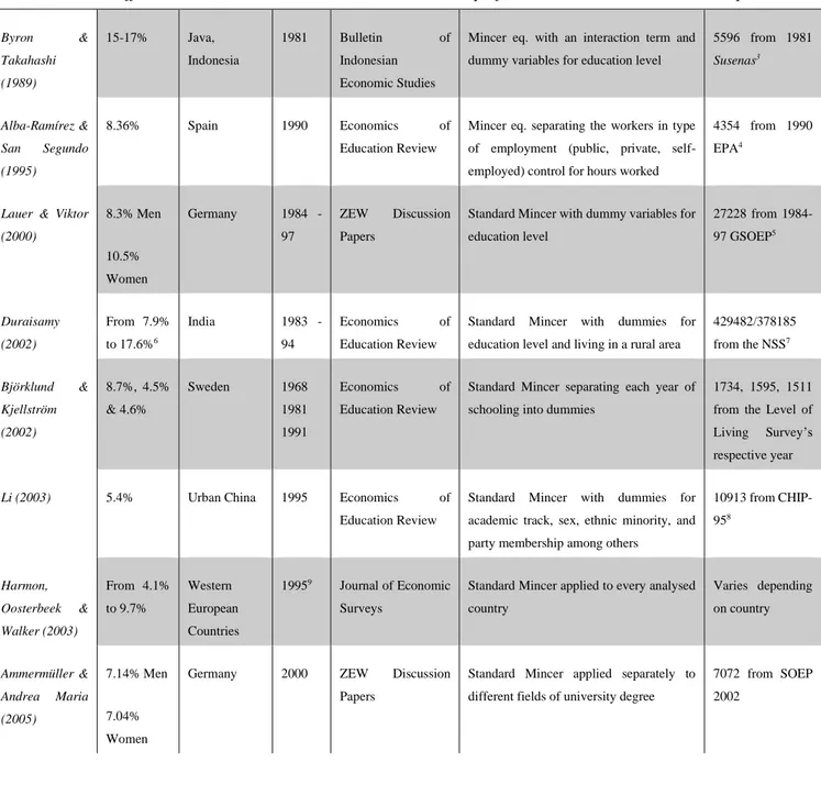
Table 1: Compilation of studies on returns to education
Article Coefficient Location Year Journal Specificities Sample size
Byron & Takahashi (1989) 15-17% Java, Indonesia 1981 Bulletin of Indonesian Economic Studies
Mincer eq. with an interaction term and dummy variables for education level
5596 from 1981 Susenas3 Alba-Ramírez & San Segundo (1995) 8.36% Spain 1990 Economics of Education Review
Mincer eq. separating the workers in type of employment (public, private, self-employed) control for hours worked
4354 from 1990 EPA4
Lauer & Viktor (2000) 8.3% Men 10.5% Women Germany 1984 -97 ZEW Discussion Papers
Standard Mincer with dummy variables for education level 27228 from 1984-97 GSOEP5 Duraisamy (2002) From 7.9% to 17.6%6 India 1983 -94 Economics of Education Review
Standard Mincer with dummies for education level and living in a rural area
429482/378185 from the NSS7 Björklund & Kjellström (2002) 8.7%, 4.5% & 4.6% Sweden 1968 1981 1991 Economics of Education Review
Standard Mincer separating each year of schooling into dummies
1734, 1595, 1511 from the Level of Living Survey’s respective year
Li (2003) 5.4% Urban China 1995 Economics of Education Review
Standard Mincer with dummies for academic track, sex, ethnic minority, and party membership among others
10913 from CHIP-958 Harmon, Oosterbeek & Walker (2003) From 4.1% to 9.7% Western European Countries 19959 Journal of Economic Surveys
Standard Mincer applied to every analysed country Varies depending on country Ammermüller & Andrea Maria (2005) 7.14% Men 7.04% Women
Germany 2000 ZEW Discussion
Papers
Standard Mincer applied separately to different fields of university degree
7072 from SOEP 2002
3 National Socio-Economic Survey for Indonesia 4 Labour Force Survey
5 German Socio-Economic Panel
6 Primary: 7.9%; Middle 7.4%; 17.3% Secondary; Higher secondary 9.3%; College/University 11.7%;
Technical diploma/certificate 14.6%
7 National Sample Survey
8 Chinese Household Income Project
Pischke & Wachter (2005) 7.2% or 0.7%10 Germany 1980 - 1990 NBER Working Paper Series
Standard Mincer as well as a dummy for if the State had changed its mandatory Schooling laws 5412611 and 75041612 Asadullah (2006) 7% Bangladesh 1999 to 2000 Education Economics
Standard Mincer with dummies for rural area, religious minority and landholding
5668 from HIES13
1999-2000
Aakvik, Salvanes & Vaage (2010)
8.2% Norway 1995 European Economic
Review
Ordered Probit model 203387 from
Statistics Norway 1995 Barouni & Broecke (2014) Ranges from 2%-73%14 12 African Countries 2005 to 201115 Journal of Development Studies
Several methods, including Mincer, short-cut and elaborate/full method
Diverse household surveys Bhuller, Mogstad & Salvanes (2014) 10.5%-14% Norway 1967 to 2010 NBER Working Paper Series
Standard Mincer with IV for an educational reform 600679 from Statistics Norway 1967-2010 Kamhöfer & Schmitz (2016)
0% Germany 2006 Journal of Applied
Econometrics
Standard Mincer augmented with number of schools per 1000km2 and exposure to an
educational reform
5500 from 2006 SOEP
The majority of the studies in the table applied the Mincer equation or an enhanced version of it. The only exception is Aakvik, Salvanes, & Vaage (2010) who employ a probit model. By employing a Mincer equation, researchers have to find a measure of education and ability. The most common measure of education in the above collection was years of schooling, however, facing data limitations, Aakvik, Salvanes, & Vaage (2010) employ a dummy variable for the level of education (primary, secondary, etc). The most common measure of ability was expected labour market experience or age. One should, however, when comparing the results of the above papers, remember that the studies were performed in different time periods which may explain some of the discrepancies. Having that in mind, developing countries (India, Indonesia and the African countries in Barouni & Broecke (2014)) show higher returns than the studies on developed countries (Duraisamy, 2002), (Byron & Takahashi, 1989). The exception is
10 When using an increase in the age from dropping out, instead of the years of schooling, the rate of return
drops to close to zero.
11 Qualifications and Career survey (1979, 1985-86, 1991-92 and1998-99) 12 Micro-census (Waves from 1989, 1991, 1993 and from 1995 to 2001) 13 Household Income Expenditure Surveys
14 Numbers correspond to Upper secondary schooling. The article also shows that for basic school the range
is between 1%-8% and 10%-50% for Tertiary education, using a Mincer Model.
Asadullah (2006) which found 7% returns to education in Bangladesh: an amount comparable to what was found in the studies on European countries (for instance, Harmon, Oosterbeek, & Walker (2003)).
Perhaps the most striking papers in the table, and the most relevant too, are those that found close to zero returns to education in Germany. Pischke & von Wachter (2005) study whether an education reform had an effect on the returns to education. This reform concerns an expansion of compulsory schooling to include a 9th year. They apply a slightly different model to their two samples. Firstly, they use a quartic function (instead of linear or quadratic) experience (measured either as potential experience in the labour market or age). In their most basic model (which includes only controls for experience, gender and state) they find that the returns to education are between 7.2% and 8.3% for the QaC and the Micro Census, respectively. Using age instead of potential experience leads their estimates to drop to 6.1% and 7.4%. What is most notable is when a dummy for whether the state had introduced the aforementioned reform replaces the variable for years of schooling, the returns to education turn to zero and remain very small (1.9% and 0.5%) even when adjusting for state specific trends. Kamhöfer & Schmitz (2016) replicate Pischke & von Wachter’s (2005) study and reach the same conclusion. Comparing it to two studies that found positive returns to education (Lauer & Steiner, (2000) and Ammermüller & Weber, (2005)) the biggest difference is the variable for schooling. The studies which show zero returns, control for the expansion of mandatory schooling instead of years spent in education. One could criticise these articles for using a measure that gives odd or counterintuitive results, however, employing the same variable for schooling in other countries has showed positive returns. Oreopoulos (2003), for example, analysed a similar reform in the Canadian, British and American educational systems and he found positive returns to education (from 7.4 to 14%). These are higher in Canada than in the US or the UK: the latter of which shows the lowest returns with only 7.4%. Another article which analysed the impact of an educational reform on schooling is Acemoglu & Angrist (2000) which when performing a similar analysis on the US found returns from 6.3 to 11.3% depending on which birth cohort and instruments used.
The other studies present in table 1 are mentioned throughout the text as their relevance surges.
2.2 Why there is a relationship between education and income
Having shown all the studies pointing at the existence of a relationship between schooling and earnings, it is interesting to ponder why this association exists. Researchers point to several theories explaining why the more educated earn more. The human capital theory and the screening theory are the most cited.
2.2.1 The Human Capital Hypothesis
This theory was started formulated by Becker (1962). In his article, he sees education completely as an investment which entails costs and returns. The costs to education can be the university fees but also the foregone wages of working instead of studying. A return in this sense would be the increase of the worker/student’s future wage. Thus, from the author’s perspective, one’s salary increases because of one’s ability (one’s human capital). The latter, in turn, is gained or accumulated by spending time in schooling, training, etc (Becker, 1964, 1975, 1983). Thus, following this train of thought, the relationship between earnings and education comes from the enhanced productivity of the more educated. Psacharopoulos (1987) names a few details to validate the human capital theory. For instance, if this theory is correct, there would be diminishing returns to education as there are with physical capital. This is observed by the author whose findings support the human capital theory. Despite the author finding diminishing return to education, he defends that these are still high enough to justify further education expansion.
2.2.2 The Screening (or Signalling) Hypothesis and its opposition to and by the human capital theory.
The screening theory was kickstarted by Spence (1973) who, in his article, describes the hiring process through the lenses of an employer. Initially, the employer does not know how productive a candidate is. This employer will, instead, hire their workers based on their characteristics. These can be either fixed or alterable. Those that can be altered are referred to as “signals” by Spence. In turn, candidates can invest in signals by paying the signalling cost. Theoretically, they will do this only if the benefit is greater than the cost. Perhaps ironically, if the latter applies, every candidate would acquire that signal making
them indistinguishable. Thus, Spence assumes that signalling costs and productivity are negatively correlated. That is, signalling costs are higher for those with less productive capabilities. Under these assumptions, equilibrium is only reached after several hiring cycles where employers’ expectations solidify giving an advantage to those that can acquire signals more cheaply which in turn would be more productive in Spence’s model. (Spence, 1973)
It is, thus, complicated to prove signalling theory, since one of its characteristics is that workers’ ability is hidden from employers but also from researchers (Frazis, 2002). Despite this, Spence’s signalling theory has been applied in several fields (like Psychology or Anthropology) to analyse a myriad of signals jobseekers use to indicate their ability (Karasek & Bryant, 2012).
The way Layard & Psacharopoulos (1974) explain this theory is that education serves as a filter through which only those with pre-existing abilities can pass. Consequently, this implies that education does not, on its own, improve one’s productivity. The authors, however, cast doubt on the validity of this theory as they find that their returns to education are the same between those who completed their education and those who dropped out. Secondly, Layard & Psacharopoulos (1974) explain that, as employers obtain more information about a worker’s ability, education should play a lesser role on their earnings (thus decreasing the returns to education for older employees). Despite this, the authors find the exact opposite: older employees’ returns to education are higher than the younger ones’. Finally, if the objective of education is to screen those with pre-existing abilities, there would be cheaper ways of doing so (Layard & Psacharopoulos, 1974).
On the other hand, Hungerford & Solon (1984) write about the sheepskin effect on the returns to education and criticise Layard & Psacharopoulos (1974) for being too hasty in dismissing the screening hypothesis. The sheepskin effect consists in, as mentioned, higher returns to education for those who have a degree relative to those who do not (keeping all else equal). These is also referred to as the diploma effect. As opposed to Layard & Psacharopoulos (1974), Hungerford & Solon (1984) do find a significant sheepskin effect. The discrepancy can lie on the different specification and sample. Whilst Hungerford & Solon (1984) affirm that rejecting the screening hypothesis was premature for Layard & Psacharopoulos (1974), they, in turn, recognise that there can be
explanations other than the screening theory. Namely, Chiswik (1973) who writes that one of the reasons students drop out of school is that they do not see education improving their ability. The students who remain in school feel the opposite: the education system enhances their productivity, so they opt not to drop out (Chiswik, 1973). Chiswik (1973), in a way, bridges the gap between the two theories: education improves the ability of some students who, in turn decide to remain in education, whilst not enhancing other pupils’ capabilities.
One of the issues that several researchers ascertained (see for instance Frazis (2002), Park (1994)) is the irregular pattern of returns to education throughout one’s years of schooling. For example, a student, in the US, obtains a college degree at sixteen years of schooling; those who drop out of their degree, however, have between thirteen and fifteen years, instead; if the human capital hypothesis applies, someone who studied for fifteen years would have acquired some level of human capital similar to sixteen years sooner than thirteen. Despite this, when Frazis (2002) estimates the returns to education on the American Current Population Survey of 1977-1991 (calculating the returns to education for every year individually), he finds that those who drop out at fifteen years of schooling have slightly lower returns than those with fourteen. His other findings show that years twelve and sixteen show the highest jump returns (15.1 and 22.0% respectively). These are the years an American student earns their high school and first university diploma, respectively. Another interesting result is the higher-than-expected (9.9%) returns of those with thirteen years of schooling (those who drop out in their first year at the university). Frazis (2002) mentions this is due to a “college entrance effect” whereby someone who was admitted into college enjoys higher earnings, despite not completing their education.
Park (1994) analyses the anomaly of the fifteenth year on different regards: personal & employment characteristics, whereby people who study for exactly fifteen years tend to choose jobs which are prone to lower pay; dropouts at fifteen may have experience curves which are flatter than others; the fifteenth year may be less relevant for someone’s education; signalling theory and sheepskin effects. According to him, the best explanation is the measurement error whereby people who claim to have fifteen years of schooling actually have fourteen and answer to the questionnaires erroneously (Park, 1994).
2.3 Calculating the returns to education.
Having given an overview of the topic, I now describe how the returns to education are often obtained.
One of the tools to quantify the returns to education is the Mincer equation (Mincer J. A, 1974 & 1958). This is expressed as the logarithm of an individual’s wages (w) as a function of their years of schooling (s), years of experience (x) and years of labour market experience squared:
ln(w) = α + ρss + β1x + β2x2+ ε Eq. 1
The next subsections cover the nuances of the above variables, explicating why they are used and what are their alternatives.
2.3.1 Measuring Earnings
The measures of income differ mostly in the time parameter. That is hourly wage, weekly, monthly or yearly income. However, regardless of which time frame is used, data is most frequently log transformed. Card (1999) mentions that this is because it closely follows a normal distribution16 and because it provides a good fit for the data when used in the Mincer equation. Secondly, there is the question of how earnings should be expressed (hourly, monthly, etc). This depends mostly on the data sampled. However, Card (1999) mentions that those with more years of schooling also work more hours and thus using annual income will result in finding higher returns than employing an hourly measure of salaries so hourly wage should be a more accurate measure of income.
2.2.2. Measuring Education
The most popular measure of education is years of schooling (Card, 1999). However, this assumes that each year in school contributes equally to one’s earnings (Card, 1999). Notably, though, research shows that finishing a school year with a diploma leads to
16 Appendix 1 plots the logged hourly wage, which will be used later to calculate the returns to education,
disproportionately higher average earnings than finishing a normal year of schooling (Hungerford & Solon, 1987). Alternatively, one can also add variables for high-school diploma and tertiary degrees to control for diploma effects. The relevant years for Germany, after the Hamburg Accord, are 12 or 13 years for the Gymnasium; 10 for
Realschule and 9 for Hauptschule. Two problems surge when performing this analysis.
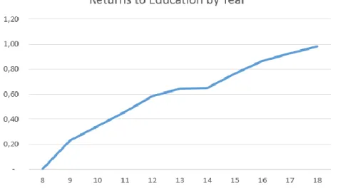
The first one is that the SOEP sample is rather limited concerning which track the participant took (a sample size of only 67317). Secondly, since the number of years it takes to obtain a diploma is different depending on the track, the analysis is not as simple as using the number of years spent studying and hence, one needs to know which track a student enrolled in to assign them a diploma after a certain number of years studying. Despite this, we can still plot the logged hourly wages against the years of schooling in 2017, seeing the following trend:
Figure 1: The logged hourly wage plotted against the year of schooling. Own calculations based on SOEP sample for 2017.
The values fit well the regression line without strong outliers. Most importantly: one can confirm that there is a positive relationship between years of schooling and one’s hourly wage. Eleven and fourteen years of studying show the highest returns relative to the fitted values line. Further, we can see that dropping out results in considerably lower returns than completing a year, as seen from those with 8.5 years of schooling (that is, those who dropped out from the 9th year) have lower hourly wages than those who completed the 9th year of school. This pattern continues with eleven, twelve and fourteen years in school. One should, however, have in mind that in Germany grade retention is legal. This means that if one’s school performance is evaluated to be less than a defined minimum, a student would have to re-take the school year. This may cause inaccuracies in the measure whereby two students may have spent the same number of years in schooling, but have a different academic attainment.
Whilst a linear relationship between log earnings and schooling is popular among scholars, Lemieux (2003) argues that since the 80s, this relationship has become more quadratic and refers to a few studies that found more appropriate the usage of a quadratic specification. Specifically, Mincer (1997) and Dechênes (2001) include a quadratic specification together with the linear one and find it improves the overall fit of the model. A reason why this relationship has become more convex is because skilled labour has higher demand thus the more educated are even better paid than before (Mincer J. A, 1997). This is supported by Acemoglu (2002) who finds that from the 40’s onwards, labour has become more skilled-biased. Further, he sees that from the last three decades, returns to schooling have been greater from the more educated due to this increased need for qualified labour.
As mentioned earlier, a completely different approach is to analyse the effects of an extension of mandatory schooling. That is, to compare the earnings of students before and after the new age when dropping out is allowed. Using this tool, Acemoglu & Angrist (2000) obtain returns as high as 10% for 1990 in the US. Similarly, Oreopoulos (2003) employ this method on a Canadian, the American and British sample. He finds that compulsory schooling laws could increase earnings by 10-14% depending on the country or region. As well as Pischke & von Wachter (2005) and Kamhöfer & Schmitz (2016) who find 0% returns to education.
The non-existent returns are rather striking, especially when they are the only country where that is found. Thus, Pischke & von Wachter (2005) investigate the existence of such a low result. Firstly. they suggest that whilst wages for 9th graders (those who studied pre- or post-reform) and 8th graders (a group consisting only of pre-reform graduates) may be the same, employers should still prefer the former since they are assumed to be more productive, however, when tested, this hypothesis is rejected since they could not find employment differences between the two groups. Secondly, since 9th graders are not being rewarded by the labour market, they would be more likely to choose self-employment. This is rejected as well. Thirdly, there is the possibility that those who took an apprenticeship (which is not counted as a year in schooling) have higher wages than their peers with the same years of study. Specifically, 9th grade attainers with an apprenticeship would have higher wages than 9th graders without one. When tested this shows not to be the case either. Ultimately, Pischke & von Wachter (2005) reach the conclusion that the reason why they obtain no returns is because of the German education system. Whereby, students obtain the skills that they will use in their employment earlier than in other education systems: “German students had learned the labour market relevant skills by the time they graduated from secondary school, while in the Anglo-Saxon countries, the most marginal students are still learning these skills at age 14 or 15” (Pischke & von Wachter, 2005). Kamhöffer & Schmitz (2016) test that theory by using the word fluency test score present in the SOEP sample. This test counts the number of animals a participant can name in 90 seconds and cite Lang, Weiss, Stocker, & von Rosenbladt (2007) who confirm that, despite its simplicity, the test is comparable to more extensive psychological tests to assess intelligence. Their results show that individuals with more years of education also show higher scores for that test (with a coefficient of 4.8%), however, this disappears when adjusting for endogeneity in school length and thus they conclude that since, as they find it, schooling does not have an effect on cognitive skills in Germany, the reason why returns are zero is due to these skills not being obtained through education (Kamhöfer & Schmitz, 2016).
2.2.3. Measuring Ability
One way to measure ability is the years of potential experience. These are given by subtracting the years of schooling and the years before an individual started their academic life (six in Germany) from the individual’s biological age. Furthermore, a
quadratic specification is added together with a linear. Murphy & Welch (1990), however, criticise the usage of such functional form saying that it understates the earnings of those with less experience whilst overestimating those in the middle of their career. They, therefore, suggest the usage of a quartic function instead and show how it provides a better fit which I will test if it applies to my sample. Alternatively, one can also simply the age of the individual. (Card, (1999))
The questionnaire in the sample used in this thesis, however, includes a variable where the participants responded how long, in years, they have worked full time. As it is more accurate than their potential years, it will be the measure of ability used.
Using uniquely the above variables: log of hourly wage, years of schooling and years of job market experience we obtain the following output:
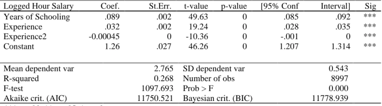
Table 2: Standard Mincer Equation Ran with OLS
Logged Hour Salary Coef. St.Err. t-value p-value [95% Conf Interval] Sig
Years of Schooling .089 .002 49.63 0 .085 .092 ***
Experience .032 .002 19.24 0 .028 .035 ***
Experience2 -0.00045 0 -10.36 0 -.001 0 ***
Constant 1.26 .027 46.26 0 1.207 1.314 ***
Mean dependent var 2.765 SD dependent var 0.543
R-squared 0.268 Number of obs 8997
F-test 1097.693 Prob > F 0.000
Akaike crit. (AIC) 11750.521 Bayesian crit. (BIC) 11778.939
*** p<.01, ** p<.05, * p<.1
Source: Own calculations based on SOEP 2017
From the table above we can see that the coefficients for the returns to education from Germans irrespective of gender and age for the 2017 sample was of 0.089. This corresponds to a return to schooling of 8.9% meaning that every year of studying, one can expect their future earnings to increase by around 9%. Concerning years of experience, since the coefficient for the quadratic specification is rounds up to zero, one year of potential experience in the labour market leads to a 3.2% increase in earnings. Overall, this model is able to explain around 26% of the variation in wages.
Comparing it to other research, Lauer & Steiner (2000) also using a sample from SOEP ran the above model in OLS and find returns of 8.3% for men and 10.8% for women. In both Lauer & Steiner (2000) and in table 2 the analysis is limited to individuals whose age was between 30 and 60 with the purpose of eliminating “the overrepresentation of the
lower educated in the sample due to earlier career starting age” (Lauer & Steiner, 2000). Another difference can be my inclusion of Eastern Germany, which their model excludes as well as their usage of potential experience18. Their higher R-squared measure also shows that their model is able to explain wage fluctuations better than the one in the above table.
Using the same model and sample Ammermüller & Weber (2005) distinguish between West and East Germany however they do not find a big difference between the coefficients (which are around 7.5%). The exception is for women who, in East Germany, have lower returns than in the West with 6.5%. Their R-squared is even lower with 15% of the variation explained.
2.3.4 Assorted Variables
In this section I discuss other variables that were included in studies that are not a measure of either experience or schooling. When calculating the returns to education in India, Duraisamy (2002) add a dummy variable if the person lived in a rural area and found that they are hindered by around 2% in income. A study in China includes variables relevant for the country in question (Li, 2003). Namely, ethnic minorities, membership in the Communist party and if the individual part-took in a re-education program (Li, 2003). They conclude that being an ethnic minority decreases one’s salary, whilst being a member of the Chinese Communist Party and participating in a re-education program increases them (Li, 2003). Likewise, for Bangladesh where Asadullah (2006) employed a dummy variable to adjust for if the individual did not follow the Muslim faith (which is the religion followed by most people in Bangladesh) and a dummy for inhabiting a rural area. Both indicated lower wages. These studies indicate that some country-specific variables may be good to adapt the data. One of the relevant factors for Germany could be the East-West divide, whereby the former had to re-integrate in a market economy whilst the latter has not had a harsh change in government since the end of World War 2. Along these lines, to increase the explanatory power of the model, one could add to the analysis the sector in which the individual is employed as well as if they are employ in
the public sector as done by some researchers (see for example Alba-Ramírez & San Segundo (1995)).
2.3.5 Instrumental Variables
This section serves to justify the usage of two-stage least squares (2SLS) with instrument variables (IV) in place of ordinary least squares (OLS) in estimating returns to education. This is due to certain difficulties in estimating wages with a regression. Specifically, omitted variable bias and endogeneity (Angrist & Pischke, 2008).
Omitted variable bias consists in inconsistencies that surge when a variable is not included in a model (Angrist & Pischke, 2008). This happens because it is not known what the true expression of wages is (Stanley & Jarrel, 1998). If a model does not control for this, the coefficients estimated will not be reliable as they may be over- or underestimated.
Harmon, Oosterbeek, & Walker, (2003) suggest factors that are often omitted (usually due to difficulties in statistically assess these variables). They mention motivation and IQ as examples of variables that may affect an individual’s earnings and schooling (Harmon et al 2003). Thus, in order to circumvent the issue of omitted variable bias, what they propose is a two-stage least squares regression whereby the years of schooling are firstly predicted, and then use that prediction as the variable for an individual’s academic career Harmon et al, 2003). This is also known as IV estimation (Angrist & Pischke, 2008). Harmon et al (2003) show that when employing IV estimation the returns to schooling increase to around 9% from 6.5% in OLS in their sample. Further, if an educational reform is considered, this value further increases to around 13%19 (Harmon, Oosterbeek, & Walker, 2003). Thereby showing that OLS underestimates returns to education and this is fixed when employing IV estimates.
As mentioned, the other problem that arises with the usage of this applying OLS to the Mincer equation is endogeneity. This happens because the variables schooling, and ability are correlated. In short, schooling either improves one’s ability—the human capital theory; or signals pre-existing ability—the screening hypothesis. Endogeneity will cause the parameters to be biased and inconsistent. One of the ways to circumvent this issue is
19 Despite this and as discussed above, Pischke & von Wachter (2005) and Kamhöfer & Schmitz (2016)
also through the usage of instrumental variables. These are to be correlated with schooling, but not with ability. Examples of used instrumental variables are family members’ education, assuming there is no generational transfer of ability, such as mother’s, father’s or siblings’ (Card, 1999) (Ashenfelter & Zimmerman, 1997); month (or quarter) of birth: which, due to compulsory schooling laws, allows students born before the schooling year to drop out, whilst forcing those born after it to continue20 (Angrist & Krueger (1991); distance to the educational institution (Kane & Rouse, 1993); tuition cost (Kane & Rouse, 1993); and smoking (Harmon, Oosterbeek, & Walker, 2003) to name a few.
Expanding on the above literature, Ashenfelter & Zimmerman (1997) control for innate family ability by using brothers’ and the father’s education to see if schooling had an effect on earnings due to family background. Their results yield that one more year of schooling leads to a 4.7% increase in earnings if taking into account family factors. The study which used month of birth to estimate earnings and education sees that those born in the first half of the year have their weekly earnings decreased by, on average, 0.7% and have 0.126 fewer years of schooling (due to them being legally allowed to drop out) (Angrist & Krueger (1991)). Kane & Rouse, (1993) who use distance to the university and its tuition cost as IV, found that one more year into schooling led to an increase in earnings by 8%. Notably, however, this is not different from their OLS result. Finally, when smoking is added as an IV, the estimation of returns to schooling increase considerable to around 20% for men (Harmon et al, 2003). However, they become more modest at around 10% when one includes only smoking at 16 years of age and even lower (8%) when controlling for the family’s background (Harmon et al, 2003).
20 Think of two students born in the same year at different months (say February and November). Assume
also that the law makes school compulsory for those under 18. In February, one student will be 18 and allowed to drop out, whilst the other will be 17 and forced to continue. The student born in November will have attained one more year of schooling. Research finds that around 25% of potential drop out stay in school and attain one more schooling year this way (Angrist & Krueger, Does Compulsory School Attendance Affect Schooling and Earnings?, 1991). Thus, those born in the first half of the year tend to have lower values in year of schooling.
3. Methodology
In this paper, returns to education are calculated through an enhanced Mincer equation. I use years of schooling for the individual’s education. The variable for ability is full-time labour market experience, which is a variable present in the sample. This variable is also included with a quadratic specification (the decision to use this specification instead of a quartic one, despite the above literature, is clarified in the results section). As mentioned earlier, country specific variables can enhance the estimation of returns to education to improve the explanatory power of the Mincer equation. Thus, I enhance the Mincer model with a variable for if the individual lives in Western Germany. Other variables related to the labour market such as the industry in which they are employed and if they work in the public sector are added to increase the explanatory power of the model. Finally, the gender of the individual is integrated into the model to capture differences in payment.
Model-wise, and as recommended by previous literature, I employ a two-stage least squares model instead of OLS. The instrumental variables used are the education attainment of the mother and father. These are expressed qualitatively and are classified as intermediate school (Hauptschule), secondary general school (Realschule), technical high school (Fachorberschule) and upper secondary school (Abitur/Gynmasium), or no school degree.
Therefore, the expression used is:
𝑙𝑛𝑖(𝑤) = 𝛼0+ 𝛽1∗ 𝑠𝑖+ 𝛽2∗ 𝑥𝑖+ 𝛽3∗ 𝑥𝑖2+ 𝛿1𝑖∗ 𝑝𝑖+ 𝛿2𝑖∗ 𝑎𝑖+ 𝛿3𝑖∗ 𝑔𝑖+ 𝛿4𝑖∗ 𝑗𝑖 Eq. 2
Where, w stands for wage, s for schooling in years, x for expected years of experience, p if they work in the private sector, a is a dummy variable if the individual ‘i’ lives in West-Germany (a for alter Bundesländer meaning old federal state), g for the gender of the individual, j for the one-digit industry code for the individual’s place of employment (j for job).
4. Data
The sample used comes from the German Socio-Economic Panel (SOEP). Using the wave from 2017 allows one to conduct an analysis that is up to date whilst at the same time being reliable in terms of data availability as more recent years may lack all or some the required variables. This wave includes 30707 individuals. After disregarding the individuals who did not answer, and those whose answers did not apply, only 14222 are wage-earners. From those wage earners I exclude those with too little work experience as well as those that are too old including only those aged between 30 and 60 as done by Lauer & Steiner (2000) and (Ammermüller & Weber, 2005) with the intention of excluding individuals who might still be in their academic life and who have not yet had time to obtain full-time work experience. Regarding years of schooling, it is not specified if it accounts for the students who had to repeat a year. Thus, we assume that all the students with the same years of schooling have the same academic achievements. In Germany, around 20% of the students will repeat a year throughout their academic life which may cause some bias in the data as one fifth is not a small proportion (Rathmann, Loter, & Vockert, 2020).
Concerning the instrument variables, the 1984 wave compiles the education of the parents of the participants. Even if not calculating the returns to education for that year, one can still use that the data for 1984 since one rarely return to schooling once graduated. Originally, this variable also included categories for those whose parents obtained their education abroad as well as those who had “other degrees”. Because these variables cannot be ranked: having an “other degree” is not superior or inferior to having either of the first four; and since education in Germany is ranked differently as in other countries, those variables are also dropped leaving the sample at 8384.
The following tables show the descriptive statistics for the used variables. Table 3 for the quantitative variables, 4 the instrument variables, 5 for the dummy variables and 6 for the categorical variable that is the sector of employment.
Table 3: Descriptive Statistics I
Variable Obs Mean Std. Dev. Min Max
Yearly salary in Euros 9021 35412.54 24325.03 150 360000
Annual hours worked 9021 1905.7 675.1 17 5383
Years of schooling 9021 13.064 2.774 7 18
Full-time labour market experience (years)
8978 16.340 10.774 0 43.7
Source: Own calculations based on SOEP 2017
As mentioned, the table above (and thus the study) excludes individuals who reported zero yearly income and whose age was outside of the 30-60 range. There are a few cases where participants reported a low amount of income, which, when divided by the hours worked awards a decimal number inferior to one. When logging this, one would obtain a negative number hence those who report an hourly wage inferior to the value of 1 are also dropped from the study. With an average year of schooling of thirteen, the average German has completed high school and, unless they enrolled in the upper track, a few years of tertiary education. Concerning ability, the sample also averages at 1906 hours worked in the whole year. This is equivalent of slightly more than seven hours per day (assuming a month has twenty-two workdays). The maximum value of 5383 seems extreme given that a year has 8760 hours which indicates that that individual spent 61.4% of the year working. Finally, the exclusion of those who are less than thirty years old still resulted in 243 people having no full-time work experience.
Concerning expectations, years of schooling should have a positive coefficient: as seen from table 1, most literature finds a positive relationship between earnings and education. The literature that finds zero returns to schooling in Germany21 employs a specification that is different from this study, thus, the coefficient being positive is the most likely outcome. Likewise, labour market experience is also expected to be positive for the same reasoning. In fact, and as an example, Lauer & Steiner (2000) and find that expected labour market experience22 4.1% or 2.5% (for men and women, respectively).
21 (Pischke & von Wachter, 2005) (Kamhöfer & Schmitz, 2016) 22 Defined as age subtracted by six and the years of schooling.
Regarding the instrument variables,
Table 4: Descriptive Statistics II
Father’s education
Mother’s Education Freq. Percent Freq. Percent
0-No school degree 311 3.65 369 4.40
1-Secondary General School 4876 57.22 4848 57.82
2-Intermediate School 1798 21.10 2205 26.30
3-Technical High school 20 0.23 15 0.18
4-Upper Secondary High School 1516 17.79 947 11.30
Total 8521 100.00 8384 100.00
Source: Own calculations based on SOEP 2017
The most common outcome for the education of one’s parent is a secondary general school degree (Hauptschule), followed by the middle track of (Realschule) and with just a few numbers less, the upper track (Abitur). The fewest chose to attend a technical high school (Fachoberschule). Importantly, most of the participants’ fathers/mothers had a school degree, only 3.65/4.40% did not.
Table 5: Descriptive statistics III
From the tables above we can see that almost 30% of Germans work in the public sectors and around one fourth of the participants live in East Germany. Gender-wise men and women are roughly equally represented by the survey. Regarding the expectations, salaries should be higher for public workers as seen from appendix 3 and for West-Germans as seen from appendix 4. The public sector offering higher wages than the public
Public Worker East Germany Gender: Man
Freq. Percent Freq. Percent Freq. Percent
[1] Yes 2572 28.51 1739 19.28 4262 47.25
[2] No 6449 71.49 7282 80.72 4259 52.75
Total 9021 100.00 9021 100.00 9021 100.00
sector may be a surprise. Indeed, there is a higher concentration of private sector individuals that earn less than the public sector’s average. However, the upper tail of those employed outside of publicly owned companies is longer. This indicates some disparities in the public sector where the majority are paid less than in the civil service, and a few have a much higher income. Whilst in the public sector, the standard deviation is lower whereby the wage differences are less remarkable. The earnings gap between men and women is estimated to be in favour of men as women have a higher, albeit decreasing, propensity of being employed in fields with lower wages (Lauer, 2000).
Table 6: Descriptive Statistics IV
1 Digit Industry Code of Individual Freq. Percent
[1] Agriculture 111 1.23 [2] Energy 124 1.37 [3] Mining 17 0.19 [4] Manufacturing 1284 14.23 [5] Construction 1082 11.99 [6] Trade 1159 12.85 [7] Transport 518 5.74 [8] Bank, Insurance 363 4.02 [9] Services 4363 48.36 Total 9021 100.00
Source: Own calculations based on SOEP 2017
The table above shows the distribution of the participants into the sectors in which they work. Most of the inquired work in the services sector which is the most common for developed countries. The least popular was mining with only seventeen of the participants employed.
Table 7: Correlation Matrix
Variables (1) (2) (3) (4) (5) (6) (7) (1) Yearly Salary 1.000 (2) Hours Worked 0.536 1.000 (3) Experience 0.355 0.410 1.000 (4) Years of School 0.401 0.114 -0.154 1.000 (5) Private Sector -0.061 -0.001 0.032 -0.214 1.000 (6) West Germany 0.111 -0.075 -0.089 0.006 -0.036 1.000 (7) If Woman -0.409 -0.443 -0.447 0.013 -0.112 -0.007 1.000
The above correlation matrix indicates an unsurprising correlation between hours worked and the yearly salary. Full-time labour market experience and years of schooling are also correlated with earnings though weaker. Women show a negative correlation with earnings which can be explained by low correlation with hours worked and labour market experience. It is likely that these values are lower for women than for men due to lower labour market participation (Colm, Oosterbeek, & Walker, 2003). The remaining variables do not show a correlation worth mentioning.
As mentioned in the section about the German education system, a student’s academic track can be an important predictor of income, however, when asked in which track they studied, most participants’ answers pertain in the “does not apply category” which would leave the variable with only 673 observations. Thus, the only reliable tool for measuring education is the years spent in schooling.
Table 8: Distribution and frequency of years of schooling in Germany in 2017
Number of Years of Education
Freq. Percent Cumulative Cumulative if
drop out 7 48 0.53 0.53 0 8.5 11 0.12 0.66 0.66 9 441 4.91 5.57 0.66 10 145 1.62 7.18 0.66 10.5 1245 13.87 21.05 14.53 11 253 2.82 23.87 14.53 11.5 1957 21.80 45.67 36.40 12 1180 13.14 58.81 36.40 13 298 3.32 62.13 36.40 13.5 227 2.53 64.66 38.93 14 253 2.82 67.48 38.93 14.5 383 4.27 71.74 43.20 15 576 6.42 78.16 43.20 16 480 5.35 83.50 43.20 17 51 0.57 84.07 43.20 18 1430 15.93 100.00 43.20 Total 8978 100.00 43.20
Source: own calculations based on SOEP 2017
Note that the table above is for the then current educational level of the sample in 2017, not what a participant had attained in that year. From table 8 we can see that most Germans spent at least one decade in education. The low occurrence of those with less
than 9 years of schooling is due to the ninth year being compulsory. Thus, those that studied for less than that immigrated into Germany with academic attainment that is below the compulsory level. The biggest concentrations are master’s degree holders (18 years) with 16%, those with exactly 12 years with 13% and those who dropped out of the twelfth and eleventh year with 22 and 14% respectively. Reasons for these propensities are puzzling as the diploma years in Germany are 9, 10 or 12/13 (for each track respectively). Whilst we do see a relatively high percentage of participants with exactly twelve years in school, which can be indicative of people deciding to join the labour market when they are done with high school, this does not happen for the years 9 and 10. What table 9 may show is that Germans continue with their education even beyond their compulsory level, even if around two fifths drop out without concluding an academic year. It may be the case that they look job a job whilst they study, and when they find one, they leave education. The exact reason for the above distribution is hard to prove without dividing the participants in their respective track, thus we are bound to theorise.
5. Results and Discussion
5.1 Returns to Education
We begin with a weak instruments test to ascertain if the variables for the parents’ education are a good tool to predict a child’s years of schooling. The null hypothesis of this test is that the instruments are weak meaning that the education of the parents is not a good predictor of a child’s academic career.
Table 9: Weak Instruments Test
First-stage Regression
summary Statistics
R-sq. Adj. R-sq. Partial R-sq. F (2,8289) Prob > F
0.2452 0.2438 0.1340
640.382 0.000 Minimum eigenvalue statistic = 640.382
10% 15% 20% 25%
2SLS Size of nominal 5% Wald test 19.93 11.59 8.75 7.25
From Table 9, we reject the null hypothesis since the F-value (640.4) is much greater than 10% critical value (19.93) thus, we can conclude that using an individual’s parents’ education as an instrument variable is appropriate.
Further, I test for a few of the possible problems when performing a 2SLS regression. Firstly, endogeneity.
Table 10: Endogeneity test
H0: variables are exogenous
Durbin (score) chi2 (1) = 18.0331 (p = 0.0000) Wu Hausman F (1,8274) = 18.0375 (p = 0.0000)
Testing for endogeneity is a way to know if using IV was better than regular OLS. The null hypothesis that the variables are exogenous would indicate that IV was unnecessary. However, since the p-value was less than 5%, we reject this hypothesis and conclude that an IV regression was necessary since the variables are endogenous. Secondly, there is the possibility that the simultaneous equations are not properly identified which would put in question the validity of the results. Thus, the test to ascertain that possibility, is found in table 11.
Table 11: Overidentification test
Tests of overidentifying restrictions: H0: The model is well specified
Sargan (score) chi2(1) =0.860475 (p = 0.3536)
Basmann chi2(1) =0.858903 (p = 0.3540)
The null hypothesis of the model being well specified cannot be rejected and thus we conclude that there is no problem of overidentification in the regression.
Running the regression stated the methodology sub-section we obtain the below table:
Table 12: 2SLS regression output
Logged Hourly Wage Coef. St.Err. t-value p-value [95% Conf Interval] Sig Schooling Years .101 .005 19.97 0 .091 .111 *** Expected Experience .025 .002 15.21 0 .022 .029 *** Expected Experience^2 0 0 -7.74 0 0 0 *** Private Sector -.106 .013 -8.26 0 -.131 -.081 *** West Germany .253 .012 20.90 0 .229 .276 *** If Woman -.103 .012 -8.60 0 -.127 -.08 ***
1-Digit Industry Code:
[1] Agriculture -.15 .045 -3.33 .001 -.239 -.062 *** [2] Energy .289 .044 6.57 0 .203 .375 *** [3] Mining .183 .107 1.71 .087 -.027 .393 * [4] Manufacturing .204 .019 10.64 0 .166 .241 *** [5] Construction .222 .02 10.98 0 .183 .262 *** [7] Transport .038 .025 1.53 .125 -.011 .087 [8] Bank Insurance .294 .03 9.92 0 .236 .352 *** [9] Services .054 .018 2.95 .003 .018 .09 *** Constant 1.196 .086 13.92 0 1.028 1.364 ***
Mean dependent var 2.776 SD dependent var 0.541
R-squared 0.348 Number of obs 8290
Chi-Square 3023.937 Prob > F 0.000
Root MSE .4372
*** p<.01, ** p<.05, * p<.1
Source: Own calculations based on SOEP 2017
Table 12 uses the trade sector as the base because its wages are the lowest after agriculture. The reason why agriculture was not used for the base is to find some indicator of how much lower returns are in rural areas which is where agriculture can be prominent. The results from Table 12 indicate that each year spent in education in Germany awards an individual with 10.1% higher income. Years of experience increase one’s wage by only 2.5% per year whilst working in the private sector decrease them, on average, by 10.6%. A reason for this may be the high prevalence of low-pay jobs found in the private sector, whilst the public sector offers more jobs which pay an average salary. We can also
see that wages are 25.3% higher in West-Germany, whilst women earn on average 10,3% less than men.
Concerning in which sector one is employed, working in the secondary sector offers higher wages, as salaries are estimated to be greater if one works in the energy, mining, manufacturing and construction sectors. The services sector shows the lowest wage after agriculture. One of the reasons why this may be is because it includes many low-skill jobs which are popular in cities (namely waiter, cashier, etc) which weigh down the average service sector wage. Furthermore, since well paid jobs in the banking and insurance jobs are separated from the rest of the services sector, Table 12 shows lower wages on other service jobs.
Comparing the results in Table 12 with articles that calculated returns to education in Germany, we can more easily relate them to the aforementioned Lauer & Steiner (2000) Ammermüller & Weber (2005) and who find positive returns to education (8 and 7%, respectively) rather than to Pischke & von Wachter (2005) and Kamhöfer & Schmitz (2016) who find low or non-existent returns. The reason is likely to be the specification. Whilst the first two studies apply a simple Mincer equation estimated through OLS, the latter two use instrument variable to adjust for if the individual was subject to an educational reform (specifically, the extension of compulsory education). Using the parents’ education as IV results in estimations closer to OLS than using the educational reform approach.
Comparing Table 12 (which employed 2SLS) with table 2 (an OLS regression), we can reaffirm the findings of Harmon et al (2003): OLS significantly underestimates the returns to education and in my case, by 1.2%. This value might seem small; however, it is 1.2% per year. The average German studies for thirteen years, thus OLS underestimates everyone’s total returns by 15.6% approximately and on average. The Hausman test in table 10 indicates that this difference is statistically significant as 2SLS is shown to be superior to OLS.
As mentioned before, some studies (for instance Pischke & von Wachter, (2005) and Murphy & Welch (1990)) find that models that have experience under a quartic function are more appropriate, however, looking at appendix 2 and comparing it to Table 12, using
a quartic specification shows a slightly higher value for the root of the mean residual squares (0.4372 for quartic and .4368 for quadratic). The difference is indeed small and comparing the coefficients of the other variables the only one that shows some discrepancy is the labour market experience (1.8% for quartic and 2.5% for quadratic). Thus, either specification adapts well to the data, though arguably, the quadratic performs slightly better.
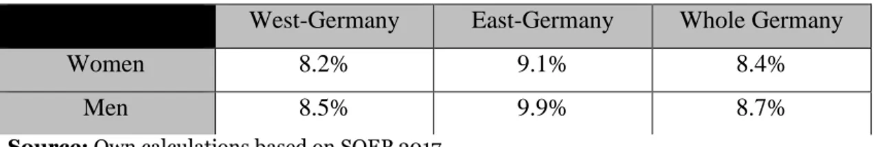
When calculating the returns to education through 2SLS for two genders and distinguishing East and West Germany, we obtain the following table:
Table 13: Returns to education in Germany.
West-Germany East-Germany Whole Germany
Women 8.2% 9.1% 8.4%
Men 8.5% 9.9% 8.7%
Source: Own calculations based on SOEP 2017
Interestingly, when differentiating between genders, the returns fall from 11.3% to under 10%, instead of averaging around the value for the whole sample. In general men have higher returns than women. This can be due to discrimination or omitted variable bias. Lauer (2000) theorised for the reasons for a wage gap between men and women in Germany for the last two decades of the twentieth century. Although her findings might be outdated, she sees that differences in human capital explain most of the payment gap (Lauer 2000). Though women still earn less than men with similar qualifications (Lauer 2000). Furthermore, Lauer points to the fact that there is evidence of some “occupational segregation” whereby women are employed in fields which offer lower pay. Despite this, the educational gap between men and women was closing when the study was performed which led to a decrease in the earnings’ gap as well (Lauer 2000). Finally, the author finds that, whilst returns to education were higher for men, returns on labour market experience were higher for women (Lauer 2000). However, these findings contradict appendix 6 and