The Value of Change : An event-study of Ownership Disclosures

I

H

T h e Va l u e o f C h a n g e

An event-study of Ownership Disclosures

Bachelor’s thesis within Finance Authors: Bergquist, Philip Lindgren, Patrik Persson, Olof Tutor: Österlund, Urban

Bachelor’s Thesis in Finance

Bachelor’s Thesis in Finance

Bachelor’s Thesis in Finance

Bachelor’s Thesis in Finance

Titl Titl Titl

Title:e:e: e: The Value of Change: An EventThe Value of Change: An Event----study of Ownership DiThe Value of Change: An EventThe Value of Change: An Eventstudy of Ownership Dissssclstudy of Ownership Distudy of Ownership Di clclcloooosuressuressures sures Author

Author Author

Author:::: Bergquist, Philip; Lindgren, Patrik; Persson, OlofBergquist, Philip; Lindgren, Patrik; Persson, OlofBergquist, Philip; Lindgren, Patrik; Persson, OlofBergquist, Philip; Lindgren, Patrik; Persson, Olof Tutor:

Tutor: Tutor:

Tutor: Österlund, UrbanÖsterlund, UrbanÖsterlund, UrbanÖsterlund, Urban Date Date Date Date: 2005200520052005----121212----1512 151515 Subject terms: Subject terms: Subject terms:

Subject terms: Stockholm Stock Exchange, efficient market hypothesis, eventStockholm Stock Exchange, efficient market hypothesis, event----Stockholm Stock Exchange, efficient market hypothesis, eventStockholm Stock Exchange, efficient market hypothesis, event study,

study, study,

study, ownershiownershiownership disclosures, passive investors, aownership disclosures, passive investors, ap disclosures, passive investors, acccctive investors, p disclosures, passive investors, a tive investors, tive investors, tive investors, private investors, institutional investors, anom

private investors, institutional investors, anomprivate investors, institutional investors, anom private investors, institutional investors, anomaaaalieslieslieslies

Abstract

Background:

Recent business paper articles observe that stocks soar when there is a change in owner-ship. The clothing company JC climbed 26% when it was announced Torsten Jansson had increased his holdings. Daydream, a computer game developer, followed this trend increasing its market value by 17% on the news that TA Capital had increased its hold-ings. In these examples, the market learned of the changes in ownership through a press release created by the acquiring entity. These pieces of news, also known as ownership disclosures, is the target of this thesis.

Purpose:

The purpose of this thesis is to investigate whether ownership disclosures result in ab-normal stock price changes. Furthermore, the aim is to find out if there are any differ-ences in returns depending on who announced the ownership disclosure. In order to fulfil this purpose, a quantitative approach was used.

Method:

A random sample of 160 ownership disclosures is gathered. 77 of these are classified as passive- and 83 as active investors. For each of these pieces of news, 183 days of his-torical stock price data is retrieved. This data is then parsed through the market model event-study framework.

Findings:

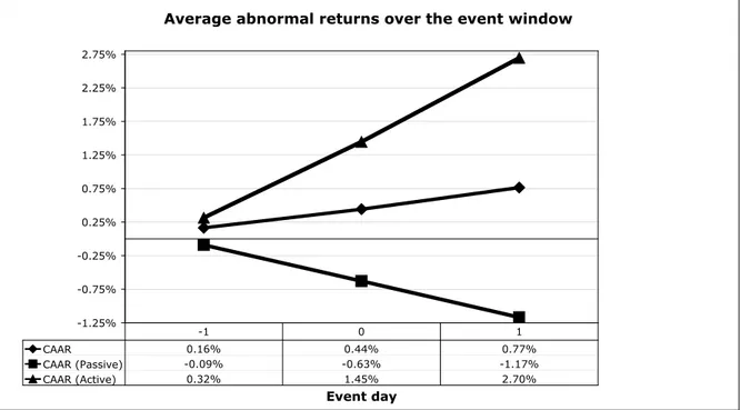
Graphically analyzing the whole sample indicates that the market is not efficient in its strong form. The same is true when dividing the sample into passive- and active inves-tors. Statistically, an abnormal return is confirmed for the active investors, but not for the whole sample or the passive investors.

Conclusion:

By looking at the price change effects of ownership disclosures, the Stockholm Stock Exchange O-list is determined to be efficient at the semi-strong level. The anomaly caused by active investors leads to the possibility of making a profit of 2.70% between day -1 and day +1 relative to the day of the ownership disclosure being sent out. It should be noted, though, that transaction costs and taxes are not taken into considera-tion.

Kandidatuppsats inom finansiering

Kandidatuppsats inom finansiering

Kandidatuppsats inom finansiering

Kandidatuppsats inom finansiering

Titel: Titel: Titel:

Titel: Värdet av förändring: En fallstudie av flaggningsmeddelaVärdet av förändring: En fallstudie av flaggningsmeddelanVärdet av förändring: En fallstudie av flaggningsmeddelaVärdet av förändring: En fallstudie av flaggningsmeddelannndendendenden Författare:

Författare: Författare:

Författare: Bergquist, Philip; Lindgren, Patrik; Persson, OlofBergquist, Philip; Lindgren, Patrik; Persson, OlofBergquist, Philip; Lindgren, Patrik; Persson, OlofBergquist, Philip; Lindgren, Patrik; Persson, Olof Handledare:

Handledare: Handledare:

Handledare: Österlund, UrbanÖsterlund, UrbanÖsterlund, UrbanÖsterlund, Urban Datum Datum Datum Datum: 2005200520052005----121212----1512 151515 Ämnesområden: Ämnesområden: Ämnesområden:

Ämnesområden: StockholmsbörseStockholmsbörseStockholmsbörseStockholmsbörsen, effektiva marknadshypotesen, hän, effektiva marknadshypotesen, hän, effektiva marknadshypotesen, hän, effektiva marknadshypotesen, hännnndelsestdelsestdelsestdelsestuuuudie, die, die, die, event

eventevent

event----study, flaggningsmeddelande, flagstudy, flaggningsmeddelande, flagstudy, flaggningsmeddelande, flagggggning, passiva investerstudy, flaggningsmeddelande, flag ning, passiva investerning, passiva investera-ning, passiva investera-a- a-re, aktiva investeraa-re, privata i

re, aktiva investerare, privata ire, aktiva investerare, privata i

re, aktiva investerare, privata innnnvesterare, institutionella investervesterare, institutionella investervesterare, institutionella investervesterare, institutionella investera-a-a- a-re, anomalier

re, anomalierre, anomalier re, anomalier

Sammanfattning

Bakgrund:

I nyligen publicerade affärstidningsartiklar nämns att förändringar i ägarskap resulterar i kraftiga kursförändringar. Kursen för klädesföretaget JC ökade 26% när det blev känt att Torsten Jansson hade ökat sitt innehav i företaget. Aktien för Daydream, en utvecklare av datorspel, följde denna trend när dess marknadsvärde ökade 17% vid tillkännagivan-det av att TA Capital gjort en förändring i sitt ägarskap. I dessa exempel tog marknaden del av ägarförändringarna genom ett pressmeddelande utskickat av den köpande parten. Ett annat ord för dessa utskick är flaggningsmeddelanden.

Syfte:

Syftet med denna uppsats är att undersöka huruvida flaggningsmeddelanden resulterar i abnormala aktiekursförändringar. Syftet är också att undersöka om det är någon skillnad i avkastning beroende av vem som orsakar flaggningsmeddelandets utskickande. För att uppfylla syftet användes en kvantitativ metod.

Metodval:

Ett slumpmässigt urval om 160 flaggningsmeddelanden drogs fram, varav 77 klassades som passiva- och 83 som aktiva investerare. För envar av dessa samlades 183 dagars hi-storisk kursdata in som sedan behandlades med hjälp av en marknadsbaserad händelse-studie (event-study).

Resultat:

Genom att grafiskt analysera hela urvalet noteras att marknaden inte är effektiv i sin starka form. Samma resultat nås då urvalet delas upp i passiva- och aktiva investerare. Statistiskt bekräftas dock endast den aktiva delmängden.

Slutsats:

Genom att undersöka prisförändringseffekterna av flaggningsmeddelanden konstateras att Stockholmsbörsens O-lista är mellanstarkt effektiv. Anomalin som orsakas av aktiva investerare ger upphov till möjligheten att tjäna 2.70% mellan dag -1 och +1 relativt den dag då flaggningsmeddelandet skickades ut. Det bör dock noteras att hänsyn inte tagits till transaktionskostnader och skatter.

Table of contents

1

Introduction... 6

1.6.2 The event-study research approach ... 9

2

Theoretical Framework ... 11

2.1 The efficient market hypothesis... 11

2.1.1 Three forms of market efficiency... 11

2.2 Anomalies ... 12

2.2.1 Arbitrage ... 13

2.2.2 Value vs. Growth ... 14

2.2.3 Seasonal anomalies – the January effect ... 14

2.3 Testing anomalies ... 15

2.4 Disclosure of market information ... 15

2.5 Previous event-studies ... 16

2.6 Investor classes ... 17

3

Methodology ... 18

3.1 Data collection... 18

3.1.1 Ownership disclosure data ... 18

3.1.2 Historical stock price data... 18

3.2 An introduction to basic statistical terminology ... 19

3.3 Underlying assumptions of the event-study model ... 20

3.3.1 Identification of the events of interest and definition of the event window... 20

3.3.2 Selection of sample set of firms to include in the analysis ... 21

3.3.3 Prediction of a “normal” return during the event window in the absence of the event ... 23

3.3.4 Estimation of the abnormal return within the event window ... 24

3.3.5 Statistically testing the abnormal return ... 26

3.4 Result analysis ... 27

3.5 Research credibility ... 28

4

Empirical Findings and Analysis ... 30

4.1 Obtaining the data ... 30

4.2 Practical complications in gathering data ... 33

4.3 Running the calculations ... 33

4.4 Graphical and statistical analysis ... 35

4.4.1 Passive Investors... 36

4.4.2 Active Investors ... 36

4.5 Analysis summary ... 38

5

Final conclusions ... 40

5.1 Result reflections... 41

5.2 Methodological reflections suggesting further studies ... 42

References... 46

Appendix I: Example of Ownership Disclosure ... 50

Appendix II: Sample gathered from Affärsdata ... 51

Appendix III: Companies with new names... 73

Appendix IV: Numerical presentation of empirical

findings ... 74

Figures

Figure 1-1 – MacKinlay's five steps of an event-study (Dasgupta et al., 1997)10 Figure 2-1 – Deviations from the 60-40 cash-flow parity (Froot & Dabora,

1998 as cited in Shleifer, 2005) ... 13

Figure 2-2 – Performance of value- versus growth stocks in different companies (Fama & French, 1998) ... 14

Figure 3-1 – The event-study model time line (MacKinlay, 1997) ... 20

Figure 3-2 – Event sampling technique summarized ... 22

Figure 3-3 – Analytical interpretation model of the event-study result... 28

Figure 4-1 – A graphical view of the result ... 35

Figure 4-2 – The analytical path to the final conclusion ... 39

Tables

Table 4-1 – First sampling round – sampling distribution ... 30

Table 4-2 – First sampling round - removal of overlapping events... 31

Table 4-3 – Second sampling round – sampling distribution ... 31

Table 4-4 – Second sampling round - removal of overlapping events... 31

Table 4-5 – Third sampling round - sampling distribution... 31

Table 4-6 – Third sampling round - removal of overlapping events... 31

Table 4-7 – Total number of usable events ... 32

Table 4-8 – Final sample of usable events... 32

Table 4-9 – Abnormal returns over the event window ... 34

Table 4-10 – The final result tested for significance ... 36

Table 4-11 – Passive investors' cumulative average abnormal returns statistically tested ... 36

Table 4-12 – Active investors' cumulative average abnormal returns statistically tested ... 37

Table 5-1 – Arbitrage opportunity created in the sample of active investors 41

Equations

Equation 2 – Mean risk-adjusted market premium ... 24

Equation 3 – The average security return over the estimation window ... 25

Equation 4 –The average estimation window market portfolio return... 25

Equation 5 – Estimating the systematic risk ... 25

Equation 6 – Error variance for the estimation period ... 25

Equation 7 – Variance of the estimated abnormal return for large samples . 25 Equation 8 – Average estimated abnormal return for period t ... 26

Equation 9 – Variance of the period-t average abnormal return... 26

Equation 10 – Cumulative estimated average abnormal return... 26

Equation 11 – Total variance for the cumulative average estimated abnormal return ... 26

Introduction

1

Introduction

“The Opcon share climbed seven percent on the announcement that the IT-legend Mats Gabrielsson in-creased his holdings in the company, thereby controlling 26% of the votes”1

1.1

Background

A capital market allows the redistribution of resources from areas of surplus to areas of scarcity, such as developing industries. Two categories of means have emerged to fulfil this objective: the primary- and the secondary market. Money earned in the secondary market, most simply exemplified as stock exchanges, is used to support the primary market. The primary market is used when companies are first listed on a stock exchange (Bodie, Kane, Marcus & Perrakis, 2003).

For the objective of providing capital to the developing sectors, the primary market would be sufficient. However, investors require the possibility to trade and diversify their hold-ings. This is where the secondary market becomes important. When trading in this secon-dary market, an essential concern for investors is how to price these securities (Urwitz & Viotti, 1988).

According to the efficient market hypothesis, the price of a stock reflects all information available about the underlying company (Bodie et al., 2003). Fundamental analysts, on the other hand, claim that the current and future cash flow of a company is what really matters (Cottle, Murray & Block, 1988). Intuitively, a combination of these two makes sense – cur-rent and future cash flows are impacted by information on what happens to the company, as well as the industry in which it operates.

In a chronicle published in the Swedish business paper Dagens Industri, the author Tomas Linalla reflects on the success of the businessman Laurent Leksell who did a turn-around in the Swedish medical company Elekta. When the market learned Leksell was to buy a stake in the public offering of another public company, Karo Bio, its stock price climbed on the news (Linnala, 2005). Furthermore, the publicly listed investment firm Novestra, recently aquired 5.2% of the shares in Scribona. Scribona climbed 4% on the news (Nyhetsbyrån Direkt, 2005). More examples of price movements due to changes in ownership are de-scribed in Table 1-1 below (Thulin, 2004; Hedensjö, 2003; Hammarström, 2002; Huld-scheiner, 2002; Linnala, 2005; Granström, 2004).

Acquirer Target firm News impact on stock price

Torsten Jansson JC +26%

Symphony Intentia +8%

TA Capital Daydream +17%

Traction Thalamus +12%

Proventus Brio +1%

Laurent Leksell Ortivus +15%

Table 1-1 – Price changes resulting from changes in ownership

From this news summary, it appears that the market connects a change in ownership with boosts in future cash-flows.

1.2

Problem discussion

It appears that new information instantaneously is evaluated, valued and incorporated into the price of a stock. The piece of news this thesis will focus on is the disclosure of acquisitions and transfers of shares2_{, henceforth denoted as ownership disclosures.}

The price movements mentioned in the preceeding examples could be purely random (Ac-zel, 2002). It could also be that they are somehow related to the disclosure of change in ownership. For any useful interpretation of the observed return, be it positive or negative, to be made it must be contrasted against the market return for the same period. Any return exceeding the market return3 is considered abnormal (MacKinlay, 1997). This discussion is formalized through the following question:

1. Does the announcement of an ownership disclosure abnormally affect the price of the underlying se-curity?

Finally, it is implied above that Laurent Leksell has taken an active role in managing his previous holdings to thereby strengthen the financial performance of these companies. He is, as Brigham and Daves (2004) puts it, an active investor.

On the other side, there are passive investors, who try to predict the future prospects of a firm and make an investment if the outlooks are good. These investors do not take an ac-tive managerial role, but instead vote with their feet – sell of their holdings – if the man-agement performs poorly (Brigham & Daves, 2004). A question is therefore raised:

2. In the case of abnormal returns being observed, will these differ depending on the investor being classified as either passive or active?

1.3

Purpose

The purpose of this thesis is to investigate whether ownership disclosures result in abnor-mal stock price changes. Furthermore, the aim is to find out if there are any differences in returns depending on who announced the ownership disclosure.

1.4

Perspective

Profiting from beforehand knowledge of changes in ownership could be seen from four perspectives.

Firstly, an insider4 _{already holding a stake in a company might buy more shares hoping for}

the stock price to soar on the news of his or her increased ownership. This person is not very likely to be able to profit from the short-term returns, as the profits made could be offset if the market perceives him or her selling as a sign of the firm not going well (Bodie et al., 2003).

2 _{This is an official translation of the Swedish concept ”flaggningsmeddelande” (FöretagsJuridik Nord & Co}

AB, 2004).

3 _{Another word for the market return is ”normal” return or expected return (MacKinlay, 1997; Bodie et al.,}

2003).

4 _{An insider is defined as someone who possesses firm-specific knowledge such as financial status or future}

Introduction

Secondly, someone acquainted with an insider having overheard news of him/her increas-ing, or decreasincreas-ing, the ownership in a company might trade on the information. According to the Insider Trading Act (2005), trading on news that could affect a stock price is illegal if the information has not previously been communicated to the market. In other words in a market where the regulation works, this perspective will not exist.

Thirdly, an investor might have observed a previously successful businessman, or busi-nesswoman, holding a stake in a firm. The same investor might buy some shares on the suspicion that this businessperson might increase his or her holdings in the firm, leading to an abnormal return on the news.

Finally, an investor might observe a previously successful businessman, or businesswoman, disclosing a change in his or her stake in a company. The same investor then has the possi-bility to imitate this person by buying or selling shares in accordance with the observed change in ownership. This, supposedly, would lead to an abnormal return.

This thesis should be seen as a tool for investors belonging to the third and fourth perspec-tive as they are the only ones who legally can make a profit from ownership disclosures.

1.5

Delimitation

In order to explore the effects of ownership disclosures in stock prices, this thesis delimit its scope to Sweden and the Stockholm Stock Exchange. The reason for this is multifac-eted.

Firstly, the preference for the Swedish Stock Exchange is based on the fact that the authors of this thesis, through daily news in business papers and on the Internet, are surrounded by information regarding changes on the Stockholm Stock Exchange and the companies listed there. Therefore, a feel and knowledge about the market is present. This, assumably, leads to a deeper insight and understanding in the analysis than would have been the case if the US-, or UK-market had been targeted.

The explanation for choosing specifically the OMX listan (henceforth denoted as the O-list) is two-fold. Firstly, the O-list is exempted from wealth capital taxation (Skatteverket, 2004), which can be thought of as a reason for private investors to focus their interests on this list, instead of lists where the 1.5 percent wealth tax (Skatteverket, 2005) is levied. It should be noted that some companies during the 90’s were listed on the now abandoned OTC-list, and others are now found in the Attract40-list. These two lists are, or were, a part of the O-list and are therefore included (P. Keusch, Personal Communication, 2005-28-11; OMX, 2005c; OMX, 2005d).

A second reason for choosing the O-list is a combined effect of market capitalization and market regulations. More specifically, A-list companies have a minimum market value re-quirement of SEK 300 million to be enlisted. No such lower market capitalization limit ex-ists for O-list companies (Föreningssparbanken, 2005).

Also, if an investor buys into five percent or more of a company, an ownership disclosure has to be sent out. The same is true if an investor sells its shares and thereby ends up with total holdings of less than the five percent threshold (FöretagsJuridik Nord & Co AB, 2004). The authors therefore reason that there will be more ownership disclosures, a larger sample, sent out from the O-list as it is less costly for a smaller investor to buy a stake of five percent or more on this list than it would be investing in A-list companies. This large

sample is important to reduce the sampling error, or, in other words, to increase the trust-worthyness of the statistical results (Aczel, 2002).

The current legislation regarding ownership disclosures was put into effect in 1991 (Finan-cial Instruments Trading Act, 1991). The rules regulating ownership disclosures, however, were first published in 1994 (FöretagsJuridik Nord & Co AB, 2004). Incidentally, the news database used in this study, Affärsdata, only contains ownership disclosures from 1994 and onward. Therefore, the time period looked at is 1994-01-01 to the sampling date, 2005-11-19.

Finally, taxes and transaction costs are not taken into consideration in the results of this thesis.

1.6

Methodological positioning

The stated purpose calls for a model to test for a statistically significant relationship be-tween ownership disclosures and stock price returns. This is in line with the understanding of a quantitative analysis as defined by Saunders, Lewis and Thornhill (2003). Davidsson (2004) takes their definition, that data is collected in a standardized and numerical form for further statistical analysis, one step further by claiming that quantitative methods are appli-cable in cases of large observation sets, allowing for general conclusions to be drawn. In contrast to what is mentioned above is the area of qualitative research. In their most ex-treme form, these types of studies try to create an explanation for a problem by building general concepts out of non-standardized data. The notion of non-standardized data, as gathered from conducting interviews or doing a case study, is very important here. It allows for a more vivid explanation of reality than does summarizing it using numbers (Saunders et al., 2003). Put differently, qualitative methods builds theories and quantitative methods confirm them (Bryman, 1995/1997).

To sum up the discussion above, a statistical model will be used to test the validity of the theoretical framework. Thus, the study is classified as quantitative.

1.6.1 Literature study

To find methods that would explain the relationship between information and market reac-tions, previous theses in finance in general and the efficient market hypothesis in particular were studied. Also browsed were books in corporate- and investment finance. By doing so, it became evident that the event-study methodology is a widely used technique to do nu-merical analysis of newly published information.

To find other event studies, the keyword ”event study” was run through the following da-tabases: ABI/Inform Global, Digitala Vetenskapliga Arkivet (DIVA), Ebrary, Google, Google Scholar, JSTOR, JULIA and the Social Sciences Citation Index.

1.6.2 The event-study research approach

In the results of the queries mentioned above, two articles were often quoted: “Event Stud-ies in Economics and Finance” (MacKinlay, 1997) and “Problems and solutions in con-ducting event studies” (Henderson, 1997).

Introduction

According to MacKinlay (1997), the main underlying assumption of the event-study model is that if news communicated to the market contains any useful and unexpected content, an abnormal return will occur. Henderson (1990, p. 301) supports MacKinlay and gives a good reason for using event studies:

“The event-study is a classical design. Classic designs are simple and elegant, and, above all else, functional. The event-study has become a classic because it works. It can be used under less than perfect conditions and still produce reliable results.”

MacKinlay (1997) has categorized the event-study methodology into five different steps, summarized in a study conducted by Dasgupta, Laplante and Mamingi (1997). These steps, reprinted in Figure 1-1, will be followed in this thesis.

1: Identification of the events of interest and definition of the event window

2: Selection of the sample set of firms to include in the analysis

3: Prediction of a normal return during the event window in the absence of the event

4: Estimation of the abnormal return within the event window, where the abnormal return is defined as the difference between the actual

and predicted returns

5: Testing whether the abnormal return is statistically significant

2

Theoretical Framework

This chapter starts out in the efficient market hypothesis. From there, the discussion progresses through a number of deviations from the hypothesis and explains how to test for these anomalies. Moreover, an over-view of how the event-study model has been used in previous research is presented. Finally, a theoretical dis-cussion on passive- and active investors is held.

2.1

The efficient market hypothesis

The efficient market hypothesis states that all available information is reflected in the total value of the capital market, implying any investment made will have a zero net present value. Put differently, there is no information asymmetry – all trading parties will have the exact same information and securities are fairly priced (Ross, Westerfield, Jordan and Rob-erts, 2005b). Wärneryd (2001) adds that new information will be acted upon instantane-ously by the market.

This market action to new information can be explained by dividing information into two classes: expected and unexpected. If a stock price change occurs, the information is unex-pected. Expected information, however, is already discounted into the price and will have no effect (Ross et al., 2005).

Shostak (1997) questions these assumptions when introducing that even though a news item is expected it can still affect share prices. The author gives the example of an expected interest rate change administered by the Central Bank of an arbitrary country. This, sup-posedly, leads to an upward turn of the economy.

In a separate discussion, Shostak (1997) argues that occasionally information will first be understood by a few individuals (insiders), and then spread to the rest of the market. Hence, in these cases of private information, prices will not be adjusted even if the infor-mation released is considered to be unexpected by the market.

2.1.1 Three forms of market efficiency

Observations have shown that information is not always incorporated instantaneously (Ross et al., 2005b) These observations create a new question, to what extent is the market efficient? According to Ross et al. (2005a), there are three different classes of market effi-ciency: weak-, semi-strong-, and strong form, where each class incorporates different kinds of information into the prices of securities.

2.1.1.1 Weak market efficiency

An understandable definition of the weak form of market efficiency is presented by Fama (1991, p. 5): “[…]returns are unpredictable from past returns or other variables”. Mathe-matically,

Pt_{= P}t − 1+ E(R)t − 1+εt

Pt is the current price

Pt − 1 is the price in the previous measurement period

Theoretical Framework

εt is an explanation variable of any randomness occurring during the interval

The time interval used is of less importance and can be everything from split seconds up to several years (Ross et al., 2005a)

In conclusion, in a weak-form market, it is futile to look at historical data to find mispriced securities. In other words, technical analysts have no chance of earning excess returns in this market form since all available data is already incorporated into the price of a stock (Shostak, 1997).

2.1.1.2 Semi-strong market efficiency

In this form of market efficiency, prices of stocks reflect all publicly available information, such as the information found in annual reports, press releases and analysts’ reports. His-torical stock price data is also included. Also, if the semi-strong form of efficiency is valid, the criterion for weak form is also fulfilled (Ross et al., 2005a).

This form of market efficiency has been debated, among others by Ross et al. (2005b), since it implies that if a market of semi-strong form exists, then fundamental analysts such as mutual funds managers can not earn excess returns by interpreting publicly available in-formation. The reason for this is that the information is already reflected in the price of a certain stock.

Ross et al. (2005a) describes two ways of testing for semi-strong efficiency: Either make an event-study or make a comparison between the market index and a mutual funds index. The latter technique is testing whether mutual funds managers are able to outperform the market index. Tests have shown that in accordance with the efficient market hypothesis, mutual fund managers are not able to beat market indexes (Ross et al., 2005b).

2.1.1.3 Strong market efficiency

Information that in the weak- and semi-strong markets was known exclusively to insiders is now regarded as information known to all. Put differently, there is no non-public informa-tion regarding a company (Ross et al., 2005a).

Research has shown that there are deviations from the criteria of strong market efficiency. Niederhoffer and Osborne (1996), for example, show that New York Stock Exchange spe-cialists use inside information to make advantageous trades. Scholes (1972) conclude that corporate insiders have access to information that is not reflected in the price of securities. These studies can be seen as an indication of that a strong market is hard to achieve (Sarno, 2004).

Supporting this claim are Grossman and Stiglitz (1980), who argue that for the strong form to apply, the cost of getting prices to reflect all available information in the market must be zero. Jensen (1978) argue that if the cost of receiving insider information is higher than the profits made from it, strong markets are less likely to be observed.

2.2

Anomalies

Ever since the efficient market hypothesis was presented, it has been used by researchers to explain how markets incorporate different kinds of information into the price of securities. There are also cases where fluctuations in the market cannot be explained with the efficient

market hypothesis, which has lead to a large body of questioners of the theory. These non-explainable deviations from the theory is referred to as anomalies (Cataldo, 2000).

Ross et al. (2005a) argue that the three different forms of market efficiency do not apply in reality. Below is presented an empirical discussion of different anomalies.

2.2.1 Arbitrage

Assets of equal fundamental value shall be equally priced even if they are traded in different markets. Occationally there are price discrepancies between markets.

If an investor finds two assets with the same fundamental value but at different prices, a strategy of buying low and selling high at the exact same point in time will lead to a risk-free profit. This type of investors is also called arbitrageurs (Sharpe & Alexander, 1990). An example of this phenomenon is the American Depositary Receipts, which has been noted to be traded at different prices in different market places. In the United States, a re-ciept has one price but when it is traded on a foreign market, it has a different price, al-though being adjusted for differences in exchange rates (Shleifer 2005).

A more extensive example is the joint-venture between Royal Dutch Petroleum and Shell. The companies agreed that the cash-flows of the new company would be kicked back to the holding companies at a 60-40 ratio. As the two original entities continued to be publicly traded, it was expected that the stock of Royal Dutch Petroleum’s equity would trade at a 1.5 ratio compared to that of Shell Transport (Shleifer, 2005).

Figure 2-1 – Deviations from the 60-40 cash-flow parity (Froot & Dabora, 1998 as cited in Shleifer, 2005)

In figure 2-1, the deviations of the Royal Dutch Petroleum stock from its fundamental value (based on the 60-40 cash-flow split) is displayed. It is noted that Royal Dutch Petro-leum was relatively underpriced in the period from 1980 up until 1984 where it became overpriced.

These are straightforward examples of the efficient market hypothesis not always applying – else it would be completely clear to the investors what the stock prices should be relative the other company and deviations would instantly be adjusted.

Theoretical Framework

2.2.2 Value vs. Growth

Many papers over the years have come to the conclusion that it is possible to gain excess returns by investing in value stocks rather than growth stocks. Value stocks are defined as stocks with a low P/E-ratio (price per share-to-earnings per share) and/or stocks with low P/B-ratios (price per share-to-book value per share). Conversely, growth stocks are those with high P/E- and P/B-ratios (Ross, 2005).

Ross (2005b) argues that earning excess returns this way should not be possible according to the efficient market hypothesis. That is, using a specific investment strategy should not be able to beat the market index.

The opposite has however been shown possible in studies by Fama and French (1998). In their study they argue that in twelve out of thirteen major markets worldwide, during the 1975-1995 period, value stocks outperform growth stocks.

0 5 10 15 20

United States Japan United Kingdom France Germany

Growth Value

Figure 2-2 – Performance of value- versus growth stocks in different companies (Fama & French, 1998)

It is evident from the graph that the value stocks outperform the growth stocks. This result contradicts the efficient market hypothesis and has been criticized by Kothari and Sloan (1995), who argue that this discrepancy in the value of stocks is merely an effect of bias in information databases and not due to true market inefficiency.

2.2.3 Seasonal anomalies – the January effect

A completely different set of deviations from the market hypothesis are seasonal anoma-lies. Cataldo (2000) states that over the past 50 years, predictable seasonal patterns have been detected and confirmed statistically. These patterns include, but are not limited to, the January-, The Day-of-the-week-, the Holiday- and the Turn-of-the-month effect. One of these will be further exemplified.

Malkiel (2003) notes that during the first month of the year, stock market returns are un-usually high – the January effect. It can most simply be explained by the fact, that at the end of the previous year, investors sell the stocks in their portfolio that have performed poorly to reduce the total taxable capital gain.

This behavior push the prices down and when investors buy the shares back at the begin-ning of the year, the prices rebound and create an abnormal return for those buying the stock at the beginning of the following year.

Other explanations for the January effect are discussed by Cataldo (2000). Two of the ex-planations discussed by the author are seasonal information and window dressing. Seasonal

information is explained as the difference in information flow during the year and window dressing is explained to be the manipulation of income by institutional managers in order to maximize earnings.

Opponents to the efficient market hypothesis argue that seasonal effects such as the Janu-ary effect are proof of market inefficiency. If the market was efficient, it should clear this inconsistency with investors selling their shares short right before the rest of the market starts selling out, and later on, also buy back the shares just before everybody else does. (Malkiel 2003).

2.3

Testing anomalies

One way of testing the anomalies mentioned above is by conducting a random walk test. It is based on the assumption that the variance increases lineary with the number of observa-tions. For instance, the variance of Xt – Xt-2 is double that of the period Xt – Xt-1. That is,

the former time period is double the length of the latter and therefore the variance is twice as large. Thus, by taking half of the variance of Xt – Xt-2, and statistically comparing the

value to the variance of Xt – Xt-1 the validity of the theory can be tested (Lo & MacKinlay,

1988).

Calendar anomalies, such as the January effect, can be tested using multi-variate regression models including dummy variables (Pearce, 1996). To test the superiority of growth-/value-strategies, two mutually exclusive portfolios are set up – one containing stocks having a price/earnings-growth of over one and one portfolio where the ratio is less than one. It is then assumed that one of these strategies will outperform the other and that an investor uses this knowledge to, at the same time, sell (short) the overvalued portfolio and buy (long) the undervalued portfolio (Chahine & Choudhry, 2004).

Finally, as already implied, the event-study model is frequently used to test the effect of in-formation on stock prices (MacKinlay, 1997). These previous event-studies can be placed in two categories depending on the type of information they concern:

• The stock price effect of information released by a company • The stock price effect of news concerning a company

The communication of information to the market is covered by different regulations de-pending on which of the two types of information that is to be communicated. Therefore, an understanding of the different regulations needs is required before entering the area of previous research.

2.4

Disclosure of market information

The reason the first type of news, information released by a company, exists is found in the Listing Agreement for the Stockholm Stock Exchange. It states that all relevant informa-tion concerning the company and its operainforma-tions must be conveyed to the market (Stock-holm Stock Exchange Listing Agreements, 2005). More specifically, the guiding rule states that “information that is likely to materially influence the valuation of the Company’s listed securities may not, other than in special cases, be disclosed other than through publication” (Stockholm Stock Ex-change Listing Agreements, 2005, p. 3).

Theoretical Framework

This quote implies that all information affecting the company valuation should be disclosed in financial reports or through other disclosures. As defined by the Listing agreement (OMX, 2005a), information affecting the company valuation could concern financial statements, including items as earnings announcement, proposed dividends or share repur-chases. The information could also be of managerial kind, as for example the proposed composition of the board of directors (OMX, 2005a).

The release and content of the second type of news, where ownership disclosures are in-cluded, cannot be affected at all by the listed company – it is caused by a third-party such as an investor. To create a background understanding of ownership disclosures, the rules and regulations surrounding the piece of news is presented below.

There are two instances regulating the formatting and phrasing of an announcement of ownership changes to the market (FöretagsJuridik Nord & Co AB, 2004): the Financial In-struments Trading Act (1991:980) and the Rules Concerning the Disclosure of Acquisitions and Transfers of Shares, Etc (the NBK rules). They are not mutually exclusive but the lat-ter is more generous in lat-terms of conveying information to the market.

The major differences between the two are that the Financial Instruments Trading Act only requires an announcement to be made when there has been a change in the number of votes for an owner. More specifically when certain percentage ownership thresholds are passed (FöretagsJuridik Nord & Co AB, 2004). These thresholds are 10, 20, 33 1/3, 50 and 66 2/3 percent (Financial Instruments Trading Act, 1991).

Additionally, the NBK rules call for an announcement to be made when an owner has changed his/her/its percentage ownership of the share capital and when ownership thresh-olds in multiples of five have been passed (for example 15, 10, 5 etc percent). These rules are a part of the contract signed between a company and the Stockholm Stock Exchange when it is floated. Moreover, an investor trading at the exchange also have to adhere to these rules (Avanza, 2005). Finally, the rules state that the announcement of a change in ownership, at the certain thresholds as mentioned above, must be made 9 a.m. the day fol-lowing the transaction to an established news agency, a nation-wide paper and to the Stockholm Stock Exchange. (FöretagsJuridik Nord & Co AB, 2004). In other words, the market will be properly informed of a major change in ownership.

It is now clear that two different regulations cover how to communicate news events to the market. They differ with regards to which entity sends out this information. The scope of this thesis is, however, ownership disclosures as covered by the NBK-rules. Since no event-studies on ownership disclosures have been found, the purpose of the previous research presented next is to serve as an introduction to the strength and general usability of the model.

2.5

Previous event-studies

Abdel-Khalik and Ajinkya (1982) researched if financial analysts held an informational ad-vantage after revising earnings forecasts, resulting in abnormal returns. This was done in an event-study where the capital market was segmented into a primary and secondary group. The primary group was defined as the clients to the firm revising the forecast, and the sec-ondary group was everyone else. The study concluded that the strong form market effi-ciency did not hold. Put differently, abnormal returns could be generated by being a client to the revising firm. All other market participants, however, would not benefit from the earnings revision, thus confirming the semi-strong market efficiency.

Jaffe (1974) performed a statistical test on the usefulness of insider information. Two dif-ferent studies are discussed: one where the result is that this type of insider knowledge does not lead to abnormal returns and another where it does. In addition to these studies, Jaffe (1974) adds the effects of transaction costs to the discussion. His findings concluded that insiders do possess special information, enabling them to make abnormal returns. This is, again, a confirmation of the semi-strong form of market efficiency. Jaffe (1974) finally concluded that profits are reduced by 40% due to transaction costs.

Another area where event studies frequently have been used is in the evaluation of Mergers and Acquisitions (M&A). Paulter (2003), mention stock market studies as a common ap-proach of how to measure the success of mergers and acquisitions. Loughran and Vijh (1997) measured the five year stock returns following the acquisition for the aquiring firms. According to their findings, the stock returns differed significantly depending on the pay-ment method. They found negative abnormal returns of -25% following the stock mergers and positive abnormal returns of +62% following cash offerings.

Clients to analysts firms, insiders and acquiring firms are all investors. In the background discussion, a differentiation is made depending on if the investors are active or passive. To gain a deeper understanding of the problem, a more detailed discussion of investor classifi-cation is presented next.

2.6

Investor classes

The classification of different type of investors is a diverse area. Shleifer and Summers (1990) make a distinction between arbitrageurs and noise traders. Barber and Odean (2001) divide investors into two categories: professional and individual. Griffin, Harris and Topa-loglu (2003) denote investors as either being institutional or individual. In common for their different definitions is that the arbitrageurs, institutional and professional investors are assumed to trade on a rational basis after conducting a valuation procedure. Noise traders belong to the category private investors (Barber, Odean & Zhu, 2003).

Davis and Steil (2001) further defines institutional investors as specialized in managing sav-ings on behalf of small investors collectively. This means that small investors authorize an institution to invest their savings on the capital market in accordance with some predeter-mined objective. The rationale behind this is uncomplicated; by doing so, the small investor can achieve a diversified portfolio although his resources may be scarce. To achieve a di-versified portfolio for a small investor would otherwise require investments in 30 different firms (Ross et al., 2005).

Just like any investor, the institutional investors are entitled to execute their voting powers. However, they do not want to be tied up with specific investments since they want to tain the ability to sell their shares at any time. Therefore, institutional investors rarely re-quire representation in the board of directors. As a consequence, their efforts regarding the monitoring will be limited to some extent. This behavior is known as “voting with the feet”, thus selling their shares when the firm performance is poor (Brigham & Daves, 2004).

According to Feeney et al (1999), private investors, also denoted as informal investors, tend to make their investment decisions based on different criteria than the institutional fund managers. As example, they mention that private investors tend to monitor their holdings closer than their institutional peers – they are taking an active role in their holdings.

Methodology

3

Methodology

In this chapter, the method by which the data has been gathered is described and analyzed. Also, since this thesis relies heavily on the event-study model, its underlying assumptions are presented. Finally, a model ex-plaining how the parsed data will be analyzed is presented.

3.1

Data collection

Regardless if a quantitative or qualitative study is conducted, its input can be allocated to ei-ther of two classes: primary- or secondary data. Primary data is obtained through direct ob-servations: by counting the number of people entering a building or by conducting an in-terview. Data used in a different setting than it was originally intended for is defined as secondary. An example of this can be data collected from a database.

Secondary data can be further classified into being raw or compiled. Whereas raw data is completely untouched, compiled data has received some kind of processing to make inter-pretation easier (Saunders et al., 2003).

As previously mentioned, two inputs are required by the event-study model: events, in this case ownership disclosures, and historical stock price data, both gathered from databases. Using the above classifications, the data is secondary and compiled.

3.1.1 Ownership disclosure data

According to the rules regulating ownership disclosures, the Stockholm Stock Exchange as well as a major national news agency must receive the press release of the change in owner-ship (FöretagsJuridik Nord & Co., 2004). Some of these major news agencies are Ticker, Tidningarnas Telegrambyrå (TT) and Direkt. The rules, however, do not state which of these agencies the press release should be sent to. If, for instance, Ticker would have been chosen as the source of ownership disclosure data, companies sending to any of the others would have been excluded from the study. Then it would not be possible to state that the whole O-list has been the targeted population of this study.

Due to the problem mentioned above, a database covering all the major news agencies’ press releases was needed. Affärsdata is such a database, receiving and publishing, amongst other things, ownership disclosures sent out by major Swedish news agencies such as Ticker, Tidningarnas Telegrambyrå (TT) and Direkt. A typical ownership disclosure press release, as presented in Affärsdata, can be found in Appendix 1.

3.1.2 Historical stock price data

When an ownership disclosure has been isolated and an event window defined, the “nor-mal” (expected) return for that window needs to be estimated. This is done by using his-torical stock price data (closing prices) for the company in question. All the target compa-nies of the study are listed on the Stockholm Stock Exchange. Hence, the needed data will be downloaded from their webpage.

It could be argued that Affärsdata or Yahoo Finance could be used to obtain the historical stock price data. However, they both use secondary and complied data from the Stockholm Stock Exchange. Since it cannot be determined how the data is transferred to these data-bases and processed before being displayed on the Affärsdata or Yahoo web sites, the

au-thors question the quality of the data. Hence, Stockholm Stock Exchange is most likely the best source to use.

3.2

An introduction to basic statistical terminology

Before a discussion on the event-study methodology can take place, some basic statistical terminology need to be explained.

Firstly, if there is reason to believe that one variable can be predicted by using another vari-able, simple regression analysis can be used. For example, expected sales for a period can be predicted by looking at the advertising expenditures for the same period. The relation between sales and advertising expenditure is expressed as the slope of the regression line, or its ß (beta). The higher the slope, the higher sales will be per invested dollar (Aczel, 2002). Beta is also a measure of systematic risk – risk that can not be avoided by buying into a portfolio of stocks consisting of different stocks in different industries. Systematic risk is sometimes referred to as a non-diversifiable risk. Another way to put it is that beta is the risk of a security relative to that of the total market (Bodie et al., 2002).

When conducting a regression analysis the independent variable is plotted on the X-axis and the dependent variable is plotted on the Y-axis. By doing this, any correlation between the variables can be tracked by using a method called ordinary least squares method (OLS). This line is something of a mean of all the plotted values. It is also, as the name suggests, the line where the cumulative squared values of the deviance from the original values are at their lowest. This line is then used to calculate ß (Aczel, 2002).

In simple regression analysis, a test is carried out to see whether, using the example above, sales is really affected by advertising expenditures. This is the t-test for the beta and it can be conducted for several levels of significance.

Significance levels are an important factor in statistics. By using the terminology, it can be said with different levels of certainty which values an estimated variable has. For example, if a significance level of 95% is used for determining beta, it can be said with a 95% cer-tainty that beta has a certain value. Significance levels can also be expressed in terms of al-pha (α), where alal-phas equals one minus the significance level. Using the example above, α = 1 - 0.95 = 0.05. For the results to be fairly trustworthy, an alpha of 0.1 is a maximum. Preferably it should be 0.05 or 0.01. Significance-levels are also used for testing variables using the Z- or t-statistics (Aczel, 2002).

Normally in a regression analysis, goodness-of-fit and significance-levels for the beta are calculated (Aczel, 2002). However, the event-study model does not mention R2-values or t-statistics for betas (MacKinlay, 1997). Therefore, no consideration of these variables will be taken in this thesis.

As mentioned above, a t-test is carried out to see whether a certain variable is really affect-ing another variable. In order to carry out a t-test basic assumption regardaffect-ing the sample has to be met. The sample has to be normally distributed, that is, the distribution has to have a mean of zero and a standard deviation of one. As the sample used is larger than 30 it is considered to be normal and a t-test can therefore be used (Aczel, 2002).

The result from the t-test is compared to a Student’s t-table. When doing this, the degrees of freedom of the test has to be considered.

Methodology

Degrees of freedom (df) is a measure of how much precision the estimation of variation has. When more parameters are estimated, the df decreases and precision is thus lost. Put differently, it is a way of decreasing the errors introduced into the result due to the estima-tion of parameters (Aczel, 2002).

3.3

Underlying assumptions of the event-study model

In the following sub-sections a theoretical discussion of the different steps in an event-study is held. It also contains a definition of the null-hypothesis to be tested as well as a discussion of the variables used in the test. For the sake of clarity, the discussion will follow Figure 1-1.

3.3.1 Identification of the events of interest and definition of the event window

An event is a piece of unexpected news conveyed to the market that assumably will lead to a price change in a security price (MacKinlay, 1997). As already mentioned, the news item of interest in this thesis is an ownership disclosure. Consequently, the ownership disclo-sures are considered as an event.

An event window is defined as the time period, during which the new information be-comes available to the market (MacKinlay, 1997). Henderson (1990) notes that the event date should be set as the point in time when the market could have anticipated the news. This means that an event window at least consists of the day when new information was released. It is also common practice to include the day following the event-date in order to capture the cases where events are released after the closing of the market. There are also those types of events where there is reason to believe that some market participants might have advance information. Therefore, the day preceding the event could also be included. It should be noted that the number of days to include in the event window could be any number relevant for the study (MacKinlay, 1997).

(Estimation Window] (Event Window] (Post-event Window] time T1 0 T2 T0 T3

Figure 3-1 – The event-study model time line (MacKinlay, 1997)

To formalize the event window discussion, using Figure 3-1: if T1 is the day preceding the

event, T₂ is the following day and the actual event date is τ = 0, the definition of the event window,τ is:

τ = T1 + 1 to τ = T2

The length of the event window (in terms of the time unit used in the study, for in-stance days) is: L2 = T2 – T1

Three days will be used in the event window to cover any occurrence of information being released to the public the day before the event as well as those occasions when a press re-lease is sent out after the closing of the market.

3.3.2 Selection of sample set of firms to include in the analysis

According to Figure 1-1, the second step of an event-study is to identify the firms to be ex-amined. There are three steps to follow in order to generate a sample. Firstly, define the population. Secondly, specify a sample frame and, finally, specify a method to draw events from the frame (Aczel, 2002).

In the delimitation of this thesis, the O-list of the Stockholm Stock Exchange is defined as the target for the study. The population is then all ownership disclosures sent out with re-gards to the companies on the O-list. In practice, the list of disclosures is generated by free text searching press releases and news agencies for the term “flaggning”5_.

The sampling frame is the fraction of the population looked at. One available method is simple sampling, where all items in the entire frame are considered equal. Conversely, the other two common methods, cluster sampling and stratified sampling, make assumptions of equal populations in different geographical areas, and sub-groups in the population hav-ing the same characteristics, respectively.

The two latter methods are more cost efficient and reduce the variance of the population estimators (Aczel, 2002) but since no discussion on these sampling techniques are men-tioned in the theory, simple sampling is used (Henderson, 1990; MacKinlay, 1997).

Methodology

1: Generate a random sample of press releases

2: Remove non-relevant press releases, such as those regarding companies

not listed on the O-list

3: Divide the buying/selling company into Active- or Passive investor

4: Test for overlapping disclosures

5: Are there 100 events in each class?

6: Go to next step in the event-study methodology No

Figure 3-2 – Event sampling technique summarized

Finally, when drawing the random sampling the following methodology will be used. On the sampling date (2005-11-19), there are 6,288 ownership disclosures (in the form of press releases) available. Of these, a random sample of 100 events per investor class (passive or active) is looked for, for a total of 200 events. Since 30 is normally a required sample mini-mum in statistics, these 200 events should be sufficient for the purpose of this thesis (Ac-zel, 2002). The steps in generating this sample set is presented in Figure 3-2 and further ex-plained below.

1. Generate a list of random numbers between 1 and 6,288. Each number represents an ownership disclosure press release. For each disclosure, the name of the buying, or selling, company, the event date, the stock exchange list and the target company is noted.

2. Assumable, there will be press releases irrelevant for the study. These are, for instance, those that regard companies not on the O-list, or when infor-mation regarding other issues than ownership disclosures have ended up in the list. Any non-relevant releases will be marked as non-valid in the sam-ple.

3. Classify the remaining events into passive or active investors.

From the theoretical discussion presented on investor classes in section 2.6, the authors regard noise traders, private investor and individual investors as one category, namely private investors. Similarly, as arbitrageurs, institu-tional and professional investors share the same characteristics; they will be denoted as institutional investors.

For the purpose of this thesis, however, applying the definitions of institu-tional and private investors mentioned would not provide an adequate basis for testing any differences in the stock price return. The problem arises sin-ce the ownership disclosure may come from a company owned by a wealthy individual or by an institution/investment company that takes on a more active ownership role. Cevian Capital, managed by Christer Gardell and Nove Capital, controlled by the investment company Novestra are good ex-amples of the definition-clash. The two investors often require board repre-sentation, and are known to require major changes in the companies in which they invest (Nyhetsbyrån Direkt, 2005).

Thus, classifying the examples above as ordinary institutions although they share the characteristics of private investors would create confusion. In-stead, the investors are divided based on if they vote with their feet – pas-sive investors. If they monitor their holdings more closely they are consid-ered active investors.

4. The event-study-model assumes no clustering. This means that there should be no correlation between the abnormal returns of the securities analyzed. In practice, the problem becomes evident when two ownership disclosure event windows from firms overlap each other (MacKinlay, 1997). There-fore, in the occurrence of overlapping events, they will all be removed from the sample set.

5. Count the number of events in each category. If there is a class with less than 100 events, go back to step 1 and generate a new list of random num-bers. If 100 events in each class are found, the event sampling process is completed.

3.3.3 Prediction of a “normal” return during the event window in the absence of the event

Next in the event-study model (Figure 1-1) is estimating a “normal” return. To estimate this expected return, stock price data is gathered from before the event. Formally, and us-ing Figure 3-1, the estimation window has the followus-ing definitions:

τ = T0 + 1 to τ = T1

The length of the estimation window (in terms of the time unit used in the study, for instance days) is: L1 = T1 – T0

180 days of historical data will be used and the event window is defined to be three days of length. These 180 days are enough to calculate valid estimators needed for the event-study model (MacKinlay, 1997).

In predicting the expected return, four methods are commonly used: mean returns, market returns, control portfolio returns and risk-adjusted returns. Each of these have advanced statistical assumptions (Henderson, 1990), beyond the scope of this thesis. A short descrip-tion of the four methods is presented next:

1. Mean returns (MR) is the most straightforward method. It is the average re-turn observed during the estimation period (Henderson, 1990). Although

Methodology

simple, studies have shown that it produces equal results to more sophisti-cated models (MacKinlay, 1997).

2. The market returns-model (the market model) implies that the company, in the absence of news, gives the investor a return equal to that of the overall market. The main advantage with this model over the one previously men-tioned is that the market variance is removed, thus also reducing variance of the abnormal return.

3. The control portfolio returns-methodology groups together firms having the same characteristics as the firms used in the event-study. By same char-acteristics is meant having the same risk (measured by beta during the esti-mation window), or being in the same industry.

The abnormal return, then, is the difference between the observed return of a security i and the control portfolio P (Henderson, 1990). As portfolio the-ory is beyond the scope of this thesis, an introductthe-ory text on the subject, such as Bodie et al (2003), is recommended for those interested in using this method in their research.

4. Finally, the risk-adjusted return technique pulls data from the estimation pe-riod through the CAPM to calculate a “normal” return. The difference be-tween the expected CAPM-return and the actual return is the abnormal re-turn (Bodie et al., 2002). As the CAPM is built on strict assumptions its use-fulness in event-studies is questioned (MacKinlay, 1997).

3.3.4 Estimation of the abnormal return within the event window

Of the four methods presented above to estimate abnormal returns, the market model is most commonly used (MacKinlay, 1997). To make this thesis comparable with other stud-ies, the market model is used in this thesis too.

According to this model, the abnormal return for security i during time period t defined as (MacKinlay, 1997):

AR_iτ = R_iτ − ˆ α i− ˆ ß Rmτ

Equation 1 – The market model – estimating abnormal return

Period t is each day during the estimation- and event window. Rit is the actual return for

security i during the period t. It is calculated by taking the percentage change in closing price between the day looked at and the previous day. Rmtis the period t return on the

market portfolio m, as proxied by, for instance the S&P 500 index (MacKinlay, 1997). This study targets the O-list and therefore, the SX-O-index is used as the market portfolio.

ˆ

α _i= ˆ µ _i− ˆ ß _iµ ˆ _m

Equation 2 – Mean risk-adjusted market premium

Equation 2 calculates the mean premium for security i over the risk-adjusted market port-folio (m) return.

ˆ µ _i = 1

L₁τ=T0+1Riτ

T1

∑

Equation 3 – The average security return over the estimation window

ˆ µ _m = 1 L₁ Rmτ τ=T0+1 T1

∑

Equation 4 –The average estimation window market portfolio return

Equation 3 returns the average percent stock return of security i during the 180 days in the estimation window. Rather than for a specific security, Equation 4 returns the average re-turn for the SX-O-index.

ˆ ß _i= (R_iτ − ˆ µ _i)(R_mτ − ˆ µ _m) τ=T0+1 T1

∑

∑

Equation 5 – Estimating the systematic risk

Equation 5 estimates the systematic risk (beta) of security i in accordance to the Capital As-set Pricing Model (MacKinlay, 1997; Bodie et al., 2003). Put differently, it is a simple re-gression, using the OLS-method, using the security return as a dependent variable and market return as independent variable. Microsoft Excel is used to calculate this beta6_.

ˆ σ ε_τ 2 = 1 L₁− 2τ=T0+1(Riτ − ˆ α i− ˆ ß Rmτ) T1

∑

Equation 6 – Error variance for the estimation period

Equation 6 is an estimation of the error variance. It is used later in the event-study meth-odology to statistically test for significance. To estimate it, Equation 1 is calculated for each day in the estimation- and event window.

σ2(AR_iτ) =σ_ε τ 2 + 1 L₁ 1 + (R_mτ − ˆ µ _m)2 ˆ σ _m2      

Equation 7 – Variance of the estimated abnormal return for large samples

According to Equation 7, when calculating the variance for the abnormal return there are two components adding to total variance: the estimation period error variance and the sampling errors of α and ß. However, as the number of days in the estimation window in-creases, the importance of these sampling errors will decrease (MacKinlay, 1997). Mathe-matically, for large sample sizes (high values of L1), the variance of the abnormal return

(AR) for a security i will be equal to the error variance of the market model (Equation 6).

6 _{It could be argued that a statistical analysis package such as SPSS or SAS should be used. However, a}

test-beta for an event in the sample was calculated in both Microsoft Excel and SPSS. The two programs re-turned the exact same values and as it was more time-consuming to use SPSS, with no added benefit, Mi-crosoft Excel was used instead

Methodology

Next, the average abnormal return for each day in the event window (-1, 0 and 1) is calcu-lated. Mathematically, this is done using Equation 8 below. Also calculated is the total vari-ance of the abnormal return for each day in the event window (Equation 9).

ARτ = 1 N ARiτ i=1 N

∑

Equation 8 – Average estimated abnormal return for period t

var(ARτ) = 1 N2 σei 2 i=1 N

∑

Equation 9 – Variance of the period-t average abnormal return

In the case of more than one time unit (day, month, year etc) being used in the event win-dow, the abnormal return for each of these units are aggregated using Equation 10. The to-tal variance is also calculated using Equation 11.

CAAR(τ₁,τ₂) = ARτ τ=τ1

τ2

∑

Equation 10 – Cumulative estimated average abnormal return

var(CAAR(τ₁,τ₂)) = var(AR_τ)

τ=τ₁ τ₂

∑

Equation 11 – Total variance for the cumulative average estimated abnormal return

τ1 and τ2 are defined as the first and last days of the event window

3.3.5 Statistically testing the abnormal return

Finally, in the event-study methodology of Figure 1-1, the cumulative abnormal returns es-timated above must be statistically tested. The general event-study hypothesis is defined as (MacKinlay, 1997):

H0: The abnormal returns are zero

HA: The abnormal returns are not zero

This thesis looks at abnormal returns derived from change in ownership, but also differen-tiates abnormal returns depending on who bought or sold shares. Put differently, in terms of hypothesis tests, and for question 1 (“Does the announcement of an ownership disclo-sure abnormally affect the price of the underlying security?”, the following two-tailed hy-pothesis is tested

H0: AR = 0

HA: AR ≠ 0

Question 2 (“In the case of abnormal returns being observed, will these differ depending on the investor being classified as either passive or active?”), is two-folded. If first seeks to test the following hypothesis for passive investors:

HA: AR(Passive) ≠ 0

Secondly, for active investors: H0: AR (Active) = 0

HA: AR (Active) ≠ 0

Due to the assumption of normality done in an event-study, a Z- or t-statistic can be used in testing the hypothesis at different levels of significance (MacKinlay, 1997). The t-statistic to test for significance is defined in Equation 12.

t = CAR(τ1,τ2)

var(CAR(τ₁,τ₂))~ N (0,1)

Equation 12 – Test statistic for abnormal returns

CAR(τ₁,τ₂) is the cumulative abnormal return for all securities and all events in the whole sample. The cumulative variance of the abnormal returns for all securities in the sample is defined as var(CAR(τ₁,τ₂)).

3.4

Result analysis

WHOLE SAMPLE PASSIVE INVESTORS ACTIVE INVESTORS

Statistical interpretation of the cumulative average abnormal returns

Parse the interpretations through the Theoretical Framework Efficient Market Hypothesis

Previous Studies Market Anomalies

Definition of Passive-/ Active Investors

CONCLUSIONS