Market reach for retail services

(1)

This is the published version of a paper published in The Review of Regional Studies.

Citation for the original published paper (version of record): Klaesson, J., Öner, Ö. (2014)

Market reach for retail services.

The Review of Regional Studies, 44(2): 153-176

Access to the published version may require subscription. N.B. When citing this work, cite the original published paper.

Open Access journal: http://journal.srsa.org/ojs/index.php/RRS/

Permanent link to this version:

(2)

© Southern Regional Science Association 2015. ISSN 1553-0892, 0048-749X (online)

www.srsa.org/rrs

The Review of Regional Studies

The Official Journal of the Southern Regional Science Association

Market Reach for Retail Services

*

Johan Klaessona_{and Özge Öner}a,b

a_{Centre for Entrepreneurship and Spatial Economics, Jönköping International Business School, Sweden} b_{Research Institute of Industrial Economics, Sweden}

Abstract: Retail is concentrated in areas where demand is high. A measure of market potential can be used to

calculate place-specific demand for retail services. The effect of distance on market potential depends on the willingness of consumers to travel for the products they purchase. The spatial reach of demand is frequently operationalized using a distance-decay function. The purpose of this paper is to estimate such distance-decay functions for different branches of the retail sector. The paper uses spatial data from the Stockholm region in Sweden. The results indicate that, in line with theory, there are indeed differences in the distance decay of demand among retail subsectors.

Keywords: retail, market potential, distance-decay JEL Codes: L81, P25, R12

1. INTRODUCTION

Mrs. Blank, who buys her staple groceries at a neighborhood store, may be willing to motor 100 miles or more if she thinks she can find a hat that she likes – a hat that her friends at the bridge party have never seen and will admire because it came from a distant and larger city.

 Reilly (1931, p. 1)

Reilly (1931), in “The Law of Retail Gravitation,” a milestone in retail location analysis, notes that there are two simple rules that should be considered when analyzing flows of retail trade from a smaller marketplace to a larger one. The first rule is that larger cities will attract more outside trade. The second rule he proposes is that a city attracts more trade from nearby towns than more distant towns. Thus, there is a size effect and a distance effect.

Based on this simple and intuitive gravitational idea for retail, different streams of literature examining retail location have proposed ways of determining the factors behind retail trade markets for decades. How important is geographical distance for retail demand? To what extent does market size play a role in the formation of a retail market? How far are people willing to travel to enjoy different types of retail services? Such questions have remained a focus of retail location literature, while we have seen several modifications of the methods used for the empirical analysis of the theoretical underpinnings. In line with existing research on retail location, this paper aims to capture the importance of distance and market size for the existence and size of different types of retail services at particular geographical locations. The contribution

Klaesson is Associate Professor of Economics at Jönköping International Business School, Jönköping, Sweden. Öner is a Ph.D. Candidate in Economics at Jönköping International Business School and Researcher in the Centre for Entrepreneurship and

(3)

is that our analysis allows for variations in the distance-decay function for different types of retailing activities. We demonstrate a method that identifies the distance decay for retail services in the absence of actual travel data, such as shopping survey data or data on the commuting patterns of individuals.

Although the gravitational approach was introduced during the late 1920s, it only gained popularity after its modification by Converse (1949). Alternative models proposed by researchers (such as Huff, 1964; Lakshmanan and Hansen, 1965) led to further research on retail location in which functional forms and parameters were adjusted to accommodate empirical obstacles. The gravitational approach experienced a peak in popularity in the 1980s, but few publications on it have appeared in the last two decades. Despite its obvious relation to traditional location theories and economic geography, the gravitational approach in retail trade has remained a research topic that is almost exclusive to marketing and retail geographers. Even today, we see few discussions in the literature about the relatedness between gravitational approaches and the way in which the importance of demand is addressed by the traditional location theories, such as “central place theory.”

Since its introduction, Reilly’s law of retail gravitation, which is intuitive and simple in its formulation, has been criticized as being too coarse for empirical application. Until today’s modern applications for the identification of retail market boundaries, one of the biggest obstacles for retail researchers has been finding appropriate data. Although some effort has been allocated for adjusting the theoretical foundation, individual or group level data that captures consumer behavior remained crucial for the practical use of gravitational approaches. Typically, such data tracking the movement of individual consumers either is not available, or when it is available it only provides information on a few retail centers, focused on one or a few types of retailing activities. The lack of ideal data is particularly problematic from a regional economics perspective, which implies that capturing the spatial nature of the sector as a whole would become onerous. Having partial information implies a limited possibility of fully understanding the direction of demand flows and the importance of possible variance in the distance decay for different types of retailers. Against this background, our empirical application is an attempt to overcome the need for survey or travel data. We investigate the determinants of different retail activities using a market potential or accessibility approach without resorting to pre-specified measures of the distance decay of retail demand. Instead, we estimate distance-decay simultaneously as we estimate the effect of market potential on retail location. In this manner, we investigate demand in the retail sector on a spatial scale. By determining a systematic pattern for distance decay and market accessibility for different types of retailers, we also underpin a functional categorization for the different branches of the retail sector.

Our findings can be briefly summarized as follows. As expected, we find that the location of retail is determined by the size of market potential. Furthermore, the magnitude of this dependence varies according to the type of retail activity. Moreover, the distance decay of demand, as expressed by market potential, also varies according to the type of retail activity.

2. IDENTIFICATION OF RETAIL MARKET AREAS 2.1 The individual consumer

In consumer behavior research, decision models are used to identify the underlying mechanisms behind the choice of individuals between different stores, products, services, and

(4)

shopping destinations. For the application of decision models, Timmermans (1991) offers a typology where the basic characteristics of choice behavior are investigated using these models by accounting for (i) variety-seeking behavior (Timmermans, 1987), (ii) travel mode choice, (iii) preference and attitude, and (iv) temporal choice (stochastic models). Golledge and Stimson (1997) argue that decision models emphasize the repetitive nature of shopping behavior, where the shopping trips are assumed to be habitual due to consumers having limited information on all possible opportunities. In their argument, shopping behavior changes slowly. Thus, decisions are made in less risky environments where only a small amount of uncertainty is involved.

Discrete choice models have been one of the most dominant way of studying decision models and consumer choice, where the ways in which households allocate time and budget for shopping are examined (Becker, 1965; Winston, 1982). These models are derived from Luce’s (1959) choice axiom and Thurstone’s (1927) random utility. It is argued that people allocate time based on utility-maximizing behavior (Prelec, 1982). In transportation research, these models are mainly used to address the choice of travel mode, departure times, and means of transportation (Ben-Akiva and Lerman, 1985; Bunch, Bradley, Golob and Kitamura, 1993). Gärling, Kwan, and Golledge (1994) argue that one of the most significant shortcomings of these models is the frequent assumption of a single trip choice. Golledge and Stimson (1997) argue that these discrete choice models provide an understanding of several issues, such as (i) characteristics of trip chaining (Damm and Lerman, 1981; Kitamura, Nishii and Goulias, 1990), (ii) choice of activity patterns and utility of time (Adler and Ben-akiva, 1979; Winston, 1982, 1987), and (iii) the importance of temporal and interpersonal constraints (Hanson and Huff, 1986, 1988).

2.2 Central place theory

The most influential theoretical basis for understanding the distribution of retailing activities across space is provided by traditional location theories. For example, central place theory, based on the tradition of von Thünen (1826), Christaller (1933), and Lösch (1940), increased the understanding of the spatial organization of retailing immensely. The departure point of the theory is the identification of a “central place,” defined by the intensity of transactions that take place between individual consumers and households and the entities providing goods and services. According to empirical regularities, economic activities that are clustered in the urban core are more likely to depend on this intensity of interaction between buyers and sellers. Thus, central markets are largely allocated to retailing, leisure, and business services, whereas activities such as manufacturing or wholesaling are located in the peripheral rings. The economic implication of the identification of a central place is that each individual consumer traveling to the central marketplace to enjoy a certain type of good or service will use scarce resources (such as money, time, and energy) to do so. Thus, at an extreme distance, demand for what is provided at the center of the market will drop down to zero for a given consumer because the cost of commuting to the center combined with the actual price of the good or service will be too great to meet a given utility level.

When we consider the foundation of central place theory, we see that Christaller (1933) and Lösch (1940) are similar in their underlying assumptions,1_{but they differ in the way they}

treat the range of the market. According to central place theory, a spatial equilibrium is reached

1_{These assumptions are summarized under four bullet points in Parr and Denike (1970) as follows: a) a homogeneous plain with}

a uniform rural population, b) a system of pricing where the consumers pay the price at the point of production plus the cost of transportation to the consumer’s location, c) an identical demand by all consumers at any real price, and d) no institutional or legal restrictions on the entry of producers to the market.

(5)

when all producers are equally spaced in a triangular pattern, which leads to a system of hexagonal market areas, which then changes the ideal range of a good. This result is due to the extent of a producer’s market area being delimited by another competitor’s market area. The simple idea is as follows: every producer has an identified market reach, beyond the boundary of which a consumer is supplied by a competitor. Christaller (1993) defines the distance to this boundary as the “real range” of a good, and he coins the minimum bound on the range of a good as the “lower limit.” Parr and Denike (1970, p. 570) define this lower limit as a “threshold range;” “Given the equilibrium market price, the threshold range represents the distance to the perimeter of an area enclosing a minimum level of aggregate demand, which is sufficient to permit the commercial supply of the good, i.e., which permits only normal profits to be earned.” Getis and Getis (1966) argue that the threshold range for a good is equal in all directions and less than its real range. Thus, the potential relevant demand for a good provided at a certain place extends beyond (higher than) the minimum potential demand required for the commercial existence of the supplier. Berry and Garrison (1958, p. 111) define the range of a good as the boundary that delineates the market area of a central place for the good with “a lower limit which incorporated the threshold purchasing power for the supply of the good and an upper limit beyond which the central place is no longer able to sell the good.” Thus, the concept of threshold illustrates this minimum scale of market, below which the supply of a retail service is not feasible (Berry and Garrison, 1958).

The principal difference between the frameworks of Christaller (1933) and Lösch (1940) regarding the threshold range is that Christaller’s limits the range of a good that is considered, whereas Lösch’s considers demand and cost factors as underlying bases for the range of a good (Parr and Denike, 1970). The relevance of the relationship between demand and market threshold for retail is further emphasized by Haynes and Fotheringham (1984), who based on the Löschian (1954) demand cone, suggest demand declines as one moves further from the location of the service provider. Along this line of thinking, there exists for a retailer a minimum number of customers to make their service break even. This break-even point is called a “minimum threshold” or “hurdle level.”

The second and most important stage of the way we think of retail markets from a central place theory perspective is to identify the extent to which this spatial context matters once we consider the demand for different goods and products. There are systematic variations in the intensity of transactions among agents in space depending on the good or product involved in the exchange. These systematic variations link directly to the importance of distance, which differs for more expensive, high-order goods for which consumers make infrequent purchases compared to less expensive, low-order goods that are frequently purchased. According to the theory, consumers are more likely to travel shorter distances to purchase low-order goods, so stores that sell such goods are available in most retail markets. Conversely, stores selling high-order goods are not available in every retail market, due to the constraints associated with competition, the scale of demand, land markets, and expected economic returns. Hence, consumers should travel longer and longer distances to patronize ever fewer markets. Thus, the distance a consumer is likely to travel is directly linked to the order of the good and the hierarchical place of the market. Golledge, Rushton, and Clark’s (1966) empirical work on central place theory concluded that consumers do not always patronize the closest retail center. The anecdote related in the quote from Reilly (1931) about the desire for a unique product (a Veblen good) at the start of this paper supports this notion. Other empirical evidence has also shown that shoppers do not always

(6)

patronize the nearest center where they can find a particular good or service (Golledge et al., 1966; Clark, 1968). Empirical regularities confirm that most customers travel to a range of locations depending on the good or service for which they are searching (O’Kelly, 1981, 1983; Thill and Thomas, 1987). The signal they capture in their empirical applications is that once people travel further distances to shop for high-order goods, they consume low-order goods as well. This tendency is called “multipurpose shopping” in the literature. More recent studies have also addressed the relevance of the multipurpose shopping trip for retail agglomeration (Arentze, Oppewal and Timmermans, 2005) and have found that it has a strong relationship with the means of transportation used in the shopping trip (Newmark and Plaut, 2005).

2.3 Retail gravitation

Another line of literature widely used in explaining the spatial organization of retailers came into existence following Reilly’s analogy between Newton’s law of motion and retail location, which later became a milestone in the retail research. Reilly (1931, p. 9) notes that “…two cities draw trade from any intermediate town (or city) approximately in direct proportion to the populations of the two cities and in inverse proportion to the square of the distances from these two cities to the intermediate town.” Estimating the relevant market boundary for a retailer has been the focus of many researchers from different disciplines. Reilly’s influence on this field has been immense. His theory has inspired many alterations where the goal has been to identify retail trade areas, to estimate retail market-share, or to forecast the sales and performance of retailers (Goldstucker et al., 1978; Fotheringham, 1988; Ghosh and McLafferty, 1987). Although it was later found to be crude for practical applications, Reilly’s law is extremely intuitive in the way it identifies what matters most for the market relevant to a retailer. One interesting aspect of the theory is that, despite its wide use by marketing researchers, its obvious relationship to traditional location theories (e.g., central place theory) is often neglected in retail research. Reilly used a basic gravitational approach to explain why and how the consumer decides which shopping center to patronize. According to Tocalis (1978), Lösch (1940) is one of the first researchers to place the discussion in a mathematical framework based on traditional location theories. The law’s virtue is also its obstacle, while a Reilly-type gravitational model is easy to apply, it can only be workable when reasonably accurate data on consumer traveling patterns are available (Kivell and Shaw, 1980; McGoldrick, 1990).

The historical development of the gravitational approach to retail location research is cyclical. Reilly’s law only became popular some two decades later. Converse (1949) renewed interest in the model after he identified a way to delineate the boundary between any two markets. Elimination of intermediate towns, which were present in the original theory, provided researchers with even further simplicity in determining relevant market areas for retailers. The approach subsequently gained some degree of popularity and appeared in several empirical applications (Converse, 1943; Reilly, 1953; Rouse, 1953). Following the broad acknowledgement of the approach, some critical points were raised by researchers regarding the way retail gravitation can be used in an empirical setting. One of the issues raised is the heterogeneity of consumers. Previous research confirms that several regional characteristics, including socio-economic factors, population density, and accessibility, have a significant impact on retailers’ performance (Walzer and Stablein, 1981; Ingene and Yu, 1981; Gruidl and Andrianacos, 1994). For example, the literature addresses the importance of demographic factors to the variety of services provided (Mulligan, Wallace and Plane, 1985) and the relevance of consumer heterogeneity in a stochastic shopping-behavior framework (Mulligan, 2012).

(7)

Another critical point for the way the early version of the gravitational approach operates has been the lack of decomposition among the retailing activities modeled; thus, systematic differences between different types of retailing activities were neglected (Brown, 1992; Mayo et al., 1988). This issue is the focus of our empirical work, and it is based on the argument presented earlier in this piece about how distance and demand for different orders of goods affects the location of different types of retailers (e.g., high- vs. low-order retailing). There was similar discussion regarding the variation in distance sensitivity in which the empirical evidence indicates how the different socioeconomic backgrounds of consumers appear to affect results (Huff and Jenks, 1968). Another limitation with the early versions of gravitational approaches is that only two retail markets were considered. Although Reilly previously mentioned the issues in relation to overlapping market areas, Huff (1964) was the first to stylize a model that considers more than two retail markets. Considering consumer behavior, Huff followed the basic idea that consumers choose among retail markets based on two attributes of a center that are antipodal: size (in m2_{or ft}2_{of retail space) being the positive attribute and travel time to the center being}

the negative attribute. Additionally, Huff suggested a probabilistic approach in which the decision of a consumer to patronize a certain retail market is the outcome variable. The use of a probabilistic approach for determining, for example, the propensity to shop (Burkey and Harris, 2003) or the co-location of retail stores (Larsson and Öner, 2014) can be found in the literature. Despite its use for multiple retail centers, the operationalization of Huff’s model still requires data on individual consumption behavior (i.e., survey data), which are coarse if at all available. Problems with calibration and specification with the available data have also been noted (Batty, 1971; Batty and Saether, 1972). Lakshmanan and Hansen (1965) introduced an alternative and well-acknowledged model that eases the need for such types of survey data; in this model, they developed an intra-urban approach.2_{Their work unifies entropy-maximization and the}

gravitational approach into a single framework.

Fotheringham and Haynes (1984) highlight “competing destinations” when discussing different aspects of gravity models and their use for defining retail service areas are discussed in detail. The basic idea is that the spatial interaction among locations is largely identified by spatial structure, i.e. competing destinations or hierarchical relationships. What is actually contained in the spatial structure that is not included in the gravity model formulations was the subject of an interesting debate during the 1970s (Curry, 1972; Johnston, 1973; Fotheringham and Webber, 1980). Fotheringham (1983a, 1983b, 1984) suggests that the “missing variable” in gravity models is the consideration of competing destinations—the competition each destination faces from all of the other destinations (Haynes and Fotheringham, 1984).

We conduct our empirical analysis following that of Wilson (1967), in which a large number of individual interactions are aggregated. He reasons that given the total number of trip origins and destinations and the total cost of traveling between these zones, we can identify the most probable distribution of trips between zones, the distribution of which should be similar to that obtained in a gravity model-based distribution. This reasoning has one attractive property for retail location research. As mentioned previously, a main obstacle to gravitational approaches is the need for micro data on consumer trips and consumer behavior, which are onerous to obtain and, when obtainable, are likely to be available only for one or a few retail centers and only for a few types of retailing activities at that. This poses a serious problem both from an empirical perspective and a regional economics perspective. Operationalization of this type of data reveals

(8)

no significant information on urban-periphery interactions or the type of impact that results from a market’s place in the regional hierarchy. Nevertheless, the need for survey data diminishes to some extent once all of the retail markets in the economy for different types of retailing activities in a spatial continuum are examined.

2.4 Retail clusters

One of the most interesting arguments regarding consumers’ distance sensitivity is raised by Cadwallader (1996), who compares the rationality of consumers in terms of real distance versus cognitive distance. He contends that consumers may think they patronize the closest store even when closer alternatives exist. Such cognitive distortion of real distance may be driven by several attributes of the space in question. In fact, spatial interaction theory argues that the attractiveness and surrounding environment of the location of retail clusters may play an even more important role than physical distance (Haynes and Fotheringham, 1984; Fotheringham and O’Kelly 1989; Reilly, 1929, 1931).

Assuming that consumer choice is based on relative utility, product variety becomes a key attribute of retail markets. To achieve a certain level of variety, consumers should then favor retail clusters with several options over a single store. The importance of the mechanisms through which retail firms cluster is of great importance to this study. In his early work, Hotelling (1929) presents a model where two firms competing with one another are both located in the center of the market rather than in areas that would minimize transportation costs. Being the creator of the term principle of minimum differentiation, Hotelling argues that firms selling similar products with little differentiation co-locate. There is a large body of literature that debates Hotelling’s rationale for retail clusters. Eaton and Lipsey (1975) argue that the incidence of local clustering suggests a strong tendency for new or relocating firms to locate themselves close to existing firms.

In an empirical application, Haining (1984) addresses the dynamics of local retailer competition and its effects on spatial pricing by testing several models for the spatial interacting-markets hypothesis; the findings of his empirical application on retail gasoline prices suggest that the relative location of markets together with the dynamics of market interaction influence the spatial pattern of prices (particularly when prices are falling).

3. RETAIL SERVICE CATEGORIES

The retail sector as a whole is highly heterogeneous, mainly in terms of (i) how its various branches are scaled in establishment size, (ii) how different types of retailing activities are distributed across space, and (iii) the intensity of interaction (between buyers and sellers) that each type of retailer requires. Constructing a typology for retail services primarily requires considering the order of goods provided by different retailers. In the retail literature, “high-order goods” refers to goods that are purchased less frequently, are more durable, and are often more expensive than daily purchases. In contrast, “low-order goods” mainly refer to convenience goods for which consumers have a frequent demand. Dicken and Lloyd (1990) argue that the distance traveled to acquire goods is directly related to the order of the goods. According to central place systems and urban hierarchy, stores selling low-order goods should be widely distributed across space and available at a larger number of centers, whereas stores selling high-order stores should be more clustered and present in fewer centers. Dicken and Lloyd (1990) use desire lines to map consumer behavior for different types of retail goods. A desire line is a line

(9)

that is drawn between the point of purchase and the location of each consumer. Relying on location theories, we should then see a large number of short desire lines for low-order goods, whereas the desire lines should be longer and less frequent for high-order goods.

In the light of this line of thinking, our analysis uses a typology where several retailing activities are listed under four major categories: food, clothing, household, and specialized. We constructed this typology with respect to the goods these retailers provide, the frequency of purchases at the stores, and the commonalities in their location pattern. For example, food retailers are known to be sensitive to the proximity of demand because consumers are unlikely to travel far. Nearly everything purchased from these retailers is nondurable. Thus, consumers visit food retailers more often than they do any other type of store, and the location pattern of this type of retailer therefore favors proximity to residential areas. Mapping desire lines for this retail service will generate numerous but short desire lines. This implies that food retailers are less likely to cluster in space compared to other types of retailing activities. Meanwhile, retailers who sell household goods such as furniture stores, stores selling electronic goods, and construction materials need more space to display their wares. Thus this type of retailing activity requires stores of larger size. Thus, it is costly for these stores to locate in the urban core, where rents tend to be higher (Alonso, 1964). A given household’s demand for goods provided by household goods stores is less frequent. However, when a purchase is required, it is large in monetary terms, so people are willing to travel further distances to patronize this type of stores. Thus, the desire lines for household goods retailers should be long and few in number. These characteristics may imply a strong clustering in this line of retailing. Clothing, on the other hand, lies somewhere in between food and household goods in terms of retail location patterns. Clothing stores vary in size. Large-volume and boutique clothing stores both locate in the urban core as well as outside of the city in the form of malls and outlet stores. Thus, the locations of these stores are variable, as are their sizes. Clothing traditionally was considered a durable good. However, if we were to reproduce a durable versus nondurable dichotomy today, it would be difficult to classify clothing under either category. Goods provided by clothing retailers are purchased by consumers less frequently than is food and more frequently than are large, expensive household items.

Similar to clothing stores, specialized stores have a variable location pattern. However, in regard to relative establishment size, specialized stores are almost always small with the aim of minimizing cost to be located in the central market. Consumers are assumed to have very short desire lines in terms of commuting to patronize specialized stores. This category is the most heterogeneous in terms of the goods and services provided by stores. Each store specializes in a particular product/service line, e.g., opticians, pet stores, flower shops, bookstores, and music shops. A detailed list of retailing activities listed under these four categories is provided in Table 1.

4. ESTIMATING DISTANCE-DECAY AND MARKET ACCESSIBILITY FOR DIFFERENT RETAIL SECTORS

In the present section, the distance-decay function will be discussed and estimated for the four retailing categories defined in the preceding section. In a purely theoretic discussion, it is sufficient to use a general function representing distance decay. However, for empirical work,

(10)

Table 1: Retail service categories in detail

FOOD

Department stores, with food, beverages, and tobacco predominant

Other non-specialized stores, with food, beverages, and tobacco predominant Stores selling fruit and vegetables

Stores selling meat and meat products Stores selling fish, crustaceans and mollusks Stores selling bread, cakes, and flour confectionery Sugar confectionery

Food in specialized stores CLOTHING

Stores selling textiles

Men's, women's, and children's clothing, mixed Men's clothing

Women's clothing Children's clothing Retail sale of furs Footwear

Retail sale of leather goods HOUSEHOLD Furniture stores

Stores selling home furnishing textiles Stores selling glassware, china, and kitchenware Lighting equipment stores

Stores selling electrical household appliances Stores selling radio and television sets Hardware, plumbing and building materials

Stores selling wallpaper, carpets, rugs, and floor coverings Retail sale of paint

SPECIALIZED Book shops

Stores selling newspapers and magazines Spectacles and other optical goods

Photographic equipment and related services Stores selling watches and clocks

Jewelry, gold wares, and silverware Stores selling sports and leisure goods Stores selling games and toys Flower and plan shops Pet stores

Retail sale of art; art gallery activities Retail sale of coins and stamps

Retail sale of computers, office machinery, and computer programs Retail sale of telecommunication equipment

Retail sale of gramophone records, tapes, CDs, DVDs, and video tapes Retail sale of musical instruments and music scores

the generic form of the distance-decay function is important. Basically, the distance-decay function describes how spatial interactions are discounted over distance.

Tobler (1970, p. 236) formulated what has become known as the first law of geography: “Everything is related to everything else, but near things are more related than distant things.” Since the use of gravity models in social science became more common in the 1950s, one of the largest debates regards how to model the effect of distance. In the earliest models (e.g., Stewart, 1948; Zipf, 1949; Carrothers, 1956; and Hansen, 1959), distance was modeled as a reciprocal function. In these models, distance enters as cij -k, where cij denotes the distance between i and j

(11)

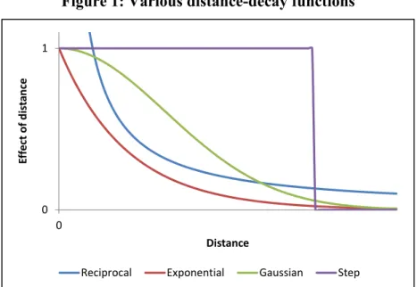
Figure 1: Various distance-decay functions

and k is a constant. Later, the negative exponential function became common (Ingram, 1971). Using this function, distance enters as exp(-λcij), where λ is a constant.

The reciprocal and negative exponential functions can be combined to form the Gaussian (or normal) function. The two former functions have one potentially disadvantageous property (Ingram, 1971). They decline rapidly close to the origin and then level out. The Gaussian function does not have this property but is relatively flat near the origin. The Gaussian function can be modeled as exp(-hcij -k), where both h and k are constants. A very basic method of

representing the distance effect is to use a step function, where distance has no effect until a specific distance at which the effect is infinite. Figure 1 above displays these different forms of curves modeling distance-decay.

4.1 Using accessibility to determine the distance-decay parameter

In an evaluation of different accessibility measures, Song (1996) concludes that the exponential distance-decay function exp(-λ cij) performs best. In the evaluation, he compares

nine different functions using regression analysis and explains population density by accessibility to jobs. In his exercise, Song uses maximum explanatory power as the evaluation criterion. The negative exponential function is arguably the function with the most rigorous theoretical underpinning – random utility theory.

For this reason we use the negative exponential function in our work. We follow Song (1996) to determine the distance-decay parameters for the four major types of retail services: Food, Clothing, Household goods, and Specialized. Statistics Sweden collects data on the level Small Areas for Market Statistics (SAMS-areas). We use the SAMS-areas that are located in the Stockholm functional economic region (FER). The Stockholm FER consists of 36 municipalities and is delineated based on commuting patterns so that the interactions among municipalities and SAMS-areas within the region are relatively large and the interactions with other regions are relatively small. A Swedish municipality is the smallest regional division that has its own administration—the right to collect taxes, and so forth. The SAMS-areas are identified on a

0 1 0 Ef fe ct of dis ta n ce Distance

(12)

municipal sub-division based on electoral districts. There are approximately 9,200 SAMS-areas in Sweden, and 1,275 of these areas are located in the Stockholm FER.

In the empirical sections below, we assume that the location of retail employment is determined by the locus of purchasing power. Retail employment in a SAMS-area is a function of the wages paid to people living there and in neighboring municipalities. The crucial task is to determine the spatial discounting of these neighboring areas. A relatively large distance-decay parameter means that wages made at some distance away do not significantly contribute to the demand for retail services. In contrast, a small distance-decay parameter means that purchasing power does not decay considerably over space.

This relationship can be expressed by the following equation:

(1) , , ,

, denotes employment in SAMS-area r in retail sector s. , is the market potential in

SAMS-area relevant to retail sector , and denotes other characteristics in SAMS-area influencing retail employment. In the empirical application below, we use the Gender composition (the relationship between males and females in each area) and Average age of the population as controls.

The market potential for retail sector s in SAMS-area r is defined as

(2) _, ∑ ∙

is the set of all 1,275 SAMS-areas in the Stockholm FER. Wk is the sum of all wages made by

people living in SAMS-area . drk is the (shortest) distance in meters between SAMS-areas r and k, and is the distance-decay parameter for retail sector . The distance between every pair of areas is calculated based on the location of a centroid of each SAMS-area on a grid.3_{Thus, the}

market potential in an area is a weighted sum of all of the wages made in the Stockholm FER where the weights are determined by the exponential of the distance multiplied by the distance-decay parameter .

Now, we follow an optimization procedure to determine the respective distance-decay parameter for each of the four types of retailing activities. For empirical purposes, Equation (1) can be written (adding an error term) to read:

(3) ln _, ln _, _,

In Equation (3), GC denotes gender composition and AA denotes average age. Equation (3) can be rewritten as:

(4) ln _, ln ∑ ∙ _,

The employment and market potential variables are logged; thus, in the model can be interpreted as an elasticity. The idea is to find the optimal lambdas ( ) in Equation (4) for each retail sector. The optimal lambda is defined as the value where the explanatory power ( ) of the model is maximized. Finding the different lambdas entails determining the -coefficients by OLS while simultaneously optimizing the value of lambda in a non-linear manner. The algorithm we use is the Generalized Reduced Gradient Algorithm (GRG). The results have also been

(13)

obtained by a grid search method. This was accomplished by running numerous OLS regressions while changing by a small amount between each round.

4.1.1 Descriptive statistics and location patterns of retail in the Stockholm region

Table 2 presents descriptive statistics for the four types of retail services under consideration. The table presents statistics where the observational unit is the 1,275 SAMS-areas in the Stockholm FER. The sum column provides the size of the four sectors in terms of total employment in the entire region. The Food retailing sector employs more than 21,000 people, while the Clothing and Specialized sectors employ approximately 12,000 people each, and the Household goods retailing sector employs slightly less than 10,000 people. Although the total number of people employed in Food retailing in total is considerably higher compared to the other three sectors, the maximum number of people employed in an individual SAMS-area is considerably lower. This means that there is a much wider spatial distribution of many stores for this retail service. Another interesting figure is the standard deviation of the Clothing sector, which is considerably higher than it is for the other three types of retail services. This observation implies a higher degree of clustering of this retail service, meaning that there are SAMS-areas with either very few or quite a number of Clothing stores.

Looking at the minimum values, we see that they are zero for each of the retail sector categories, indicating that there are areas with no employment in these sectors. In fact, there are many such areas, as shown in the rightmost column of Table 2, which provides the number of SAMS-areas where each sector has at least one employed person. This means that even for the retail sector present in the most areas (specialized retailing present in 594 out of 1,275 areas), there are still many zero observations. We address this potential problem below.

Next, we observe substantial variation in the two control variables Gender composition and Average age. Gender composition is constructed by recording men as zero and women as one. Thus, 0.08 means that only 8 percent of the residents are female in this area, and 0.75 means that 75 percent are female. The mean is very close to 50 percent, although the standard deviation is relatively low. Average age ranges between 18.8 and 77.5, indicating that areas display age-clustering. However, the more extreme areas are very small in terms of the total population size.

Table 2: Descriptive statistics for the SAMS-areas in the Stockholm region

Min Max Sum Mean Std. Dev. No.

Presence Food 0 561 21,171 16.6 42.68 579 Clothing 0 1,887 12,583 9.87 83.81 396 Household goods 0 1,154 9,740 7.64 45.09 464 Specialized 0 1,217 11,994 9.41 47.2 594 Gender composition 0.08 0.75 - 0.49 0.07 - Average age 18.8 77.5 - 46.44 4.6 - Income 79 49,774,951 - 3,288,752 4,900,185 -

(14)

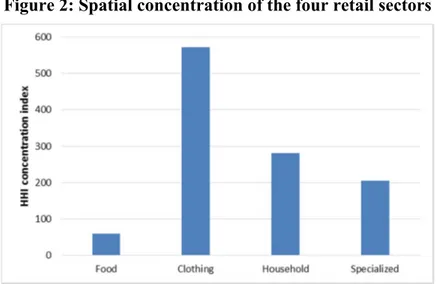
Figure 2: Spatial concentration of the four retail sectors

We calculate the Herfindahl–Hirschman Index4_{(HHI) for each of the four retail sectors}

to more closely examine their spatial distribution. The higher the index, the more concentrated the sector is. The result is displayed in Figure 2 above. We see that clothing retailers are the most spatially concentrated, and the food retailers are the most spatially distributed. The household retailing and specialized retailing lie between these two sectors in terms of spatial concentration.

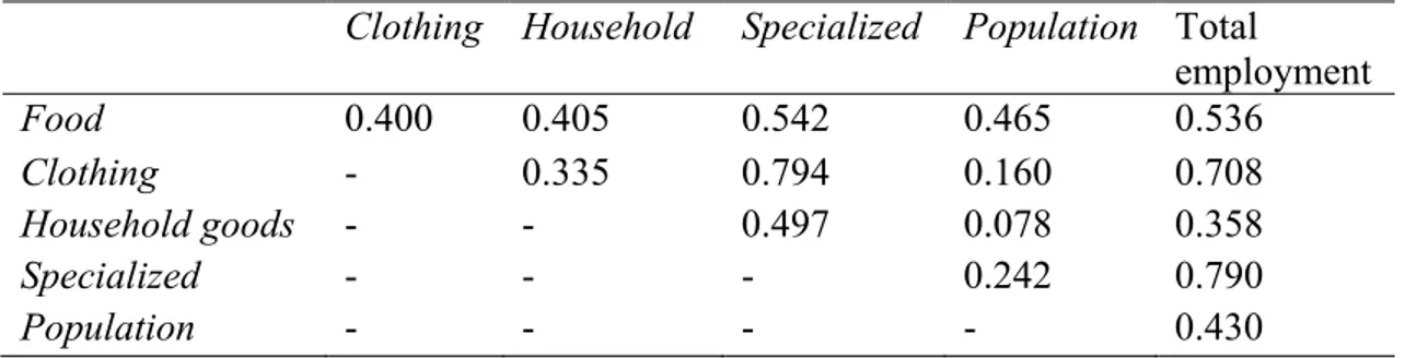
Before we continue to the main analysis, we assess the distribution of the co-location to determine whether or not these retail services are concentrated in the same places. First, we make a preliminary check of the correlation between retail employment and both total employment and population (see Table 3). Specialized retailing is the sector most spatially correlated with total employment, i.e., it has the highest correlation coefficient. A different pattern is observed among correlations with population, for which the highest correlation coefficient belongs to food retailing. Thus, a preliminary analysis indicates that food retailing tends to locate near where people live, whereas specialized and clothing retailers tend to locate near where people work.

The highest correlation coefficient for the spatial correlation among the retail sectors themselves is found between specialized retailers and clothing retailers. The second largest is found between specialized retail and food retailing but this coefficient is substantially smaller than (about 70 percent of) that for specialized and clothing retailers.

The first regression results are given in Table 4 for the simplest model, which has only market potential as an explanatory variable. To avoid potential problems of having too many zero values in the dependent variable, we only run the model on only those SAMS-areas where the respective retail sector is present. Our main interest lies in the variation of the optimized lambda values among the different branches of retail sector. The smallest lambda value is observed for Household goods retailing. This value implies that the distance decay for this particular type of retailing is lower compared to the other three. The largest lambda value is found for Food retailing, indicating that it displays the greatest distance decay of purchasing power. Additionally, the coefficient for the dependence of retail employment on market potential

4_{The HHI is calculated as follows:} _∑ _{, where is the percentage share of total sector employment in area and is}

(15)

Table 3: Correlations between retail employment, population, and total employment

Clothing Household Specialized Population Total

employment Food 0.400 0.405 0.542 0.465 0.536 Clothing - 0.335 0.794 0.160 0.708 Household goods - - 0.497 0.078 0.358 Specialized - - - 0.242 0.790 Population - - - - 0.430

All correlations are statistically significant at the 1 percent level

is approximately 0.3 for the Food, Clothing, and Specialized retailing sectors, indicating that doubling the market potential will increase retail employment in these sectors by approximately 30 percent. The exception is Household goods retailing; this sector has an elasticity of 0.16, indicating that the responsiveness is approximately half as large for this sector compared to the other sectors. Furthermore, the R2_{s- are relatively low. The t-statistics, on the other hand, reveal}

that the dependence on market potential of retail employment location is highly statistically significant.

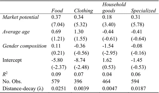
Next, we continue by repeating the estimation and simultaneous optimization by including two more control variables. The variables we introduce in the models of Table 5 are Average age and Gender composition, as introduced above. We can observe a similar trend between the two results. The elasticities with respect to Market potential are similar to those in Table 4. For three sectors the optimized distance-decay parameters are virtually the same between the two tables. The sector that deviates from this pattern is Household goods retailing: its lambda has nearly doubled. This suggests that the distance effect is considerably larger in the more elaborate model. We find the explanation when we look at the two control variables. Average age is statistically insignificant for all four sectors. The gender composition variable is also statistically insignificant, except for the case of Household goods retailing, for which the effect is statistically significant and negative. This suggests that employment in that sector is lower in locations where more women tend to live and higher where more men tend to live.

Table 4: Retail employment location explained by market potential (Model 1)

Food Clothing Household goods Specialized Market potential 0.36 0.31 0.16 0.32 (7.25) (5.14) (3.33) (6.28) Intercept -2.95 -3.59 -0.87 -3.20 (-3.74) (-3.39) (-1.02) (-3.97) R2 _0.08 _0.06 _0.02 _0.06 No. Obs. 579 396 464 594 Distance-decay (λ) 0.0254 0.0037 0.0025 0.0186

(16)

Table 5: Retail employment location explained by market potential, age structure, and gender mix (Model 2)

Food Clothing Household goods Specialized Market potential 0.37 0.34 0.18 0.31 (7.04) (5.32) (3.40) (5.78) Average age 0.69 1.30 -0.44 -0.41 (1.21) (1.55) (-0.61) (-0.64) Gender composition 0.11 -0.36 -1.54 -0.08 (0.21) (-0.56) (-2.95) (-0.16) Intercept -5.80 -8.74 1.62 -1.45 (-2.37) (-2.48) (0.53) (-0.53) R2 _0.09 _0.07 _0.04 _0.06 No. Obs. 579 396 464 594 Distance-decay (λ) 0.0251 0.0039 0.0047 0.0187

Note: t-statistics in parenthesis

Table 6: Retail employment location explained by market potential, age structure, and gender mix (Model 3)

Food Clothing Household goods Specialized Market potential 0.15 0.08 0.06 0.11 (6.40) (4.62) (3.31) (5.13) Average age 0.22 0.28 -0.15 -0.17 (0.88) (1.29) (-0.69) (-0.70) Gender composition 0.13 -0.04 -0.59 -0.05 (0.55) (-0.19) (-3.04) (-0.22) Retail? -2.64 -1.78 -1.92 -1.76 (-48.94) (-37.2) (-42.59) (-34.09) Intercept -0.50 -0.65 1.93 0.73 (-0.47) (-0.70) (2.13) (0.71) R2 _0.70 _0.55 _0.61 _0.54 No. Obs. 1275 1275 1275 1275 Distance-decay (λ) 0.0231 0.0013 0.0024 0.013

Note: t-statistics in parenthesis

As a robustness check, Table 6 presents the model shown in Table 5 but using all observations, including those without a retail presence—all 1,275 observations (SAMs). We introduce a dummy variable that identifies SAMS-areas with no retail employment. This variable takes on the value of one if there is no retail employment and zero otherwise. Note that the elasticities with respect to Market potential are now considerably lower than those in the other two models for all three retail sectors. The other major difference is the size of the R2_{s, which are}

(17)

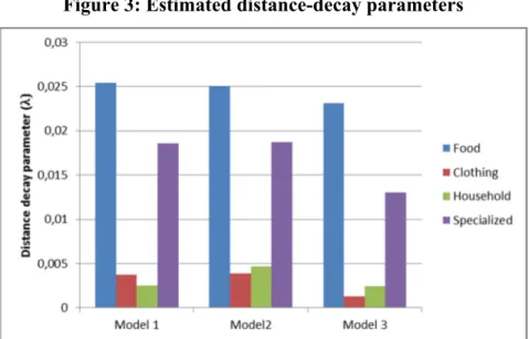
Figure 3: Estimated distance-decay parameters

also considerably higher. This difference is due to the introduced dummy variable Retail, which is statistically significant. This result is expected because so much variation in the dependent variable is explained by the simple presence/nonpresence of any retail employment.

Gender composition’s coefficient is negative and statistically significant for the Household goods retailing sector in this model. The distance-decay parameters are smaller compared to the other estimated models presented in Tables 4 and 5. In Figure 3 below, we collect the results concerning the optimized distance-decay parameters. Models 1, 2, and 3 refer to the results presented in Tables 3, 4, and 5, respectively. The major message as conveyed by Figure 3 is that our results are relatively stable both between and within model specifications.

It may seem unexpected that although the method is implemented to maximize the R2_s,

they remain relatively small for the results presented in Tables 4 and 5 (approximately .10). These relatively small values occur because the models are overly simplified. Although it is safe to argue that Market potential is probably the most important explanatory variable, there are still certain effects that are not counted. For example, a fully specified model should ideally take intervening opportunities into account. In our models, we implicitly assume that consumers go to the nearest shop. We also do not explicitly consider the co-location of several retail activities and related land values. Figure 4 presents the relationship between distance-decay and distance for the different values obtained for retail services. The lambdas used for Figure 4 are those from Model 2. We see that distance decay declines sharply for Food and Specialized retailing, and a lesser attenuation is observed for the Clothing and Household goods retailing sectors. These results confirm the theoretical discussion on distance sensitivity for different types of retail services. These curves, to some extent, display the desire lines discussed by Dicken and Lloyd (1990). Given that the supply occurs where there is sufficient demand for it, we can argue that consumers’ desire to travel further distances for Food and Specialized retailing declines sharply, whereas less sensitivity to distance is observed for retailers selling more durable goods for less frequent purchases in the cases of household and clothing.

In Table 7, we present the figures for the four different accessibility measures obtained for our retail services. The calculations use the different lambda values for each type of retail

(18)

Figure 4: Distance-decay function for four retail sectors (Model 2)

service, as discussed above. Here, we see that the highest average (and median) Market potential is for Clothing retailers, followed by Household goods and Specialized retailers and then Food retailers. We previously mentioned the relationship between the distance-decay function ( values) and the sensitivity to distance for different types of retail services. Based on this argument, it is reasonable to capture the highest accessible market potential for Clothing, where the demand inflows from further distances, as evidenced by the spatial concentration of the sector. Conversely, individuals would most likely shop at the closest Food retailer possible. Comparing the mean values with the respective medians reveals that they are similar, indicating that the variables are not highly skewed.

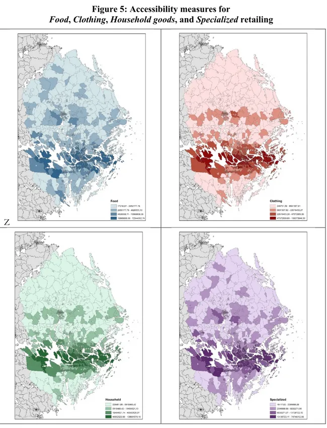
The maps in Figure 5 visualize the distinct market potential measures for the four different types of retailers. In broad strokes, all four maps are rather similar. There is a general pattern of clustering to the center of the Stockholm region, which attenuates as we radiate outward. However, upon further examination, the market potential for Food retailers is more dispersed, and the market potential for Household goods retailers is more clustered.

As a concluding implementation, we use the market potential variables shown in Table 6 and Figure 5 calculated based on the estimated distance-decay parameters for each of the four retail sectors in a simple analysis. We investigate the probability of finding these sectors in different SAMS-areas as dependent on the relevant market potential measure. To this end, we

Table 7: Relevant market potential (accessibility to wages) for the four retail sectors (logged values)

Mean Median Std. Dev. Range Min Max

Food 15.27 15.41 1.22 8.35 9.75 18.1

Clothing 16.69 16.93 1.29 6.44 12.42 18.87

Household goods 16.54 16.78 1.28 6.41 12.34 18.75

(19)

Figure 5: Accessibility measures for

Food, Clothing, Household goods, and Specialized retailing

Z

use a simple logit model relating the probability of retail presence to Market potential. We simply record whether a particular retail sector is present in a SAMS-area and assign the dependent variable 1 if it is and 0 otherwise. For each retail sector, we use the market accessibility corresponding to each unique distance-decay parameter. The fitted value of this

(20)

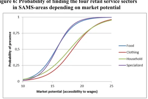
Figure 6: Probability of finding the four retail service sectors in SAMS-areas depending on market potential

logit regression is displayed in Figure 6. The probability of finding a Food or a Specialized store increases sharply at a relatively low value of the Market potential. For the other two sectors (Clothing and Household goods), the probability also increases with increasing Market potential but at a slower rate

The curves in Figure 6 can be interpreted as showing how large Market potential needs to be in order for there to be a 50 percent likelihood of finding a particular retail sector. Conversely, one can consider a particular SAMS-area (with a given market potential) and determine the probability for the presence of each retail sector. Such information can potentially be useful for retailers contemplating establishing a new shop or for a regional policy maker to identify retailing activities that “are missing” or “are at risk of disappearing.”

5. CONCLUDING REMARKS

The relationship between market size and the spatial distribution of retailing has attracted the attention of many researchers, some of which aimed to build models for the identification of market reach for this highly location-dependent economic activity. However, empirical applications of most models have been very challenging because of a lack of data on consumer behavior. In many cases, applications require a researcher to know how many consumers travel how far to patronize a store. In particular, comparison across different branches of the retail sector has been impossible because the data is either only available for a particular type of retailing activity or a particular retail market area. Having limited information on the relationship between potential demand and the market reach of retailing is problematic because an investigation conducted with such data will not yield useful information on spatial continuity, which lies at the heart of the market reach discussion.

If there is a difference in the willingness to travel for different types of shopping trips, the market potential will be different for different parts of the retailing industry. The spatial extent of demand is often operationalized through a distance-decay function in the regional economics literature. In this context, a distance-decay function is an indicator of sensitivity to distance, determining the market reach for an economic activity in question. The purpose of this paper is

(21)

to estimate such distance-decay functions for four different retail sectors in the face of the absence of survey data on consumer behavior. Several retailing activities are nested under four major categories based on their nature and intensity of the interaction they require. These categories are food, clothing, household, and specialized retailing. In the estimation, we use data from the Stockholm FER in Sweden. The unit of observation is the SAMS-areas, with a spatial resolution of 1,275 sub-areas in this region. We use Stockholm as an example because it is the ideal representative market, as all four types of retailing activities are present to a reasonable degree. Following an optimization procedure, we determine four different distance-decay parameters for the four different types of retailing activities in question.

Our findings suggest a higher degree of distance sensitivity to demand for retailers that are selling low-order goods and that rely on frequent interactions with consumers. This type of retailing is also less clustered in space, and the probability of finding such retailing activity is heavily dependent on proximate demand. In contrast, we find a lower distance decay for retailers selling high-order goods (i.e., furniture stores) and a higher degree of clustering of this type of store in space. Both the methodology followed in this paper and its outcome offer an opportunity to (i) create a robust retail categorization, (ii) identify the distance decay for different types of retailing activities, and (iii) operationalize despite the lack of survey data.

REFERENCES

Adler, Thomas and Moshe Ben-Akiva. (1979) “A Theoretical and Empirical Model of Trip Chaining Behavior,” Transportation Research Part B, 13, 243–257.

Alonso, William. (1964) Location and Land Use; Toward a General Theory of Land Rent. Harvard University Press: Cambridge, Massachusetts.

Arentze, Theo A., Harmen Oppewal, and Harry J. Timmermans. (2005) “A Multipurpose Shopping Trip Model to Assess Retail Agglomeration Effects,” Journal of Marketing Research, 42, 109–115.

Batty, Michael. (1971) “Exploratory Calibration of a Retail Location Model Using Search by Golden Section,” Environment and Planning, 3, 411–432.

Batty, Michael and Arild Saether. (1972) “A Note on the Design of Shopping Models,” Journal of the Royal Town Planning Institute, 58, 303–306.

Becker, Gary S. (1965) “A Theory of the Allocation of Time,” Economic Journal, 75, 493–517. Ben-Akiva, Moshe and Steven R. Lerman. (1985) Discrete Choice Analysis: Theory and

Application to Travel Demand. MIT Press: Cambridge, Massachusetts.

Berry, Brian J. and William L. Garrison. (1958) “Recent Developments of Central Place Theory,” Papers in Regional Science, 4, 107–120.

Brown, Stephen. (1992) “The Wheel of Retail Gravitation,” Environment and Planning A, 24, 1409–1429.

Bunch, David. S., Mark Bradley, Thomas F. Golob, Ryuichi Kitamura, and Gareth P. Occhiuzzo. (1993) “Demand for Clean-Fuel Vehicles in California: A Discrete-Choice Stated Preference Pilot Project,” Transportation Research A, 27, 237–253.

(22)

Burkey, Jake and Thomas R. Harris. (2003) “Modeling a Share or Proportion with Logit or Tobit: The Effect of Outcommuting on Retail Sales Leakages,” Review of Regional Studies, 33, 328–342.

Cadwallader, Martin T. (1996) Urban Geography: An Analytical Approach. Prentice Hall: Upper Saddle River, New Jersey.

Carrothers, Gerald A. (1956) “An Historical Bedew of the Gravity and Potential Concepts of Human Interaction,” Journal of the American Institute of Planners, 22, 94–102.

Christaller, Walter. (1933) Die zentralen Orte in Süddeutschland. Gustav Fisher: Jena.

Clark, William A. V. (1968) “Consumer Travel Patterns and the Concept of Range,” Annals of the Association of American Geographers, 58, 386–396.

Converse, Paul D. (1943) A Study of Retail Trade Areas in East Central Illinois. University of Illinois.

_____. (1949) “New Laws of Retail Gravitation,” Journal of Marketing, 14, 379–384. Curry, Les. (1972) “A Spatial Analysis of Gravity Flows. Regional Studies,” 6, 131–147.

Damm, David and Steven R. Lerman. (1981) “A Theory of Activity Scheduling Behavior,” Environment and Planning A, 13, 703–718.

Dicken, Peter, and Peter E. Lloyd. (1990) Location in Space: Theoretical Perspectives in Economic Geography. Harper & Row: New York.

Eaton, Curtis B. and Richard G. Lipsey. (1975) “The Principle of Minimum Differentiation Reconsidered: Some New Developments in the Theory of Spatial Competition,” Review of Economic Studies, 42, 27–49.

Fotheringham, Stewart A. (1983a) “A New Set of Spatial-Interaction Models: The Theory of Competing Destinations,” Environment and Planning A, 15, 15–36.

_____. (1983b) “Some Theoretical Aspects of Destination Choice and Their Relevance to Production-Constrained Gravity Models,” Environment and Planning A, 15, 1121–1132. _____. (1984) “Spatial Flows and Spatial Patterns,” Environment and Planning A, 16, 529–543. _____. (1988) “Consumer Store Choice and Choice Set Definition,” Marketing Science, 7, 299–

310.

Fotheringham, Stewart A. and Morton E. O'Kelly. (1989) Spatial Interaction Models: Formulations and Applications. Kluwer Academic: Dordrecht.

Fotheringham, Stewart A. and Michael J. Webber. (1980) “Spatial Structure and the Parameters of Spatial Interaction Models,” Geographical Analysis, 12, 33–46.

Gärling, Tommy, Mei-Po Kwan, and Reginald. G. Golledge. (1994) “Computational-Process Modelling of Household Activity Scheduling,” Transportation Research B, 28, 355–364. Getis, Arthur and Judith Getis. (1966) “Christaller's Central Place Theory,” Journal of

Geography, 65, 220–226.

Ghosh, Avijit and Sara L. McLafferty. (1987) Location Strategies for Retail and Service Firms. Lexington Books: Lexington, Massachusetts.

(23)

Goldstucker, Jac L., Danny N. Bellenger, Thomas J. Stanley, and Ruth L. Otte. (1978) New Developments in Retail Trading Area Analysis and Site Selection. Publishing Services Division, College of Business Administration, Georgia State University.

Golledge, Reginald G. and Robert. J. Stimson. (1997) Spatial Behavior: A Geographic Perspective. Guilford: New York.

Golledge, Reginald G., Gerard Rushton, and William A. Clark. (1966) “Some Spatial Characteristics of Iowa's Dispersed Farm Population and Their Implications for the Grouping of Central Place Functions,” Economic Geography, 42, 261–272.

Gruidl, John and Dimitri Andrianacos. (1994) “Determinants of Rural Retail Trade: A Case Study of Illinois,” Review of Regional Studies 24, 103–118.

Haining, Robert. (1984) “Testing a Spatial Interacting-Markets Hypothesis,” Review of Economics and Statistics, 66, 576–583.

Hansen, Walter G. (1959) “How Accessibility Shapes Land Use,” Journal of the American Institute of Planners, 25, 73–76.

Hanson, Susan and James O. Huff. (1988) Repetition and Day-To-Day Variability in Individual Travel Patterns: Implications for Classification. Croom Helm: London.

_____. (1986) “Classification Issues in the Analysis of Complex Travel Behavior,” Transportation, 13, 271–293.

Haynes, Kingsley E. and Stewart A. Fotheringham. (1984) Gravity and Spatial Interaction Models Vol. 2. Sage Publications: Beverly Hills, California.

Hotelling, Harold. (1929) “Stability in Competition,” Economic Journal, 39, 41–57.

Huff, David L. (1964) “Defining and Estimating a Trading Area,” Journal of Marketing, 28, 34– 38.

Huff, David L. and George F. Jenks. (1968) “A Graphic Interpretation of the Friction of Distance in Gravity Models,” Annals of the Association of American Geographers, 58, 814–824. Ingene, Charles A. and Eden S. H. Yu. (1981) “Determinants of Retail Sales in SMSAs,”

Regional Science and Urban Economics, 11 529–547.

Ingram, David. R. (1971) “The Concept of Accessibility: A Search for an Operational Form,” Regional Studies, 5, 101–107.

Johnston, Robert J. (1976) “On Regression Coefficients in Comparative Studies of the ‘Frictions of Distance’,” Tijdschrift Voor Economische En Sociale Geografie, 67, 15–28.

Kitamura, Ryuichi, Kazuo Nishii, and Konstadinos Goulias. (1990) “Trip Chaining Behavior by Central City Commuters: A Causal Analysis of Time-Space Constraints,” Developments in Dynamic and Activity-Based Approaches to Travel Analysis, 145–170.

Kivell, Phillip T. and Gareth Shaw. (1980) “The Study of Retail Location,” in John Dawson (ed.), Retail Geography. RLE Retailing and Distribution: New York.

Lakshmanan, T. R. and Walter G. Hansen. (1965) “A Retail Market Potential Model,” Journal of the American Institute of Planners, 31, 134–143.

(24)

Larsson, Johan P. and Özge Öner. (2014) “Location and Co-Location in Retail: A Probabilistic Approach Using Geo-Coded Data For Metropolitan Retail Markets,” Annals of Regional Science, 52, 385–408.

Lösch, August. (1940) Die Räumliche Ordnung der Wirtschaf, trans. Yale University Press: New Haven, Connecticut.

Luce, Duncan R. (1959) Individual Choice Behavior: A Theoretical Analysis. Dover Publication: New York.

Mayo, Edward J., Lance P. Jarvis, and James A. Xander. (1988) “Beyond the Gravity Model,” Journal of the Academy of Marketing Science, 16, 23–29.

McGoldrick, Peter J. (1990) Retail Marketing. McGraw-Hill: Maidenhead.

Mulligan, Gordon F. (2012) Stochastic Shopping and Consumer Heterogeneity. Studies in Regional Science, 42, 93–107.

Mulligan, Gordon F., Marian L. Wallace, and David A. Plane. (1985) “A General Model for Estimating the Number of Tertiary Establishments in Communities: An Arizona Perspective,” Social Science Journal, 22, 77–93.

Newmark, Gregory L. and Pnina O. Plaut. (2005) “Shopping Trip-Chaining Behavior at Malls in a Transitional Economy,” Transportation Research Record: Journal of the Transportation Research Board, 1939, 174–183.

O'Kelly, Morton E. (1981) “A Model of the Demand For Retail Facilities, Incorporating Multistop, Multipurpose Trips,” Geographical Analysis, 13, 134–148.

_____. (1983) “Impacts of Multistop, Multipurpose Trips on Retail Distributions,” Urban Geography, 4, 173–190.

Parr, John B., and Kenneth G. Denike. (1970) “Theoretical Problems in Central Place Analysis,” Economic Geography, 44, 568–586.

Prelec, Dražen. (1982) “Matching, Maximizing, and the Hyperbolic Reinforcement Feedback Function,” Psychological Review, 89, 189–230.

Reilly, William J. (1929) Methods for the Study of Retail Relationship. University of Texas Bulletin.

_____. (1931) The Law of Retail Gravitation. Pillsbury Publishers: New York.

_____. (1953) The Law of Retail Gravitation, 2nd_{ed. Pillsbury Publishers: New York.}

Rouse, William J. (1953) “Estimating Productivity for Planned Regional Shopping Centers,” Urban Land, 12, 1–6.

Song, Shunfeng. (1996) “Some Tests of Alternative Accessibility Measures: A Population Density Approach,” Land Economics, 72, 474–482.

Stewart, John Q. (1948) Demographic Gravitation: Evidence and Applications. Beacon House: Boston, Massachusetts.

Thill, Jean-Claude and Isabelle Thomas. (1987) “Toward Conceptualizing Trip‐Chaining Behavior: A Review,” Geographical Analysis, 19, 1–17.