NEAR-INFRARED SPECTROSCOPY
FOR REFUSE DERIVED FUEL
CHARACTERIZATION
Classification of waste material components using hyperspectral imaging and
feasibility study of inorganic chlorine content quantification
MARTIN ŠEVČÍK
School of Business, Society and Engineering Course: Degree project in energy engineering Course code: ERA 403
Credits: 30 hp
Program: Sustainable energy systems
Supervisor: Jan Skvaril Examiner: Xin Zhao
Customer: MDH, Mälarenergi AB, FUDIPO Date: 2019-01-14
Email: msk17005@student.mdh.se mrt.sevcik@gmail.com
i
ABSTRACT
This degree project focused on examining new possible application of near-infrared (NIR) spectroscopy for quantitative and qualitative characterization of refuse derived fuel (RDF). Particularly, two possible applications were examined as part of the project. Firstly, use of NIR hyperspectral imaging for classification of common materials present in RDF. The classification was studied on artificial mixtures of materials commonly present in municipal solid waste and RDF. Data from hyperspectral camera was used as an input for machine learning models to train them, validate them, and test them. Three classification machine learning models were used in the project; partial least-square discriminant analysis (PLS-DA), support vector machine (SVM), and radial basis neural network (RBNN). Best results for classifying the materials into 11 distinct classes were reached for SVM (accuracy 94%), even though its high computational cost makes it not very suitable for real-time deployment. Second best result was reached for RBNN (91%) and the lowest accuracy was recorded for PLS-DA model (88%). On the other hand, the PLS-DA model was the fastest, being 10 times faster than the RBNN and 100 times faster than the SVM. NIR spectroscopy was concluded as a suitable method for identification of most common materials in RDF mix, except for incombustible materials like glass, metals, or ceramics. The second part of the project uncovered a potential in using NIR spectroscopy for identification of inorganic chlorine content in RDF. Experiments were performed on samples of textile impregnated with a water solution of kitchen salt representing NaCl as inorganic chlorine source. Results showed that contents of 0.2-1 wt.% of salt can be identified in absorbance spectra of the samples.
Limitation appeared to be water content of the examined samples, as with too large amount of water in the sample, the influence of salt on NIR absorbance spectrum of water was too small to be recognized.
Keywords: near-infrared spectroscopy, NIR, municipal solid waste, MSW, refuse derived
fuel, RDF, classification, chemometrics, machine learning, artificial neural network, radial basis neural network, high-temperature corrosion, chlorine, waste to energy
ii
PREFACE
This degree project was part of master’s level studies of program Sustainable energy systems at Mälardalen University in Västerås, Sweden. The topic of this study was initiated together with Jan Skvaril, Assistant Professor in Energy Engineering at Mälardalen University, who was also the supervisor of the project.
The project was financially supported by Mälarenergi AB and FUDIPO research project. FUDIPO, or Future Directions of Production Planning and Optimized Energy – and Process Industries, is an EU funded project focused on developing and testing new methods of mathematical modeling and simulation for energy and process industry. These new methods should contribute to the improvement of current processes and development of new
production system solutions.
I would like to thank Jan Skvaril as my supervisor for his professional guidance and support. His wide range of experience in the field of NIR spectroscopy contributed a lot to this work. Secondly, I want to thank Elena Tomás-Aparicio as my external supervisor and
representative of Mälarenergi AB and FUDIPO project. She contributed to this work through her experience with RDF and operation of waste-to-energy thermal power plants.
I would also like to thank Xin Zhao, Assistant Professor in Energy Engineering at Mälardalen University and examiner of this work, for all his feedback that helped to elevate the quality of this work.
Finally, I would like to thank my family for their continuous support and love throughout my whole studies.
Västerås, January 2019
iii
SUMMARY
Modern society produces large amounts of waste and a need for efficient and
environmentally friendly utilization of the waste increases. Energy recovery should be
preferred over landfilling due to its environmental benefits and due to the increasing number of countries introducing landfill bans. But using municipal solid waste as a fuel, often pre-processed into refuse derived fuel (RDF), comes with many challenges. For example, very high variability in composition and highly corrosive effects on boilers. Therefore, fast and reliable technologies are researched to provide needed information about the fuel to waste-to-energy plant operators.
One of the technologies that present a good potential for such application is near-infrared (NIR) spectroscopy. It is based on observation of how certain material absorbs light at certain wavelengths of NIR spectrum (wavelengths 700-2500 nm). This technology has already been successfully applied in the food and pharmaceutic industry, or in biomass thermal conversion processes and sorting of plastics. It was also proven to work for most of the common
materials in the municipal solid waste, therefore it should be possible to develop a model that would be capable of telling these materials apart. Information from the NIR absorbance spectra is analyzed using chemometric techniques, which is an approach combining data analysis and machine learning for quantitative and qualitative characterization of materials. Three machine learning models were developed for a classification of materials into 11 different classes. It was partial least-square discriminant analysis (PLS-DA), support vector machine (SVM), and radial basis neural network (RBNN). The classification was performed on hyperspectral images of the materials placed on a background similar to a conveyor belt. The hyperspectral image is 𝑀 × 𝑁 × 𝑊 block of data created from stacking images of 𝑀 × 𝑁 pixels captured at 𝑊 different light wavelengths. The classification models differ in the way they conduct classification, in how complex they are, and how high computational cost they have. They were developed and tested using artificial waste mixtures created from typical household items, which compared to real waste allowed more control over the composition of the mixtures and was favored for hygienic reasons. Evaluation of classification accuracy was done through internal holdout validation and external sample validation.
Best performing model was SVM, reaching up to 94% accuracy of classification. But this model had very high computational cost and was therefore considered as not suitable for potential application for real-time classification of materials on a conveyor belt. Second best results were reached for the RBNN model with 91% classification accuracy, which is
approximately 10 times faster than the SVM model. Lowest accuracy of 88% was reached with PLS-DA model that was also least complex and approximately 100 times faster than the SVM model. Accuracies and speed of all models could also be increased by decreasing
resolution of the hyperspectral image that was used as an input for classification. Results also show that the models could identify most of the material present in the MSW very well, except incombustible materials. These materials, like metal, ceramics, and glass, don’t have a specific absorbance profile in the NIR spectrum, therefore their classification was
iv
The second part of the project was focused on identification of inorganic chlorine content in RDF. A number of studies has identified inorganic chlorine represented by NaCl and KCl as the most problematic component in RDF due to its severe high-temperature corrosive effect. Melted (Na, K)Cl reacts in presence of oxide with an oxidized surface layer of boiler’s
superheaters that serves as protection against corrosion. This reaction leads to destruction of the protective layer of oxides, high corrosion rate, and therefore increased maintenance costs or even unplanned shutdowns of the boiler.
Studies from the food industry have shown that it is possible to identify the content of NaCl, which is the main representative of inorganic chlorine in MSW, through its influence on the absorbance of water in the NIR spectrum. The influence can be observed as scaling and shifting of peaks in absorbance spectra of water. Presence of inorganic chlorine in RDF was simulated by impregnating textile samples with a mixture of water and kitchen salt (NaCl). The salt content ranged between 0.2-1 wt.% of the dry base material and a water content between 6-120 wt.% of the dry base material, which are typical values for RDF.
The relation between NIR absorbance spectra and salt content was examined using partial least-square regression, which is a common method in NIR spectroscopy. Results of this experiment showed that the effect of NaCl on water could be observed even for these low concentrations of salt, but only for lower concentrations of water in the samples. As the water concentration got higher (60-120 wt.%), the ratio of salt/water got probably too low to have a recognizable effect on water’s absorbance.
Overall, it was concluded that it should be possible to develop a method combining NIR spectroscopy and machine learning that would be capable of recognizing main components of the real MSW and RDF in the real-time. Such method could improve operation of waste to energy plants and be used for automated sorting of MSW. NIR spectroscopy also shows potential to be used as a fast, non-destructive tool for identification of inorganic chlorine content in RDF.
v
TABLE OF CONTENT
1 INTRODUCTION ...1
1.1 Background ... 1
1.1.1 Importance of energy recovery ... 1
1.1.2 Solid waste as a fuel ... 2
1.1.3 Spectroscopy as a tool for characterization ... 3
1.1.4 Problem of chlorine content... 3
1.2 Purpose ... 4
1.3 Research questions ... 4
1.4 Scope and delimitations ... 5
2 LITERATURE REVIEW ...6
2.1 NIR spectroscopy ... 6
2.1.1 Basic principles ... 6
2.1.2 Hyperspectral imaging ... 8
2.2 Chemometrics and machine learning ...10
2.2.1 Data pre-processing ...10
2.2.2 Basics of machine learning ...11
2.2.3 Quantitative methods ...11
2.2.4 Qualitative methods ...13
2.2.5 Workflow of data handling ...15
2.3 Applications of NIR spectroscopy ...16
2.4 Waste and refuse derived fuel ...18
2.4.1 Waste-to-energy combustion plant ...18
2.4.2 Preparation of refuse derived fuel ...19
2.4.3 Emerging methods for composition characterization ...19
2.4.4 Common components ...20
2.5 Problems caused by presence of chlorine ...21
2.5.1 High-temperature corrosion...22
2.5.2 Prevention of high-temperature corrosion ...23
2.5.3 Sources of chlorine ...24
vi
3 METHOD ... 27
3.1 Experiment setup ...27
3.2 Samples ...28
3.3 Data and chemometrics ...31
3.3.1 Camera calibration and faulty data elimination ...31
3.3.2 Pre-processing of data ...33
3.3.3 Training and validation ...34
3.3.4 External validation of the model ...35
3.3.5 Measures of model’s performance ...35
3.4 Experiment flowcharts ...37
3.5 Spectroscopy background justification ...38
3.6 Software ...38
4 RESULTS ... 39
4.1 Classification of waste components ...39
4.1.1 Spectral profiles of materials ...39
4.1.2 Influence of pre-processing on accuracy ...41
4.1.3 Class confusion ...42
4.1.4 Merging material classes ...42
4.1.5 External validation ...46
4.1.6 Most influential bands for classification ...51
4.2 Identification of inorganic chlorine content ...52
4.2.1 Data combination and influence of pre-processing ...53
4.2.2 Influence of water content ...53
4.2.3 Closer analysis of spectral profiles ...55
4.2.4 Water evaporation ...56
5 DISCUSSION... 57
5.1 Classification models ...57
5.1.1 Performance of models ...57
5.1.2 Recognized materials and confusions ...59
5.1.3 Spectroscopy background justification ...59
vii
5.2 Identification of inorganic chlorine content ...61
5.3 Reflection on social, economic and environmental aspects of the work ...62
6 CONCLUSIONS ... 63
FUTURE WORK ... 64
viii
LIST OF FIGURES
Figure 1: Waste management hierarchy based on Waste Framework Directive 2008/98/EC .. 1
Figure 2: General principle of absorption spectroscopy ... 7
Figure 3: Principle of diffuse reflection ... 7
Figure 4: Example of hyperspectral image (hypercube) ... 9
Figure 5: Types of scanning methods in hyperspectral imaging ... 9
Figure 6: Mapping by PLS and PCA ...12
Figure 7: Mapping by PLS and PCA with random noise ...12
Figure 8: Basic principle of PLS-DA and maximizing separability... 13
Figure 9: Basic principle of support vector machine ...14
Figure 10: Basic principle of radial basis function neural network ...14
Figure 11: General workflow of chemometric process ... 15
Figure 12: Circulating fluidized bed boiler at Västerås (block 6) – scheme created and used with permission from Valmet ... 18
Figure 13: Comparison of MSW and RDF composition – data retrieved from Montejo et al. (2011) ...19
Figure 14: Simplified scheme of high temperature corrosion due to organic chlorine ... 23
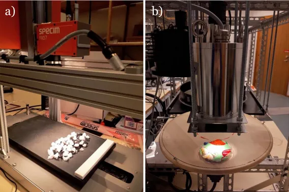
Figure 15: Schematic setup for measurements with hyperspectral camera ... 27
Figure 16: Experimental setups – a) setup with hyperspectral camera, b) setup with FT-NIR sensor ... 28
Figure 17: a) Training mix of polystyrene samples b) External validation mix of polystyrene samples ... 29
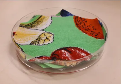
Figure 18: Sample for experiment with NaCl content... 30
Figure 19: Dependency of absorbance spectra on number of textile layers... 31
Figure 20: Spectral profiles of white and dark references (reflectance is expressed in an unspecified signal intensity unit) ... 32
Figure 21: Signal-to-noise profile ... 33
Figure 22: Flowchart of experiment process for classification model development ... 37
Figure 23: Flowchart of experiment process for inorganic chlorine identification ... 38
Figure 24: Relative absorbance spectra of plastics ... 39
Figure 25: Relative absorbance spectra of paper materials ... 40
Figure 26: Relative absorbance spectra of incombustible materials ... 40
Figure 27: Relative absorbance spectra of other materials ...41
Figure 28: Influence of class merging on accuracy ... 43
Figure 29: Classification of testing image by RBNN (first part) ... 47
Figure 30: Classification of testing image by RBNN (second part) ... 47
Figure 31: Classification of testing image by PLS-DA ... 48
Figure 32: Classification of testing image by SVM ... 48
Figure 33: Regression coefficients of PLS-DA model for plastics ... 51
Figure 34: Regression coefficients of PLS-DA model for remaining classes ... 52
Figure 35: Acquired absorbance spectra for various moisture contents (wt.% of dry sample)52 Figure 36: Results of regression for preprocessing by SGF and MSC ... 54
Figure 37: Prediction of salt content depending on water content ... 54
ix
Figure 39: Zoomed in region of spectra for samples with 12 wt.% water content ... 55
Figure 40: Zoomed in region of spectra for samples with 12 wt.% water content ... 56
LIST OF TABLES
Table 1: Common components of RDF and MSW ... 20Table 2: Order of total chlorine content value for waste fractions [wt.% of dry component] . 25 Table 3: List of used samples ... 28
Table 4: Impregnation of samples with salt and water ... 30
Table 5: Evaluation of class prediction ... 36
Table 6: Accuracy of classification models depending on pre-processing ...41
Table 7: Accuracy of classification models depending on pre-processing (after class merging) ... 43
Table 7: Detailed classification results for 18 classes ... 44
Table 8: Detailed classification results for 11 classes ... 45
Table 10: External validation results (11 material classes) ... 46
Table 11: Classification speed of models under specific conditions ... 49
Table 12: Results of classification after resolution decrease ... 49
Table 13: Detailed external validation results for 11 classes ... 50
Table 14: Combining data for samples with various moisture content (wt.% of dry basis) .... 53
NOMENCLATURE
Symbol Description Unit
𝐴𝑅 Relative absorbance [-] 𝑐 Classification speed [px/s] 𝐼 Final relative diffuse reflectance [-] 𝐼0 Light intensity detected by sensor [cd] 𝐼𝐵 Light intensity detected for dark ref. [cd] 𝐼𝐷 Light intensity reflected to sensor [cd] 𝐼𝑅 Relative diffuse reflectance [-] 𝐼𝑆 Light intensity of source [cd] 𝐼𝑊 Light intensity detected for white ref. [cd]
x
Symbol Description Unit
𝑆𝑇𝑁 Signal-to-noise ratio [dB] 𝑣 Speed of conveyor belt [m/s]
𝑣̃ Wavenumber [cm-1]
𝑊 Width of linear field of view [m]
𝜆 Wavelength [nm]
ABBREVIATIONS
Abbreviation DescriptionANN Artificial Neural Network CFB Circulating fluidized bed EU European Union
FT-NIR Fourier transform NIR HDPE High-density polyethylene LDPE Low-density polyethylene LV Latent Variable
MIR Mid-infrared
MSC Multiplicative Scatter Correction MSW Municipal Solid Waste
NIR Near-infrared
NIR-HSI Near-infrared Hyperspectral Imaging PC Principal Component
PCA Principal Component Analysis PE Polyethylene
PET Polyethylene terephthalate PLS Partial Least-squares
PLS-DA Partial Least-squares Discriminant Analysis PLS-R Partial Least-squares Regression
PP Polypropylene PS Polystyrene PU Polyurethane PV Prediction Variable
xi
Abbreviation Description
PVC Polyvinyl chloride
RBNN Radial Basis Neural Network RC Regression Coefficient RDF Refuse Derived Fuel RV Response Variable
SGD’ Savitzky-Golay filter 1st derivative
SGD’’ Savitzky-Golay filter 2nd derivative
SGF Savitzky-Golay Filter SNV Standard Normal Variance SRF Solid Recovered Fuel SVM Support Vector Machine TCC Total Chlorine Content UV Ultraviolet
1
1
INTRODUCTION
The report is a product of research in the fields of spectroscopic analysis of materials and waste to energy (W2E). The primary focus of the study is to examine the possibilities of using near-infrared (NIR) spectroscopic analysis to characterize individual components of refuse derived fuel (RDF) and identify a content of inorganic chlorine in the material stream. The work was conducted as part of FUDIPO project funded by European Commission. The project focuses on optimization and control techniques in industrial processes. Support for the work came also from Mälarenergi AB, a provider of electricity and district heating in the Mälardalen region, and owner of waste combustion power plant in Västerås, Sweden.
1.1 Background
Modern societies all over the world produce large amounts of waste in various forms. With an increasing world population and increasing economic strength of nations, the amount of waste is expected to increase in the following decades. Effects of this are already visible in our oceans polluted with tonnes of waste. Therefore, sustainable waste management approach is needed to solve this environmental threat (Hoornweg et al., 2013).
1.1.1 Importance of energy recovery
As a response to the problem, European Parliament and Council released Waste Framework Directive 2008/98/EC (European Parliament and of the Council, 2008) that provides basic concepts for waste management that should be implemented by EU member states. One of the key parts of the directive is the waste management hierarchy that sets the following priority order:
Figure 1: Waste management hierarchy based on the Waste Framework Directive 2008/98/EC
The approach was validated by various studies (Eriksson et al., 2005, Finnveden et al., 2005). These studies analyzed individual levels of the hierarchy from an environmental point of view and concluded that recycling should indeed be preferred over energy recovery over
2
landfilling. In Sweden, the approach is embraced by legislation valid since the year 2000 that introduces a tax on all landfilled waste. Later in 2002 it was expanded by a ban on landfilling combustible waste and in 2005 by the ban on landfilling organic waste (Eriksson et al., 2005).
Waste to energy (W2E) is a way to utilize energy content in the waste streams. It can be done in various ways, with two main paths being Biochemical energy conversion pathway (e.g. digestion) and Thermochemical conversion pathway (combustion, pyrolysis, and
gasification). When comparing these methods from an environmental point of view, the results of individual studies vary. Dong et al. (2018) concluded that combustion is in favor over pyrolysis and gasification mainly thanks to being mature and well-developed
technology. For organic waste, Fruergaard and Astrup (2011) concluded that incineration is the preferred option over anaerobic digestion because of challenges with digestate utilization. On the other hand, Arafat et al. (2015) suggest that anaerobic digestion and gasification should be preferred over other methods due to overall lower environmental impacts. One of the reasons for these differences is heterogeneity of the waste composition as various
components are suitable for various processes and methods (Arafat et al., 2015, Gunamantha and Sarto, 2012).
1.1.2 Solid waste as a fuel
Municipal solid waste (MSW) contains a lot of incombustible components and has a high moisture content, hence its caloric value is very low. Therefore, processing of MSW is applied to derive a stream with higher caloric value. Such stream is called refuse derived fuel (RDF) (Thorin et al., 2011). It consists mainly of paper, cardboard, plastics, and textiles, but can also contain a larger fraction of food waste, garden waste and wood (Gallardo et al., 2014,
Haydary, 2016, Sarc and Lorber, 2013).
Same as for MSW, one of the key challenges connected to the use of RDF is its heterogeneity and variance in composition. Therefore, reliable and fast characterization of RDF stream is needed. Main properties are caloric value, moisture content, ash content, chlorine content and content of heavy metals (Bessi et al., 2016, Gallardo et al., 2014, Rotter et al., 2011). Generally, RDF itself does not have to comply with any standards for these characteristics. It imposes a challenge for creating a market for RDF because there is no standard that could guarantee the fuel quality. For this reason, a subcategory of solid recovered fuel (SRF) was introduced. SRF must comply with a standard that defines its properties based on its net caloric value, chlorine content and mercury content, which are defined by European standard EN 15359:2011 (European Committee for Standardization, 2011).
The standard also defines sampling and testing methods that must be used to assess the quality of RDF. These methods rely on the extraction of representative samples of an RDF stream. The sample size is based on statistical assumptions that should cover variability in the composition of the stream. Quality tests of these samples are then based on chemical and thermal procedures performed in a laboratory (Rotter et al., 2011, Schwarzböck et al., 2016). As highlighted by Rotter et al. (2011), these methods require a lot of time to be performed, a large amount of laboratory equipment, they are financially demanding, and are not suitable
3
for continuous characterization of the waste material stream. Therefore, new and more effective methods are researched to substitute or support the current standardized ones.
1.1.3 Spectroscopy as a tool for characterization
An interesting new method that can be used for more effective characterization of RDF is spectroscopic analysis, particularly analysis in near-infrared (NIR) part of light spectrum. The method is currently being widely adopted in the pharmaceutical industry (Reich, 2005) and is gaining popularity in the food industry (Wu and Sun, 2013). Also, applications in the field of energy conversion have started to appear in recent years. Skvaril et al. (2017b) provided a complex study of the possible use of NIR spectroscopy in biomass energy conversion process. Wang et al. (2014) used a similar approach to determine properties of coal.
The method was already proven to be working for identification of biomass properties (Skvaril et al., 2017a), identification of various plastics and their sorting (Serranti et al., 2011), characterization of textiles (Cleve et al., 2000) and for identification of paper and cardboard (Tatzer et al., 2005). As these are major components of RDF, it should be possible to develop a model for real-time identification of individual components of the RDF stream and enable its continuous characterization. It would enable operators of thermal power plants using RDF to acquire better knowledge about the fuel and observe possible variations of its properties for process optimization. The real-time character of the data could also be used in earlier stages of the fuel preparation process, for example for sorting, drying and better control over them.
The possibility was already addressed by Dahl (2018) in his thesis on a determination of share of plastics in RDF, and by Hedlund (2018) for a determination of glass content in RDF. In case of plastics content, the precision of 𝑅2= 0.8 and RMSE = 0.09 was reached, whereas for determination of glass content, NIR spectroscopy was not recommended as fa easible option due to its low accuracy.
There is also an industrial solution available on the market (LLA Instruments GmbH & Co. KG). The system uses NIR spectroscopy to determine heating value, moisture content and a chlorine content of RDF. The company also offers solutions for individual plastic sorting, paper sorting, and food sorting. Unfortunately, there are no details available on the used technology and achieved accuracies.
1.1.4 Problem of chlorine content
One of the key properties of RDF is its chlorine content. It has high corrosive effects and causes ash fouling on the heat exchange surfaces, which leads to increased maintenance costs and decreased efficiency (Ma et al., 2010, Silva et al., 2014). The high content of chlorine in the fuel is generally one of the main reasons for the low efficiency of W2E plants (Hunsinger and Andersson, 2014, Sudo et al., 2015). It is because boilers use low-temperature
4
Because of this, W2E plants generally reach an efficiency of only between 15-20% for electricity generation.
As Silva et al. (2014) highlights, chlorine behavior depends on the type of chlorine present in RDF (organic or inorganic) and its amount is dependent on RDF’s composition. Inorganic chlorine comes mainly from the biological fraction of RDF and from food packaging, whereas organic chlorine originates mainly in synthetic organic polymers such as PVC. Therefore, the efficient characterization of RDF’s composition could help to identify main sources of
chlorine-related corrosion and enable subsequent actions. If it was possible to efficiently decrease the corrosive effects of flue gases in W2E plants due to chlorine, their efficiency of electricity generation could be significantly increased. It is because corrosion rates increase with temperature. Therefore, with a lower intensity of chlorine-related corrosion, boilers could be designed for the higher temperature of the output steam, which would lead to higher efficiency of the Rankine cycle (Hunsinger and Andersson, 2014).
1.2 Purpose
The goal of the study is to find out if it is possible to develop a computer model using data from NIR hyperspectral imaging (NIR-HSI) for classifying the wide range of various
materials contained in RDF stream in the real-time. Compared to other research in the field, the project aims to use a single model for classification of all main materials in RDF instead of focusing only on certain material categories. It also examines use of machine learning models that are less common in spectroscopy for energy conversion field. This makes the project unique. If such model would be proved to work, findings of the study could be used to develop a system for automated material sorting or identification of fossil share in the
material stream.
The second part of the project is dedicated to chlorine in RDF. Based on the literature study, it should be identified what type of chlorine (organic or inorganic) in the waste material is more important for corrosive behavior. After that, it will be tested whether NIR spectroscopy might be a feasible method to determine the amount of the chosen type of chlorine in RDF, or not. This type of research has not yet been conducted in the connection to the waste-to-energy field. Results of the feasibility study should serve as a starting point for possible further research of the topic.
1.3 Research questions
The project will address the following research questions;
1. Is it possible to develop a real-time classification model for all typical material in MSW and RDF stream, and what materials can be recognized by NIR spectroscopy with high accuracy depending on the used machine learning model? How can the accuracy be further increased?
5
2. What accuracy does NIR spectroscopy combined with analytical computer models reach for determination of harmful inorganic chlorine content in representative samples of waste material?
1.4 Scope and delimitations
Overall, the study is focused on testing earlier proposed ideas and concepts (chapters 1.2 and 1.3) to find out, whether they are feasible or not. Therefore, experiments in the study were designed to resemble real industrial conditions of possible future industrial application. At the same time, they were also designed to provide control over crucial parameters that influence the results of the study (like the temperature of the material, material
contamination, etc.). For these reasons, all measurements were done under laboratory conditions using an artificial mixture of waste components. This way, the composition of samples was known and under control, which allowed adjusting samples depending on the needs of the experiments. A significant advantage of the approach is also safety. As handling real waste has hygienic risks connected to it, artificially created samples can be created with the goal to minimize these risks by using only clean and treated materials. The samples consist only of most common materials determined through literature review. The
composition of real RDF is much broader, but creating such mixture is outside of the scope of the study. Also, no measurements on the real RDF under industrial conditions were
performed.
After obtaining spectral data of samples they were pre-processed using four common techniques; mean centering, standard normal variance (SNV), Savitzky-Golay filter (SGF) smoothening and derivatives, plus some of their combinations to see which lead to highest accuracy of the model. Also, only three machine learning methods for classification most common in the NIR spectroscopy were used; Partial Least-Squares Discriminant Analysis (PLS-DA), Support Vector Machine (SVM) and Radial Basis Neural Network (RBNN). Presence of inorganic chlorine was studied on samples of textile as one of the typical materials in RDF with good immersion and low degradability during storage. They were artificially contaminated with a water solution of kitchen salt as a representative of inorganic chlorine source. In the same way as for classification, it allowed control over samples’
characteristics. Methods of pre-processing were same as for classification, plus Multiplicative Scatter Correction (MSC). Results were obtained through Partial Least-Squares Regression (PLS-R) as the most common method presented in the scientific literature on NIR
6
2
LITERATURE REVIEW
This chapter summarizes a general knowledge currently available in literature and highlights information useful for the study. Based on these theoretical findings, a methodology is proposed in chapter 3.
2.1 NIR spectroscopy
As mentioned in chapter 1.1, near-infrared spectroscopy is a method of material characterization that is gaining popularity in various scientific fields and industrial
applications. It is based on analysis of light absorbance in the part of infrared spectra closest to the visible light spectra (approximately 700 – 2500 nm).
2.1.1 Basic principles
Light reaching the sample material interacts with molecular bonds of the material causing a vibrational energy transition. The energy needed for transition is provided by the energy of light and thanks to the quantum character of the molecular energy states, certain changes of energy are connected to absorption of light at certain wavelengths. It is because the energy of light is dependent on its wavelength. As the energy changes vary for different molecules and functional groups, so do the wavelengths at which light is absorbed by these molecules. Based on this principle, different material can be identified based on what part of spectra was absorbed by the material (Cen and He, 2007, Reich, 2005).
Various spectra can be used to examine materials, ranging from X-rays, through UV spectrum, visible spectrum, up to infrared spectrum. Infrared spectroscopy is then divided into three categories based on the light wavelength interval; it is far-infrared, mid-infrared and near-infrared spectroscopy. Compared to the mid-infrared (MIR) spectroscopy that is also commonly used for material characterization, NIR spectroscopy has few advantages and disadvantages. The absorbance of functional chemical groups in the NIR spectrum is much weaker compared to MIR due to overtones and combination vibrations, absorption bands are broader and overlapped. It means that NIR spectroscopy is overall much less sensitive than analysis in the MIR spectrum. Therefore, chemometric methods based on data analysis are needed to perform material analysis using NIR spectroscopy. Low absorbance and higher energy of light in the NIR spectrum, on the other hand, is also the advantage of NIR spectroscopy. It allows the light to penetrate deeper into the sample, which makes the analysis much less sensitive to influences of the surface layer of the studied sample (Reich, 2005).
The general scheme of the absorption spectroscopy is presented in Figure 2. The light source for NIR spectroscopy is usually a tungsten halogen lamp, even though LED lights are also used (Cen and He, 2007).
7
Figure 2: General principle of absorption spectroscopy
There are also two basic modes in which the absorption can be observed. It is either through reflection or transmission. For transmission, the light source is placed on one side of the sample, the detector is placed on the opposite side, and light penetrating through the sample is examined. Such setup is suitable for transparent materials. For reflection, on the other hand, both the source and the detector are placed on the same side, and light reflected by the samples is examined, which is more suitable for non-transparent materials (Reich, 2005).
Figure 3: Principle of diffuse reflection
Most of the real samples have heterogeneously shaped surface. Because of this, light beams are reflected in slightly different directions and only a fraction of the light is reflected directly towards the detector, as shown in Figure 3. The effect is called diffuse reflection and its intensity increases with a heterogeneity of the sample’s surface and also internal heterogeneity. A typical example of samples with high diffusion is powders due to their composition of grains.
When light reaches the detector after being transmitted through or reflected from the sample, the detector measures the intensity of light coming in. The intensity is measured at separately
8
for different wavelengths. This way, a spectral profile can be obtained. Problem is that the intensity of detected light is dependent on the intensity of the light source and its spectral profile. Therefore, a comparison of results for two different test setups would be problematic. For this reason, reflectance or transmittance is measured as relative to the light source intensity and is expressed by Equation 1. There, 𝐼𝑅𝜆 is relative detected light intensity at wavelength 𝜆, 𝐼𝐷𝜆 is detected light intensity, and 𝐼𝑆𝜆 is light intensity of the source. 𝐼𝑅𝜆 ranges from 1 for absolute reflection/transmission to 0 for absolute absorption and has an arbitrary unit.
𝐼𝑅𝜆= 𝐼𝐷𝜆
𝐼𝑆𝜆 Equation 1
Relative reflectance/transmittance can also be converted into relative absorbance. It is defined as a decadic logarithm of 𝐼𝑅𝜆−1 and ranges from 0 for absolute
reflectance/transmittance to infinity for absolute absorbance. The conversion to relative absorbance for a wavelength 𝜆 is shown by Equation 2.
𝐴𝑅𝜆= log10( 1 𝐼𝑅𝜆
) Equation 2
This relation is based on Beer-Lambert law defined for reflectance 𝑅𝜆 and absorbance 𝐴𝜆 in Equation 3.
𝑅𝜆= 10−𝐴𝜆 Equation 3
Absorbance is then defined by absorptivity 𝜀𝜆𝑖 of material 𝑖 at wavelength 𝜆, molar
concentration 𝑐𝑖 of material 𝑖, and length of the path 𝑙 that light beam travels through the material in direction 𝑧.
𝐴𝜆𝑖 = 𝜀𝜆𝑖∫ 𝑐𝑖(𝑧)𝑑𝑧 𝑙
0 Equation 4
If the molar concentration is constant in direction of the light beam path 𝑧 (𝑑𝑐𝑖(𝑧)
𝑑𝑧 = 0), then the relation between absorbance and molar concentration/thickness of the material is linear and therefore linear analytical methods can be used.
Light, as a harmonic wave, is in spectroscopy described either by its wavelength 𝜆 [𝑛𝑚] or wavenumber 𝑣̃ [𝑐𝑚−1], both describing the spatial magnitude of a wave. Conversion between the two is 𝑣̃ [𝑐𝑚−1] = 107× (𝜆 [𝑛𝑚])−1. Choice of unit usually depends on the spectroscopic instrument.
2.1.2 Hyperspectral imaging
Hyperspectral imaging has gained popularity in recent years in many fields as a method for the identification of specific regions in an image. The basic principle is acquiring the image in a number of light wavelengths and then composing them over each other. If the image has a size of 𝑀 × 𝑁 pixels, for each pixel there is also a spectral array of length 𝑊 dependent on the
9
spectral resolution of the camera. Therefore, the hyperspectral image is represented by so called hypercube of size 𝑀 × 𝑁 × 𝑊 (Amigo et al., 2015).
Figure 4: Example of a hyperspectral image (hypercube)
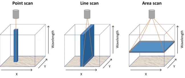
There is a number of approaches for acquiring the hyperspectral images depending on the configuration of pixels in the hyperspectral camera. Wu and Sun (2013) highlighted the most common possibilities. It is point scan, line scan, area scan, which are presented in Figure 5, and single shot scan. For single point scan, each pixel is acquired separately by moving the camera in 𝑋 and 𝑌 direction while acquiring the whole spectra 𝑊. Line scan has an array of pixels of size 𝑁 oriented in direction 𝑦 acquiring the complete spectral information 𝑊. Image is therefore obtained by moving the camera in direction 𝑋. Area scan covers a complete scanned area of 𝑀 × 𝑁, while taking the picture in only one wavelength 𝜆. Therefore, the hyperspectral image is obtained by changing the 𝜆 for the same spatial are of 𝑀 × 𝑁. And finally, single shot scan acquires the complete hypercube 𝑀 × 𝑁 × 𝑊 in one shot.
Figure 5: Types of scanning methods in hyperspectral imaging
Compared to single-point spectroscopy, more information about the sample is acquired and it allows spatial analysis. But a tradeoff of this approach is a larger amount of data that increases demands for computational power (Amigo et al., 2015). A large amount of data can actually pose a problem for subsequent analysis of the hyperspectral image because not all
10
the data in the hyperspectral image are necessary and it can lead to overly complex models and overfitting. It is generally referred to as curse of dimensionality (Camps-Valls and Bruzzone, 2005, Lin and Yan, 2015). Therefore, data reduction or models that can handle the problem are needed.
On the other hand, hyperspectral imaging can have additional advantages compared to single-point spectroscopy, as spatial information can also be used to increase the accuracy of pixel classification. By including spatial information into the algorithm of pixel classification, Fauvel et al. (2013) reached an increase in accuracy of up to 15%, Li and Du (2014) reached an increase of around 10%, or Picon et al. (2010) reached an increase of even 30%, but for example in case of study by Li et al. (2017) the increase was 5% maximum. Wu and Sun (2013) also highlight that compared to single-point spectroscopy, hyperspectral imaging is more suitable for detection of small objects and is more flexible for extraction of spectral information.
2.2 Chemometrics and machine learning
As it was mentioned in the chapter 2.1.1, to interpret NIR spectra there is a need for advanced data analytic methods. Set of these methods applied to data related to chemical properties and composition is generally referred to as Chemometrics. These methods are most
commonly supervised or unsupervised machine learning algorithms combined with data and signal processing.
2.2.1 Data pre-processing
The important first step before acquiring the spectral data from a sensor or a camera is calibration. It is usually done during installation of the device by trained personnel, but because of possible changes of climatic conditions in the laboratory (temperature and humidity change) or technical changes (change in lighting), regular calibration of the device is needed. It is done using dark and white reference (Serranti et al., 2012, Tatzer et al., 2005). Acquired spectrum is adjusted according to the following equation;
𝐼 = 𝐼0− 𝐼𝐵
𝐼𝑊− 𝐼𝐵 Equation 5
In the equation, 𝐼 represents spectra after calibration, 𝐼0 is spectra acquired from the sample, 𝐼𝐵 is spectra of dark reference. It is usually obtained by covering the sensor or camera lens and it accounts for a noise. White reference is spectra 𝐼𝑊 of material with very high diffuse reflectance, usually white ceramic tile or similar material.
Before further use of the data, it needs to be pre-processed to smoothen the spectra and eliminate remaining noise and other negative effects. A number of methods is used in the field of spectroscopy and hyperspectral imaging. Most common ones are Savitzky-Golay filter for smoothening and Standard Normal Variate (SNV) or Multiplicative Scatter Correction
11
(MSC) for the elimination of light scattering effect (Amigo et al., 2015, Cen and He, 2007, Reich, 2005, Wu and Sun, 2013).
2.2.2 Basics of machine learning
Machine learning is using input data to identify and recognize patterns and similarities in data. Learning is done by automatically adjusting parameters of the machine learning model with a goal to minimize error rates of the model. Two general classes of machine learning are supervised and unsupervised learning. Supervised models use response variables, which in case of spectroscopy represent properties of the examined material. The response variables are part of the input data for training and the model searches for relations between
prediction and response variables. In the case of absorbance spectroscopy, prediction variables are given by absorbance of light at various wavelengths. Unsupervised machine learning is distinguished from the supervised one by the absence of response variables. The model uses only prediction variables to recognize patterns and relations among the
prediction variables (Shalev-Shwartz, 2014).
When creating a supervised machine learning model, there are two main stages in the process. First one is the training stage, where parameters of the model are tuned to predict the response variables with the highest accuracy possible. In the second stage, which is validation, the model is tested by inputting new data for the same prediction variables into the tuned model and comparing model’s predictions to reference values. The correctness of prediction is a key measure of model’s performance. It is important to note that the same data mustn’t be used for both training and validation, as the main goal is to see how the trained model behaves for new data. A model that has high accuracy for training data and low accuracy for validation is an overfitted model (Shalev-Shwartz, 2014).
Knowing this, chemometrics in spectroscopy can be simply described as a method that uses spectral information (prediction variables) and known properties of training samples (response variables) to identify properties of tested samples.
2.2.3 Quantitative methods
Quantitative methods are used to quantify some property of the examined material based on the input data. These properties must be numeric, for example temperature, moisture content, or thickness. The most common methods used in spectroscopy are linear methods. These methods look for linear relations between prediction and response variables,
expressing the response variable as a linear combination of prediction variables. The most basic model can be Multivariate Linear Regression (MLR), which uses all
prediction variables and expresses response variable as a linear combination of prediction variables. This approach becomes problematic when there are many prediction variables that don’t have any influence on response variables. In these cases, MLR models tend to overfit and don’t perform well during validation and external validation. To avoid this, pattern recognition techniques are used to eliminate prediction variables with low influence on the response variables. Two most common ones are Principal Component Analysis (PCA) and
12
Partial Least Square (PLS). PCA maps prediction variables into a lower dimensional space of principal components (PC) with a goal of expressing most of the variance in the data with the lowest number of principal components possible. Compared to this, PLS maps both
prediction and response variables into a lower dimension space with the goal to explain the most variance in the response variable with the lowest number of latent variables (LV) possible. In case that variance in response variable is related to maximal variance in the prediction variables (PV), both methods reach approximately the same projection, as shown in Figure 6, where the brightness of points is the response variable.
Figure 6: Mapping by PLS and PCA
Difference between these two methods becomes obvious when the highest variability in the prediction variables does not account for the highest variability in response variables. For examples, if PV1 had a very high inaccuracy of measurement, generating a lot of random variance that has no effect on response variable, results of the mapping would start to differ.
Figure 7: Mapping by PLS and PCA with random noise
Using the mapping into the new subspace, a regression model can be created. Most
commonly used one in the branch on NIR spectroscopy is PLS regression (PLS-R) (Cen and He, 2007, Skvaril et al., 2015, Skvaril et al., 2017b, Wu and Sun, 2013). The model combines mapping into a new subspace of latent variables, which is done by a linear combination of PVs, and regression. Regression is also a linear combination. As LVs are linear combinations of PVs, and RV is linear combinations of LVs, RV can be expressed directly as the linear combination of PVs. This relation is expressed by Equation 6. The regression is done by a set of N + 1 regression coefficients (RC), where N is a number of initial prediction variables and additional coefficient RC0 accounts for bias. Regression coefficients close to zero indicate a
low influence of given PV on the response variable (RV), whereas high positive coefficients account for the increase of response variable and opposite.
13 𝑅𝑉 = 𝑅𝐶0+ ∑ 𝑃𝑉𝑖× 𝑅𝐶𝑖 𝑁 𝑖=1 Equation 6 2.2.4 Qualitative methods
The quantitative methods are used to identify certain qualities of the examined materials that cannot be numerically evaluated. Examples of such qualities can be material type or color. Using these methods, materials can be classified into specified classes representing the qualities.
Many different machine learning algorithms are used in the field of spectroscopy for classification. They can be generally divided into three categories; linear methods, support vector machines (SVM) and artificial neural networks (ANN). They differ in complexity, demand for computational power and accuracy.
Linear methods are probably most widely used in chemometrics (Amigo et al., 2015, Serranti et al., 2012, Tatzer et al., 2005) as they are very simple and efficient while demanding a low amount of computational power. PLS Discriminant Analysis (PLS-DA) and Linear
Discriminant Analysis work on a similar principle as PLS-R, but with a goal to maximize separability of response variables. Also, whereas PLS-DA reduces the number of prediction variables by mapping into lower dimensional subspace, LDA maintains the number of prediction variables and is sensitive to collinearity (one prediction variable being linearly dependent on another). The basic principle of mapping original prediction variables (PVs) to lower dimensional space of latent variables using PLS-DA to maximize the separability of groups is presented in Figure 8.
Figure 8: Basic principle of PLS-DA and maximizing separability
The response variable is represented in these models by discriminants. If the model discriminates 𝐾 classes, then K discriminants are used. If a point belongs to the i-th class, then i-th discriminant has a numeric value of 1 and all the other discriminants have a value of 0 or -1. During prediction, the data point is considered to belong to an i-th class is the i-th discriminant has the highest value of all or if its value is higher than a threshold.
Support vector machines are also widely used algorithms in the field of spectroscopy (Camps-Valls and Bruzzone, 2005, Fauvel et al., 2013, Li et al., 2017, Lin and Yan, 2015, Tarabalka et al., 2010). Compared to the above mentioned methods, SVM searches for decision boundary
14
that separates different classes, as shown in Figure 9. The decision boundaries are defined by support vectors (SV) that are perpendicular to the decision boundary.
Figure 9: Basic principle of the support vector machine
SVM generally reaches higher accuracies than PLS-DA and LDA methods and enables also a non-linear separation of data, but it has higher computational cost and complexity of the model increases exponentially with a number of classes. On the other hand, it is less sensitive to the curse of dimensionality mentioned in chapter 2.1.2.
Lately, use of artificial neural networks have been gaining popularity in the field as suggested by Cen and He (2007), Roggo et al. (2007), Wu and Sun (2013) because they are able to cover complex non-linear dependencies. Advanced architectures like convolutional neural
networks have been applied on hyperspectral images, reaching good results as they are able to cover both spectral and spatial information (Li et al., 2017, Yu et al., 2017). A problem of the approach is that it has high computational cost and requires a large amount of training data. Though, simple ANN architectures proved to perform also very well. In particular, Radial Basis Neural Network (RBNN) showed better results than linear methods (Camps-Valls and Bruzzone, 2005), having comparable results to SVM (Camps-(Camps-Valls and Bruzzone, 2005, Li et al., 2015) while demanding much less computational power then SVM (Li et al., 2015). The method is based on calculating a distance from a classified point to neurons, as shown in Figure 10, and feeding it into Gaussian radial function.
15
2.2.5 Workflow of data handling
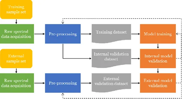
The process of handling follows a general workflow. After the spectral data is acquired, it is pre-processed and used for training (sometimes also referred to as calibration) of a model. Performance of the model is then assessed through validation, which can be internal or external. Internal validation can be used when there is more than one data point available per sample, or when there is very little available data and cross-validation must be used. If
possible, validation using an external sample set should be preferred over internal validation.
Figure 11: General workflow of the chemometric process
Above mentioned k-fold cross validation is a process used when there is very little data for training, so no data can be held out for validation. During k-fold cross-validation, k loops of training are performed, when in each loop, 1/k data points are held out for validation and
(k-1)/k data points is used for training. The dataset for validation is different in every loop, and
after k loops, every data point was used for both validation and training, but never for both at the same time. The final performance of the model is the average of the performance during k loops.
There are also additional steps that can be possibly taken during the data handling process. For example, reducing the data by either by using only certain spectral bands, by spectral or special binning (merging data points) or through PLS or PCA algorithms. For hyperspectral data, results can be also further improved by applying image processing techniques (Amigo et al., 2015).
After the model is validated and its performance is assessed, based on the results, parameters of pre-processing or training can be altered to increase the performance of the model.
Therefore, it can be considered as an iterative process of finding the most suitable model setup.
16
2.3 Applications of NIR spectroscopy
NIR spectroscopy is a very useful method in many fields for a number of reasons. It is a fast, non-destructive, contactless method for material classification and detection of chemical and physical properties.
In pharmaceutic industry (Reich, 2005, Roggo et al., 2007) and in the food industry (Cen and He, 2007, Huang et al., 2014, Wu and Sun, 2013), it is used primarily for quality assessment. It provides an option to quickly and reliably assess chemical composition of samples and identify the presence of unwanted substances or possible chemical changes that are important in these branches. As it all can be done in the real time, it is often applied in production lines. Single-point measurements were often used for continuous homogenous streams, like feeds of liquid or powders, whereas hyperspectral imaging was used for
separation of samples with defects, or when samples on a conveyor belt were distributed with low density and high spread. Deeper penetration of NIR light was also used for quality
control of packaged goods, as samples could be recognized through the packaging layer. Another field where hyperspectral imaging is widely used is aerial and satellite imagery (Benediktsson et al., 2005, Camps-Valls and Bruzzone, 2005, Fauvel et al., 2013, Lin and Yan, 2015, Tarabalka et al., 2010). Using hyperspectral data in the visible to NIR range, it enables the classification of features in the image, like water, grass, forest, roads, buildings, their segmentation, and evaluation of the land cover. The large variability of the
hyperspectral data and a low number of labeled data points (response variable data) is typical for the application. Application of image processing techniques and advanced classification algorithms, mainly SVM, is also common as it can handle previously stated problems well. In the energy and waste field, there has also been a number of applications of NIR
spectroscopy. The most common one is for classification of sorting using hyperspectral imaging for plastics. Amigo et al. (2015) developed a system using hyperspectral imaging at the spectral range 1000-1700 nm, to distinguish 5 types of plastic (ABS, PA, PBT, PP, PS) in form of pure pellets. He used pre-processing by SGF smoothening and 1st derivative and
PLS-DA model, reaching an accuracy of over 94% for all these materials. Ulrici et al. (2013) reached accuracies of over 98% for the distinction of PET and PLA in form of pure
translucent flat tiles, and background made of white ceramic tile. He used the PLS-DA model combined with 2nd derivative and mean pre-processing, analyzing a spectral range of
1000-1700 nm. Serranti et al. (2011) analyzed samples of construction waste containing PP, PE, wood, foam, and aluminum. Samples were placed on a white background, scanned in the spectral range of 1000-1700 nm. He concludes based on PCA analysis that all five materials should be separable, but no model for automatic separation was developed. Even though high accuracies were reached during these studies, it is important to note that they used several simplifications compared to the potential real industrial application. Firstly, in the first two cases highly homogenous samples were used for both training and external validation, which leads to very low variability in the data, making it easier to develop an accurate model. Secondly, in the second and third study, a highly reflective background was used for scanning, compared to the material of a conveyor belt made of dark rubber, again with possible influence on classification accuracy. Closest to the industrial conditions came Zheng
17
et al. (2018) during classification of 6 types of plastic (ABS, PET, PVC, PP, PS, and PE). Spectral data from a range of 1000-2500 nm were pre-processed by SGF 1st derivative and
mean centering and classified using a combination of PCA and Fisher’s discriminant analysis (similar to LDA). The accuracy of classification was 100%, though it is important to note that this was accounted on an object level, not for each pixel.
Apart from plastics, Tatzer et al. (2005) applied hyperspectral imaging in a range of 900-1700 nm to distinguish raw and colored cardboard, newspapers, and white paper. She used a combination of PCA, LDA, and k-nearest neighbor classification applied on relative diffuse reflectance data without pre-processing. Classification accuracy reached over 90% except for colored cardboard, for which it was only 81%.
Single-point NIR is also commonly used in the energy and waste field. Dahl (2018) conducted a deep study of using NIR spectroscopy to determine the amount of fossil origin content in a mixture of artificial RDF. This mixture composed of six types of plastic (LDPE, HDPE, PP, PS, PET, PVC), organic waste, paper, textile and wood, all in a dry form. He then evaluated the amount of plastics in mass percentage, using FT-NIR sensor in the range of 833-2500 nm. After experimenting with various pre-processing methods, his PLS-R model reached R2
value of up to 0.85 for baseline correction (shifting spectrum so that minimum value is zero), though best pre-processing differed significantly depending on model setup.
Skvaril et al. (2015), Winn et al. (2017) used NIR spectroscopy to detect glass on a
homogenous background (made of wood, coconut, rice, or whey) and reached satisfactory results when combining PLS-R model with pre-processing by SGF and SNV. They also concluded that clear glass is harder to detect compared to colored glass. On the other hand, Hedlund (2018) reached very low accuracy of glass detection when using real RDF mixed with glass. He argues that it is due to glass sinking to the bottom of the RDF mixture and therefore not being visible for the NIR sensor.
Skvaril et al. (2017b) also highlight possibilities to apply NIR spectroscopy on the characterization of solid biofuels, particularly reaching good accuracy of prediction for moisture content (R2 = 0.88 for cross-validation) and heating value (R2 = 0.85 for
cross-validation) (Skvaril et al., 2017a). He used spectral data from a range of 1111-2500 nm, PLS-R model and pre-processing by MSC.
Andrés and Bona (2005), Wang et al. (2014) applied NIR spectroscopy for characterization of coal’s properties, reaching good results for moisture, ash, volatile matter, and fixed carbon content. Wang et al. (2014) also observed noticeable improvement in the model’s accuracy when using SVM compared PLS.
18
2.4 Waste and refuse derived fuel
2.4.1 Waste-to-energy combustion plant
Waste-to-energy (W2E) thermal power plants use waste material as fuel to combust it. Heat from combustion is then converted into electric energy through a steam turbine, it can be transferred into a district heating network, or it can be utilized directly as in utility boilers for cement kilns.
Design of boilers in the W2E plants depends on the type of waste that is being combusted. Thorin et al. (2011) with reference to European Commission (2006) documents suggest that most commonly used type of boiler for municipal solid waste (MSW) is reciprocating grate boiler. For pre-treated waste, it is reciprocating or rotary grate boiler.
Combustion of waste in circulating fluidized bed (CFB) boiler is a state of art option that is becoming more and more common. Results from the operation of this type of boiler show that CFB boiler has high combustion efficiency, is more stable even with varying fuel input and has overall lower emissions of pollutants compared to traditional types of boilers (Gulyurtlu et al., 2006, Ravelli et al., 2008).
In case of block 6 (167 MW thermal power) at Mälarenergi’s Västerås powerplant, refuse derived fuel (RDF) is combusted in a circulating fluidized bed boiler. Scheme of the boiler is presented in Figure 12.
Figure 12: Circulating fluidized bed boiler at Västerås (block 6) – scheme created and used with permission from Valmet
19
2.4.2 Preparation of refuse derived fuel
There is a number of issues connected to direct combustion of MSW. It has very low heating value due to high moisture content and a large fraction of incombustible materials. It also contains a fraction of materials that could be separated beforehand and be recycled, therefore decreasing the environmental impact of the MSW combustion.
Thorin et al. (2011) provide an overview of the W2E field and preparation of RDF.
Referencing European Commission (2006) documents, it is highlighted that the main goal of MSW treatment for combustion is to increase its lower heating value and homogenize it. It is generally done by mechanical treatment or by biological treatment. Mechanical treatment consists mainly of sorting and size manipulation. Sorting can be done either manually by workers or automatically. Size of the waste material can be either reduced by milling, shredding or cutting, but also increased by pressing or agglomeration into pellets or
briquettes. Biological treatment is done by digestion and drying. The goal of those processes is to stabilize the biological activity in the waste material, decrease its moisture content and volume.
Setups of RDF preparation differ plant to plant. Various studies also present several
combinations of above-described steps (Bessi et al., 2016, Chang et al., 1997, Gallardo et al., 2014, Guziana et al., 2011). Montejo et al. (2011) compare the composition of input MSW and output RDF. The preparation process in the case of his study consists of two steps of manual sorting, trommel separation, magnetic separation and Foucault separation (for separation of aluminum). The process led to an increase of lower heating value from 8.3 MJ/kg to 16.7 MJ/kg for wet material. Figure 13 shows a comparison of the composition of the waste
material stream before and after processing (with fractions of less than 5 wt.% grouped under category Others).
Figure 13: Comparison of MSW and RDF composition – data retrieved from Montejo et al. (2011)
2.4.3 Emerging methods for composition characterization
Compared to other commonly used fuels, RDF is significantly more heterogeneous and its composition changes depending on the source or even time of the year (Rotter et al., 2011). Because of this, various methods are being developed to characterize the waste and RDF
56.3 13.8 10.7 4.12.6 12.5
MSW
23.7 27.9 24.5 5.8 8.7 9.4RDF
Organic matter Paper and cardboard PlasticsCellulose Textiles Others
20
stream as efficiently as possible. It would enable faster deployment of standards for the alternative fuel and development of markets for RDF and Solid Recovery Fuel (SRF). Schwarzbock et al. (2017) present applicability of a balance method on waste incineration plant for characterization of plastic content in the feed. The method is based on a
combination of sampling and continuous measurements. It determines the plastic content by observing parameters of mass flow, ash content, carbon content, heating value, oxygen consumption, and CO2 production.
Rotter et al. (2011) propose a method based on continuous analysis of flue gases to determine basic characteristics of the input RDF stream as heating value, chlorine content, ash content, and water content. The method combines infrared spectroscopy and ionic chromatography for the flue gases.
Danias and Liodakis (2018), Robinson et al. (2016) reached good results for determination of RDF’s composition using thermogravimetry. The approach is based on slowly heating up samples with constant temperature gradient until 800 °C and observation of sample’s mass decrease depending on the temperature. Combined with data analysis methods and machine learning, they were able to identify individual components like plastics, wood, or paper, but also other properties like water content, ash content, or fixed carbon content.
2.4.4 Common components
As mentioned earlier, the exact composition of RDF and waste varies over time and is also very dependent on place of origin. Particularly for Municipal Solid Waste (MSW),
composition differs from country to country and city to city. Therefore, it is not possible to specify a standard RDF and waste composition. On the other hand, key components are usually common for most of the sources. These component materials that usually account for at least 2% of the total weight, are specified in Table 1.
Table 1: Common components of RDF and MSW
Material Studies that confirm this material present in RDF/MSW
Cardboard (Danias and Liodakis, 2018, Finnveden et al., 2005, Gallardo et al., 2014, Sarc and Lorber, 2013, Schwarzböck et al., 2016)
Food (Chang et al., 1997, Finnveden et al., 2005, Gallardo et al., 2014, Sarc and Lorber, 2013)
Glass (Chang et al., 1997, Gallardo et al., 2014, Sarc and Lorber, 2013) Metals and
ceramics (Chang et al., 1997, Gallardo et al., 2014, Sarc and Lorber, 2013) Newsprint (Danias and Liodakis, 2018, Finnveden et al., 2005, Gallardo et al.,
2014, Haydary, 2016) PE
(LDPE/HDPE) (Danias and Liodakis, 2018, Finnveden et al., 2005, Gallardo et al., 2014, Haydary, 2016, Schwarzböck et al., 2016, Schwarzbock et al., 2017)
21
PET (Danias and Liodakis, 2018, Finnveden et al., 2005, Gallardo et al., 2014, Hiromi Ariyaratne et al., 2012, Schwarzböck et al., 2016, Schwarzbock et al., 2017)
PP (Danias and Liodakis, 2018, Finnveden et al., 2005, Gallardo et al., 2014, Schwarzbock et al., 2017)
PS (Danias and Liodakis, 2018, Finnveden et al., 2005, Gallardo et al., 2014, Haydary, 2016, Schwarzböck et al., 2016, Schwarzbock et al., 2017)
PU (Haydary, 2016, Schwarzbock et al., 2017)
PVC (Danias and Liodakis, 2018, Finnveden et al., 2005, Hiromi Ariyaratne et al., 2012, Schwarzbock et al., 2017)
Textiles (Gallardo et al., 2014, Sarc and Lorber, 2013)
White paper (Chang et al., 1997, Danias and Liodakis, 2018, Gallardo et al., 2014, Haydary, 2016, Hiromi Ariyaratne et al., 2012, Sarc and Lorber, 2013, Schwarzböck et al., 2016)
Wood (Chang et al., 1997, Danias and Liodakis, 2018, Finnveden et al., 2005, Hiromi Ariyaratne et al., 2012, Sarc and Lorber, 2013)
Some of the materials in Table 1 can be present in an amount lower than 2% of total weight. It is mainly some of the individual types of plastic and incombustibles like glass, metals, and ceramics. They are mentioned in the table nevertheless because they have significance in the overall composition. The distinction between individual types of plastics is important for material sorting and content of incombustible materials plays an important role in boiler operation.
2.5 Problems caused by the presence of chlorine
Many studies across the field conclude that chlorine is one of the main problems that is faced while using waste as a fuel (Hunsinger and Andersson, 2014, Lee et al., 2007, Ma et al., 2010, Silva et al., 2014, Sudo et al., 2015, Ma and Rotter, 2008). It is because of chlorine-related high-temperature corrosion damaging heat exchanging surfaces, with severe effect mainly on superheaters, because superheaters are first heat exchangers that come in contact with the hot flue gas after leaving combustion chamber, as it can be seen in Figure 12.
Chlorine has been reported to cause corrosion not only for cheaper low-alloy steel but also for higher quality alloyed steels like chromium steels (Grabke et al., 1995, Viklund, 2011). This leads to unscheduled downtime, increased maintenance costs and decreased efficiency of the plant, as high-temperature corrosion limits the maximal parameters of output steam.
According to Lee et al. (2007), chlorine related corrosion in plants burning RDF or MSW leads up to 20 days/year of unscheduled downtime and accounts for 1/3 of overall maintenance costs.


![Table 2: Order of total chlorine content value for waste fractions [wt.% of dry component]](https://thumb-eu.123doks.com/thumbv2/5dokorg/4947513.136123/37.892.107.781.944.1158/table-order-total-chlorine-content-value-fractions-component.webp)