Subphotospheric dissipation in gamma-ray bursts observed by the Fermi Gamma-ray Space Telescope

Licentiate Thesis in Physics

Subphotospheric dissipation in Fermi

GRBs

Bj¨orn Ahlgren

Particle and Astroparticle Physics, Department of Physics, Royal Institute of Technology, SE-106 91 Stockholm, Sweden

lution of one of the DREAM model’s parameters, L0,52, as a result of time resolved

spectral analysis of this burst. Figure produced by Bj¨orn Ahlgren.

Akademisk avhandling som med tillst˚and av Kungliga Tekniska h¨ogskolan i Stock-holm framl¨agges till o↵entlig granskning f¨or avl¨aggande av teknologie licentiatexa-men fredagen den 10 februari 2017 kl 10:15 i sal FB42, AlbaNova Universitetscent-rum, Roslagstullsbacken 21, Stockholm.

Avhandlingen f¨orsvaras p˚a engelska.

TRITA-FYS 2016:81 ISSN 0280-316X

ISRN KTH/FYS/--16:81--SE

c Bj¨orn Ahlgren, December 2016 Printed by Universitetsservice US-AB

Abstract

Gamma-ray bursts (GRBs) are the brightest events in the Universe, for a short time outshining the rest of the Universe combined, as they explode with isotropic equivalent luminosities up to 1054 _{erg s} 1_{. These events are believed to be}

con-nected to supernovae and to binary compact object mergers, such as binary neutron stars or neutron star – black hole systems. The origin of the so-called prompt emis-sion in GRBs remains an unsolved problem, although some progress is being made. Spectral analysis of prompt emission has traditionally been performed with the Band function, an empirical model with no physical interpretation, and it is just recently that physical models have started to be fitted to data. This thesis presents spectral analysis of GRB data from the Fermi Gamma-ray Space Telescope using a physical model for subphotospheric dissipation. The model is developed using a numerical code and implemented as a table model in XSPEC. Paper I presents

the model and provides a proof-of-concept of fitting GRB data with such a model. Specifically, two GRBs are fitted and compared with the corresponding Band func-tion fits. In paper II, a sample of 37 bursts are fitted with an extended version of the model and improved analysis tools. Overall, about a third of the fitted spectra can be described by the model. From these fits it is concluded that the scenario of subphotospheric dissipation can describe all spectral shapes present in the sam-ple. The key characteristic of the spectra that are not fitted by the model is that they are very luminous. Within the context of the model, this suggests that the assumption of internal shocks as a dissipation mechanism cannot explain the full population of GRBs. Alternatively, additional emission components may required. The thesis concludes that subphotospheric dissipation is viable as a possible origin of GRB prompt emission. Furthermore, it shows the importance of using physically motivated models when analysing GRBs.

Sammanfattning

Gammablixar str˚alar starkare ¨an resten av universum sammanlagt n¨ar de exploderar, och de frig¨or upp till 1054_{erg s} 1_{, om de skulle str˚ala isotropiskt. Detta motsvarar}

ungef¨ar samma energi som finns i hela solen, men frig¨ors typiskt inom loppet av n˚agra sekunder. Dessa h¨andelser tros vara kopplade till supernovor, i fallet med l˚anga gammablixtar, och kolliderande neutronstj¨arnor, eller en neutronstj¨arna som kolliderar med ett svart h˚al, f¨or korta gammablixtar. Man delar upp emissionen fr˚an en gammablixt i tv˚a epoker, den tidiga str˚alningen och eftergl¨oden. Den tidiga str˚alningens ursprung ¨ar fortfarande en obesvarad fr˚aga, trots stora anstr¨angningar f¨or att l¨osa mysteriet om hur den skapas.

Traditionellt sett har spektralanalys av gammablixtspektrum gjorts med den s˚a kallade Band-funktionen, vilket ¨ar en empirisk model f¨or gammablixtspektra, best˚aende av en mjukt bruten potensfunktion. Band-funktionen har ingen fysikalisk tolkning och det ¨ar endast nyligen som fysikaliska modeller har b¨orjat anpassats mot data.

Den h¨ar avhandlingen behandlar den tidiga str˚alningen fr˚an gammablixtar samt f¨ors¨ok att beskriva den med en model f¨or subfotosf¨arisk dissipering. Avhandlingen presenterar spektralanalys med modellen av gammablixtar med data fr˚an Fermi Gamma-ray Space Telescope. Modellen bygger p˚a en numerisk kod som simulerar subfotosf¨arisk dissipering i gammablixtar. Dissiperingsmekanismen som anv¨ands i koden ¨ar baserad p˚a interna shocker. Genom att genomf¨ora ett stort antal simu-leringar kan en s˚a kallad tabell-modell byggas upp, vilken kan anpassas till data i spektralanalysprogrammetXSPEC.

Artikel I beskriver hur tabell-modellen konstrueras, samt ¨ar en konceptvalidering f¨or tabell-modeller inom spektralanalys f¨or gammablixtar och f¨or att anpassa data med en fysikalisk modell. I det h¨ar pappret anpassas modellen till data fr˚an tv˚a gammablixtar och resultaten j¨amf¨ors med motsvarande anpassningar med Band-funktionen. Slutsatsen ¨ar, f¨orutom att demonstrera metoden, att modellen kan beskriva flera typer av spektrum, som inom ramen f¨or Band-modellen ofta beskriver med extra spektralkomponenter.

I artikel II utvecklas modellen f¨or subfotosf¨arisk dissipering vidare, parameter-rymden f¨or modellen utvidgas och analysverktygen f¨orb¨attras. Dessutom intro-duceras adiabatisk kylning i modellen, en mer ing˚aende analys av os¨akerheter i modellen och i anpassningarna genomf¨ors. Tv˚a scenarion med olika magnetisering

i gammablixtarnas utfl¨ode unders¨oks; ingen magnetisering samt m˚attlig magne-tisering. Fr˚an dessa scenarion skapas tv˚a tabell-modeller vilka anpassas mot 37 gammablixtar. Resultatet blir att sammanlagt ungef¨ar en tredjedel av alla anal-yserade spektrum kan beskrivas av n˚agon av tabell-modellerna, samt att dessa modeller inte kan s¨arskiljas av datan. Vidare dras slutsatsen att modellerna f¨or subfotosf¨arisk dissipering kan ˚aterskapa alla de spektralformer som finns represen-terade bland de 37 gammablixtar som analyseras h¨ar, och att de spektrum som inte kunnat beskrivas med n˚agon av modellerna ¨ar v¨aldigt ljusstarka. Dessutom sammanfattas anledningen till att dessa ljusstarka spektra inte kan beskrivas av n˚agon av modellerna, med att de underliggande antaganden som interna shocker som dissiperingsmekanism f¨or med sig, inte till˚ater reproducering av tillr¨ackligt stor normalisering. Slutligen visar artikeln vikten av att beskriva dessa spektrum med fysikaliska modeller.

Acknowledgments

First, I would like to thank my supervisor, Josefin Larsson, for her support and patience, and for being so generous with her time. I would also like to thank my co-supervisor, Felix Ryde, for helping out with all manner of things, for promoting my work, and for introducing me to people when I least expect it.

I would also like to take this opportunity to thank the people I work with, particularly; Edvin, with whom I shared an office until his strategic escape to Switzerland, for all the times I could interrupt him in his work to discuss something. Vlasta for the countless (technically not true, but who keeps track) times she has joined me for a short break and her infectious enthusiasm. And Damien, for always stopping by to ask me if I want to join for lunch, despite the statistically verified bleak prospects of that enterprise.

Lastly, I would like to thank my wonderful girlfriend and sambo, Nabila, for always being there and being the best imaginable support. And my amazing friends, particularly Martin, Emil, Axel and Johanna, and many others, you know who you are.

So far the journey has been both interesting and entertaining, and I expect that it will get even better!

Contents

1.3 Emission phases and light curves . . . 3

1.4 Relativistic outflows in GRBs . . . 3

1.4.1 Spectral features . . . 5

2 Theory and modelling 7 2.1 Relativistic outflows and frames of reference . . . 7

2.2 The fireball model . . . 9

2.3 Dissipation mechanisms . . . 11

3 Observations and data analysis 13 3.1 The Fermi Gamma-ray Space Telescope: detectors, data products and performance . . . 13 3.1.1 GBM . . . 13 3.1.2 LAT . . . 14 3.1.3 Data reduction . . . 15 3.2 Analysis . . . 18 ix

4 The DREAM model 21 4.1 Observational justification and physical scenario . . . 21 4.2 Numerical code . . . 22 4.3 The Table Model . . . 26

Summary of the attached papers 29

Author’s contribution to the attached papers 31

List of figures 33

Outline

This thesis is structured such that it starts with a general introduction, followed by four chapters introducing gamma-ray bursts (GRBs) and some of the key concepts of the work.

Chapter 1 is devoted to giving an overview of GRBs, including their progenitors and emission properties. In chapter 2 I go through some of the basic theoretical concepts that lay the foundation to the work in the thesis, such as relativistic Doppler shift and frames of reference. Chapter 3 describes GRB observations, as well as the instrument with which the data I examine has been gathered. Finally, in chapter 4, I introduce the physical model, and what has been done to make it possible to fit it to data. This model has been one of the main goals of this thesis to produce and to test. I also describe the numerical code from which the model is built.

The bulk of the work is then presented in the form of two articles, appended at the back of the thesis, of which the first article is published and the second is a draft of an article which is soon to be submitted.

Introduction

Gamma-ray Bursts (GRBs) are rare, cosmological events, isotropically distributed on the gamma-ray sky. Despite being rare on a cosmological level we are currently observing, on average, about one burst every day. This is due to the extreme nature of GRBs. A GRB is the release of a tremendous amount of energy in gamma-rays, the isotropic equivalence of up to a solar mass of energy, in a time span of between a fraction of a second and a couple of minutes. The extreme luminosities, L ⇠ 1050 54_{erg/s, for isotropic equivalent energies, make these events not only visible}

at cosmological distances, but also the most distant objects in the Universe that we are able to detect. Fig. 1 shows the distribution of observed GRBs as a function of redshift. The average redshift of detected GRBs is_{⇠ 2, which corresponds to a} distance of about 5_{⇥ 10}10_{light years, respectively.}

GRBs were first observed in 1967, by the VELA satellites as brief flashes of gamma-rays of extraterrestrial origin. It was not until several years later, 1973, that the findings were published in [1]. At this point it was completely unknown what these events were, as was their extragalactic origin. It was not until the 1990’s that it was concluded that the observed GRBs were indeed not from our own galaxy. One of the keys to this conclusion is their angular distribution. With the Burst and Transient Source Experiment (BATSE), which was mounted on the Compton Gamma Ray Observatory (CGRO), it was possible to determine GRB positions precise enough to infer that they are isotropically distributed across the sky [2].

With the launch of the Beppo-SAX satellite in 1997 and its subsequent mea-surement of fading X-ray signals in some GRBs it was discovered that GRBs in addition to their prompt gamma-ray emission also have afterglows at longer wave-lengths [3]. It was the discovery of the afterglow and the fact that it lasts long enough for follow up observations in optical and radio wavelengths that allowed for sufficiently precise localisation to identify host galaxies and their corresponding redshift [4]. This settled the question of their extragalactic origin.

0

2

4

6

8

10

Redshift

0.0

0.1

0.2

0.3

0.4

N

or

ma

li

se

d

fr

eq

u

en

cy

Chapter 1

Gamma-ray bursts

Here I briefly present our current understanding of GRBs and outline some of the models used to describe the di↵erent phases of GRBs as well as some of the characteristic spectral features of the radiation. For a more complete overview of GRBs, see e.g. [5, 6].

1.1

Introduction

With the launch of BATSE the number of detected bursts increased rapidly and by analysing burst durations, two classes of GRBs, long and short, were found [7]. The simplest way to show this is to plot a histogram of burst durations in logarithmic scale where two populations are visible to the naked eye, with a divisor at ⇠ 2 seconds, which has been set as the delimiter between the two populations. Since it might be ambiguous when a burst has ended, the T90 is used instead, which is

defined as the time when 90 percent of the radiation has been observed. There have been claims of more than two populations [8, 9], but there is no conclusive evidence and the statistical significance of introducing additional populations is negligible [10].

The long bursts have been found to associate with high redshifts, typically 1-2, whereas the short bursts are typically found at lower redshifts, though it is generally harder to measure the redshift for short bursts [11]. Furthermore, we observe more long bursts than short bursts and the short bursts also have an isotropic equivalent luminosity which is typically a few orders of magnitude lower than that of long bursts [12, 13, 14].

1.2

Progenitors

Observations indicate that long GRBs are associated with core collapse supernovae. The first joint detection of a GRB with a supernova came in 1998 when a supernova

was discovered in the vicinity of GRB 980425 [15]. This gave strong support for the connection between supernovae and GRBs. Since then there have been many joint observations of GRBs and supernovae, including spectroscopic analysis and measured redshifts, which have confirmed that the events are related [16]. Further analysis of long GRBs have revealed that they are mainly found in galaxies with high star forming rates [17], which is also consistent with them being related to the death of massive stars.

Short GRBs is a more elusive matter, but theoretical models suggested, and in-direct observations later confirmed, that short GRBs are likely the result of compact object mergers (neutron star-neutron star or black hole-neutron star) [18]. This has not yet been confirmed by direct detections, but the compact object merger sce-nario remains the most plausible model. However, the closest to a direct detection so far is likely the kilonova association of GRB 130603B [19]. Since long GRBs make out the majority of observed GRBs, between 70-90 percent [20], along with their relatively long duration which facilitates follow up observations, these have been studied in greater detail than short bursts. However, there have still been afterglows observed for short GRBs, which reveal that they are found in a plethora of galaxies, not necessarily ones with high star formation rate [21, 22]. Additionally, they can be found outside of their host galaxies, which is consistent with the binary merger scenario.

Regardless of the progenitor it is believed that the main source of the GRB en-ergy comes from accretion of matter onto a compact object, releasing gravitational energy. This process is one of the most efficient means of releasing energy, in the Universe. Whether the progenitor is a massive star or compact object mergers we expect a black hole to form, along with an accretion disk. It is a fraction of the energy released by the gravitational collapse of this disk that yields the electromag-netic radiation we observe in the prompt emission. Furthermore, this is essentially why we would not expect GRBs as a result of a binary black hole merger, as this is thought to be a clean system with little matter to accrete. However, there are models predicting GRBs from such systems [23]. Additionally, if the progenitor is a massive star undergoing core collapse we expect the majority of the energy to be released in the form of thermal neutrinos. In the event of compact object mergers we would expect a significant fraction of the energy to be converted into gravitational waves.

There is another model scenario, in which, rather than form a black hole, a rapidly rotating proto-neutron star is created. For a rotational period of _{⇠ 1 ms} and surface magnetic fields on the order of 1015 _{G, this is known as a magnetar}

[24, 25]. In this scenario, the energy released in the collapse, or merger, is con-verted into magnetic fields, which yield a Poynting flux dominated outflow. This magnetic energy then propels the jet out from the magnetar [26], leading to the prompt emission. One observational justification for this model is a plateau like featured in the X-ray band observed by the SWIFT satellite in some GRBs [27, 28]. This behaviour can be explained for magnetically dominated outflow by letting the plateau be the result of residual rotational or magnetic energy which may continue

1.4. Relativistic outflows in GRBs 3

to inject energy into the outflow at these later stages [29].

1.3

Emission phases and light curves

As already mentioned, GRB emission is divided into two parts; prompt emission and afterglow. Despite its short duration, the bulk of the electromagnetic radiation emitted in a GRB lies in the prompt emission.

There are several features of prompt GRB emission, but the single most striking characteristic is likely that GRB lightcurve seem to be unique. There appears to be no pattern in how the lightcurve will vary, nor for how long the emission will continue or how many peaks it will have. Fig 1.1 contains examples of 12 light curves, that clearly display this apparent erratic behaviour. A recurring feature is that the prompt emission is sometimes foregone by a short precursor. This is seen in the lightcurve as a small, brief spike, usually a few seconds up to minutes prior to the bulk of the prompt emission.

Burst durations vary widely and span more than six decades in time, from 0.01 seconds for the shortest bursts up to several hours for the bursts with the longest durations, e.g. GRB 111209A, which has a duration of more than seven hours [30]. Burst duration is not the only temporal attribute to vary between bursts; the variability time is another useful concept in GRB physics and is derived from the width of the peaks in the lightcurve. Variability has been observed down to a level of milliseconds in some long bursts [31]. The observed variability sets powerful constraints on theoretical models.

Regardless of the underlying emission mechanisms of prompt emission and of progenitor we would expect the emerging jet to produce shocks as it collides in the surrounding medium. These shocks produce radiation at lower energies and longer time scales than the prompt emission. When the afterglow was first discovered by Beppo-SAX it was in terms of fading X-emission from GRB 970228, found eight hours after the detection of the prompt emission, which later also led to the first optical afterglow [3]. The X-ray emission was observed to fade in a power law fashion over a few days, a predicted behaviour for X-ray afterglows [32]. Since then, the expected infra-red and radio counterparts have been found as well [33].

This thesis’ main concern is a specific model for the production of the GRB prompt emission.

1.4

Relativistic outflows in GRBs

Due to the already mentioned fast variability of GRBs we can conclude that the size of the emitting region must be small. The fastest variabilities observed at the ⇠millisecond level correspond to an emitting region of ⇠ 107_{cm, approximately the}

same size as a Schwarzschild radius of a 30 solar mass black hole, in order for time delay from di↵erent regions of the source not to smear the signal. Given the small emission regions and and the high isotropic equivalent luminosity of typical bursts,

Figure 1.1. Example of light curves. The figure is made by Daniel Perley using data from the public BATSE archive, http://gammaray.msfc.nasa.gov/batse/grb/catalog/.

1.4. Relativistic outflows in GRBs 5

the radiation would be optically thick due to pair production of photon-photon interactions, leading to suppression of the high-energy emission. For the radiation to escape we infer relativistic outflows with high Lorentz factor, typically inferred to be in excess of 100, meaning that the outflow is highly relativistic and beamed, see e.g. [34].

There are several additional arguments for why GRBs should emit in relativistic outflows, including observed jet-breaks in GRB afterglows [35]. In many bursts, a steep decay in the afterglow can be observed about a day after the burst, with the emission going as a power law t p_{, with typically p}

⇠ 2 [36, 37]. This e↵ect is caused by two things; firstly, the edge of the jet becoming visible as it slows down. This is a result of relativistic beaming (relativistic beaming is covered in section 2), where an observer located along the jet axis perceives the radiation to be isotropic form the source. As the Lorentz factor of the outflow decreases, more of the jet becomes visible to the observer due to the opening angle of the photon beaming increasing, until photons from the entire width of the jet reaches the observer. When the Lorentz factor decreases further, the increased spreading of the photons from any given part of the jet is no longer compensated by more of the jet becoming visible, and there is a sudden drop in observed flux. Secondly, as the jet slows down it starts for spread laterally, further decreasing the emission, which has been shown to occur at a similar time as the first e↵ect [35, 37]. Finally, GRBs are not the only phenomena to have beamed emission, jets have been directly observed for Active Galactic Nuclei (AGN) and is no uncommon occurrence in the Universe.

Another feature of jetted emission is that this relaxes the energy requirements of bursts. As noted in the introduction, the isotropic equivalent energies released are huge, and challenging to model. When calculating the isotropic equivalent energy it is assumed that the energy released from the GRB is emitted equally in every direction, and hence the the total energy required would decrease by up to a few orders of magnitude if the bursts instead emitted radiation in jets [36].

1.4.1

Spectral features

GRB prompt spectra are usually described by the so called Band function [38], which is a smoothly broken power law, defined as

N (E) = ( E↵_exp⇣ E E0 ⌘ , if E_{ (↵} )E0 [(↵ ) E0](↵ )E exp ( ↵), if E > (↵ )E0 , (1.1)

with N (E), being the photon number spectrum, ↵ the slope of the low energy power law, the slope of the high energy power law, and E0 the break energy.

Addition-ally, there is a normalisation parameter. The Band model is an empirical function and does not correspond to any physical scenario, even if some e↵ort has been made to reconcile it with e.g. synchrotron radiation. Although the model lacks a physical interpretation, it does provide several interesting relations between its parameters and physical quantities, such as the Amati relation, which shows a correlation be-tween the observed peak energy, Ep=(2+↵)E_↵ 0, and the isotropic equivalent energy,

Eiso [39]. The Band model has had remarkable success at consistently describing

Chapter 2

Theory and modelling

In this chapter I briefly present some of the key concepts behind GRB physics. More extensive descriptions of these concepts can be found in the reviews by [40, 41, 42, 6].

2.1

Relativistic outflows and frames of reference

Working with velocities close to that of the speed of light, c, one encounters the theory of relativity and particular frames of reference become important. In this section I state the Lorentz transformation, present the Doppler shift formula for relativistic outflows and discuss the most important frames needed. Starting from the theory of relativity, the Lorentz transformation between two frames of reference, K and K0_{, can be written as}

x0= (x vt) (2.1) y0= y (2.2) z0= z (2.3) t0= ✓ t cx ◆ , (2.4)

where primed coordinates pertain to the comoving frame, K0. This notation will be maintained throughout the thesis. It is assumed that K0 moves with a uniform speed v along the x coordinate and that their origins coincide at t = 0. Furthermore,

= v/c and is the Lorentz factor, defined as

=p 1 1 2.

This leads to the concept of length contraction, such that a rigid rod of length L0 = x01 x00, when travelling in the comoving frame K0, the length as measured

in the rest frame K becomes L = x1 x0 = L0/ , using Eq. 2.1-2.4. Hence the

rod appears to be shorter by a factor of 1/ when measured in a frame where it is perceived to be moving. Naturally this e↵ect is symmetrical between the two frames and hence an observer in the frame K0 would likewise consider the same rod, now being at rest in frame K to be similarly contracted by the factor 1/ . However, there is no paradox involved in this e↵ect and the di↵erence in perceived length is an e↵ect of what is considered to be simultaneous events in the two frames. When a stick is measured in a frame, both ends of the stick are measured simultaneously in that frame, but not according to an observer in another frame. Using similar logic it is easy to show that time dilation obeys T = T0_{, where T and T}0 _{is the}

duration of a process as measured in the frames K and K0_{, respectively. Thus, a}

process in the comoving frame appears to last longer when measured in the rest frame.

When discussing these concepts in an astrophysical setting, there are a few stan-dard frames of reference, pertaining to di↵erent situations. The lab frame refers to the frame where the jet is moving at relativistic speeds, , and where the progenitor is non-moving, i.e. the stellar rest frame for our purposes. Additionally, there is the observer frame, which is the same as the lab frame, down to the cosmological redshift factor, associated with cosmological distances due to the expansion of the Universe. This induces a shift of energies from the cosmological lab frame by a factor 1/(1 + z) in the observer frame, i.e. Elab_{/(1 + z) = E}obs_.

Finally, I will consider photons from relativistic sources as observed in the lab frame. Although time dilation will make processes in K0 _{appear longer than in}

K there is an additional e↵ect to take in to account when considering photons from sources propagating with relativistic velocities. If the source is assumed to propagate at an angle ✓ and with a relativistic velocity , relative to the observer situated in the lab frame, a photon emitted at time t0 and one emitted at t1 is

observed with a time di↵erence of tobs_{= t}0 _{(1 cos ✓) = t}0_{/D, where t}obs

denotes the observed time di↵erence and where I have introduced the Doppler shift formula,

D = ₍₁ 1_{cos ✓)}. (2.5) Similarly, the observed frequency of a photon emitted from a relativistic source is ⌫ =D⌫0_{. Additionally, the comoving temperature transforms as T =DT}0_.

It is illustrative to consider this Doppler factor for di↵erent angles, ✓. For ✓ = ⇡, i.e. for a receding source, D _{⇠ 1/2 , whereas for an approaching source,} with ✓ = 0, a series expansion of ( ) yields D_{⇠ 2 .}

Additionally, when considering an isotropically emitting source, travelling at rel-ativistic speeds towards an observer, the radiation is beamed towards the observer. Consider a photon which is emitted at a comoving angle of ✓0 _{=±⇡/2, with respect}

to the direction of motion of the source. This angle is given by sin ✓ =_{±1/ in the} lab frame, and for 1, this becomes ✓ ⇠ ±1/ . This is known as relativistic beaming, and is, apart from being a fundamental feature of relativistic sources, important when considering e.g. jet geometries.

2.2. The fireball model 9

2.2

The fireball model

Here I present the schematics of the most popular GRB model; the fireball model [43, 44, 45, 46]. For recent reviews of the fireball model, see the references given at the beginning of this chapter. I outline the derivations of the scaling laws for the temperature of the plasma, as well as the Lorentz factor of the bulk outflow, and define the saturation radius and the photospheric radius.

Beginning from the arguments presented in section 1.4, a huge energy, typically in excess of 1052 _{erg, is released in the collapse of a massive star, or through the}

merging of two compact objects. This energy is assumed to be released in a few milliseconds inside a volume approximately the size of a Schwartzchild radius. In the centre of the explosion, a compact object, either a black hole or a magnetar, is formed, onto which the surrounding material can accrete and possibly supply more energy to the GRB. However, the nature of this process is not well understood. The majority of the energy is converted into neutrinos and gravitational waves, which can escape the GRB unhindered. A small fraction, a few per mille to a few percent of the energy, forms an opaque fireball in the form of a plasma of e±_,

photons and baryons. Due to the high opacity the fireball is in thermal equilibrium at this stage. Additionally, there are scenarios where the outflow may also carry magnetic fields with comparable energy content to that of the rest of the fireball. The dynamics of the outflow, and thus the scaling laws presented below, depend on the magnetisation. Below I assume the fireball to be photon-dominated, a so-called ”hot fireball”, with low magnetisation. Conversely, an outflow dominated by magnetisation is known as a ”cold fireball”, and will not be covered here.

The fireball experiences a sufficiently high radiation pressure from the photons to counteract the gravitational pressure, meaning that it starts expanding. The threshold is given by the Eddington luminosity, LE = 4⇡GM mpc/ T, with G

being the gravitational constant and T the Thomson cross section, which is the

luminosity where radiation pressure balances gravitational pressure. For a one solar mass object this becomes LE(1M ) ⇠ 1038 erg s 1, orders of magnitude

below observed GRB luminosities. As the plasma expands, it accelerates until some threshold velocity, after which it continues to propagate with a coasting Lorentz factor = ⌘, where ⌘ _{⌘ L/ ˙}M c2 _{is the dimensionless entropy of the outflow. I}

motivate the value of this entropy below, when I discuss the saturation radius. The temperature of the plasma at the base of the outflow is given by the energy density of the emitting region through Stefan-Boltzmann’s law as

aT04= L/(4⇡r02c), (2.6)

where a is the radiation constant, giving us a temperature of

T0= ✓ L 4⇡r2 0ca ◆1/4 . (2.7)

Note that the outflow is considered to be photon dominated and that photons outnumber leptons and baryons by several orders of magnitude.

To obtain the scaling laws of the fireball, conservation of energy and entropy is used, and the evolution of the temperature in the fireball is followed. Assuming that the energy is released and contained in a shell of width r ⇠ r0, giving it a

comoving volume of V0_{= 4⇡ r}0_r2_{= 4⇡r}

0 (r)r2, the observed total energy of the

shell in the lab frame is

Eobs

/ (r)V0(r)T0(r)4_{= (r)}2_r2_r

0T0(r)4, (2.8)

which is constant due to conservation of energy. As previously, primed quanti-ties belong to the comoving frame. Considering entropy from the relation dS = (dU + pdV )/T , the entropy of the outflow in the comoving frame is found as S0 _{= V}0_(u0_{+ p}0_)/T0_{, where u and p are the internal energy density and internal}

pressure, respectively. Note that the chemical potential has been set to zero since I consider a photon dominated outflow. Furthermore, in a radiation dominated outflow it holds that p0_{= u}0_{/3/ T}04_{, as given by Eq. 2.6. Hence,}

S0= V0u01 +

1 3

T0_(r) / r0 (r)r

2_T0_(r)3_{= const, (2.9)}

where I have neglected the rest mass as well as the initial kinetic energy of the baryons, meaning that the entropy pertains to the photons. Combining Eq. 2.8 and 2.9 results in an observed temperature T (r) = (r)T0(r) = const. This is an expected result, meaning that as the comoving temperature decreases, the Lorentz factor of the outflow will increase. Hence, as the outflow expands, internal energy of the radiation will be converted into kinetic energy of the outflow. It is obvious that this expansion cannot go on forever and that there is a saturation radius, rs,

at which the Lorentz factor coasts, such that rs ⌘ ⌘r0, again with the previously

defined ⌘_{⌘ L/ ˙}M c2_{. This means that the acceleration cannot continue, since the}

Lorentz factor per particle cannot increase beyond the initial value of internal energy per particle of the plasma. Alternatively, it can be understood as the particles start out with individual Lorentz factors _{⇠ ⌘, with an isotropic velocity distribution,} and that at rs, the velocities are contained within an angle rs/r0. Note also that

at rs, most of the energy is in the form of kinetic energy of the baryons.

Although the outflow ceases to accelerate it continues to expand and hence the temperature will decrease and Eq. 2.9 yields that T0_{(r)/ r} 2/3_{. Summarising the}

scaling laws in the two di↵erent regimes discussed so far yields

(r) = ⇢ r r0 r < rs ⌘ r > rs, (2.10) T (r) = ⇢ T0 r < rs T0(r/rs) 2/3 r > rs, (2.11) V0(r)/ ⇢ r3 _{r < r} s r2 r > rs, (2.12)

2.3. Dissipation mechanisms 11

In the above reasoning I have assumed that the plasma is optically thick as long as r < rs and that the energy is released momentarily in a shell of width r0. For

bursts of duration longer than r0/c the emission can be considered to consist of

many sub-shells, each of width r0 and follow the above reasoning. There are also

several other approaches to derive the standard fireball scenario, but the method outlined above highlights some important aspects which are important for the work in this thesis and the discussions to follow.

Finally, the spectrum is released at the photosphere, which is the surface of last scattering, given by ⌧ = 1, with ⌧ being the optical depth. For a relativistic outflow the optical depth at a given radius is given by ⌧ = (L T)/(8⇡r 3mpc3), where T

is the Thomson cross section and mpis the proton mass [47]. Solving this equation

for r and setting ⌧ = 1 gives the photospheric radius as rph= (L T)/(8⇡ 3mpc3).

If the radiation leaving the photosphere has been unaltered from the scenario described above, the observed prompt emission would be a Planck function, which is not the case. There are several ways to obtain non-thermal spectra, of which I will discuss a few in the next section.

2.3

Dissipation mechanisms

There are several possible mechanisms to dissipate energy in a GRB outflow. Gen-erally, dissipation means that energy is transferred to the electrons in the outflow by tapping energy from either the bulk kinetic energy of the baryons, or the magnetic fields present. Magnetic energy can be accessed through magnetic reconnection, where magnetic field lines of di↵erent magnetic domains meet and change their pattern of connectivity [25]. Kinetic energy of the bulk motion can be dissipated by shocks, where shells of di↵erent velocities collide and transfer energy by Fermi acceleration [48]. There are di↵erent types of shocks suggested for dissipation in GRBs; external shocks [49, 46], hadronic collision shocks [50] or internal shocks [51]. In this section I will discuss internal shocks and sketch the derivation of the central properties of a basic internal shock scenario, since this particular dissipation mechanism is assumed in the numerical code that has been employed in Paper I and II.

The internal shock scenario is derived from the fireball model. As stated in the previous section, continuous emission can be considered to consist of independent sub-shells, each typically of width_{⇠ r}0. It is assumed that there are fluctuations in

the central engine activity on the time scale of t = r0/c, which is the observed

vari-ability time. The fluctuations in the outflow leads to the shells obtaining slightly di↵erent densities which results in di↵erent coasting Lorentz factors, usually as-sumed to be of order _{⇠ ⌘, where ⌘ is the typical value of the coasting Lorentz} factor for the shells. This leads to a velocity spread of v _{⇠ c/2⌘}2 _{between two}

shells. Hence, faster shells will catch up to slower shells ahead of them and create shocks that propagate into the colliding shells. A forward shock will propagate into the slower shell and a reverse shock will propagate into the faster shell. This converts kinetic energy of the bulk flow motion into internal energy of the outflow.

Given the shell width, r = r0, and velocity of the shells, they will start to

collide at a radius rd= 2r0 2. The merge time for the two shells in the comoving

frame is given by t0merge = r0/c = r0/c. In the lab frame this becomes tmerge=

r0/c = tobs, with tobs being the observed variability time of the burst. Hence

internal shocks give observed variability times on the same scale as the central engine activity. Note that it is possible for these shocks to take place below or above the photosphere.

It should be noted that internal shocks have a very limited efficiency. It is clear that the two colliding shells can dissipate no more energy than the di↵erential kinetic energy between them. Consider two shells, with m1, m2 and 1, 2 as

the respective shell’s mass and Lorentz factor. It was showed by [52], assuming

1, 2 1, that the resulting Lorentz factor of the merged shell becomes

f = [(m1 1+ m2 2)/(m1/ 1+ m2/ 2)]1/2. (2.13)

This leads to an efficiency of

e = 1 (m1+ m2) f m1 1+ m2 2

,

which, together with Eq. (2.13) shows that, as expected, similar masses, m1⇠ m2

and a large di↵erence in Lorentz factors, 1 2, is required for highest efficiency.

Using typical values of GRBs, and taking into consideration that a first shock with high efficiency leads to lower efficiency for subsequent collisions due to the high merged Lorentz factor, f, it has been shown that the typical total efficiency

expected is 1 10% [53, 52, 54, 55, 56].

The internal shock scenario’s strength is the model’s simplicity, as well as its ability to reproduce the fastest observed variabilities. Its main weakness is the low efficiency, requiring large luminosities to produce the observed fluxes. Furthermore, it lacks predictive power since it does not make any predictions about the details of the emission; how long it will be, spectral features or amount of dissipated energy.

Chapter 3

Observations and data

analysis

In this chapter I describe the observational data used in this thesis, I give an overview of the data reduction, the experiment used to gather the data, and the software and principles used to analyse the data.

3.1

The Fermi Gamma-ray Space Telescope:

detectors, data products and performance

The Fermi satellite was launched on June 11th, 2008 and orbits Earth in a low-earth orbit, with an orbital period of 90 minutes. The satellite carries two experiments; the Gamma-ray Burst Monitor (GBM) [57], and the Large Area Telescope (LAT), [58], two wide field instruments for observing emission in the gamma-ray part of the spectrum.

3.1.1

GBM

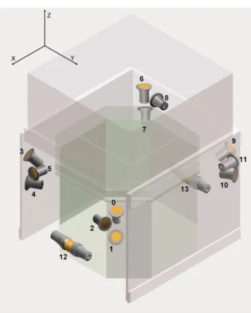
The GBM covers an energy range of 8 – 40 000 keV, and is composed of 12 sodium iodide (NaI) scintillation detectors, operating in the energy range 8 keV – 1000 keV , and two bismuth germenate (BGO) scintillation detectors, operating in the energy range 200 keV – 40 000 keV. The NaI detectors are comprised of a crystal disk, 12.7 cm in diameter and 1.27 cm in thickness attached to a photomultiplier tube (PMT). Fig. 3.1 shows a photograph of an NaI detector flight unit. The GBM has a detection rate of⇠ 240 bursts/year [10].

The BGOs, similarly, consist of crystal cylinders, 12.7 cm in diameter and con-nected to PMTs that convert detected photons to electrical signals. Fig. 3.2 shows a photograph of a BGO detector flight unit. Since these units have an energy de-tection range that overlaps with that of the NaI detectors, and the LAT, which

Figure 3.1. NaI(Tl)-detector flight unit. The figure is from Fig. 3 in [57].

is described further down in the text, they allow for cross calibration between the instruments and detectors.

The Nai detectors are arranged such that the relative counting rates can be used to infer the position of observed GRBs. The two BGOs are positioned on each side of the space craft in order to ensure that at least one of them detects any given burst occurring above the horizon. In Fig. 3.3 the positions and orientations of the di↵erent detectors on GBM are shown.

There are three e↵ects that can cause problems at high photon-rates; detector dead time, pile-up in the electronics, and data loss due to the limited data transfer speed from the GBM to the spacecraft for download to Earth. These e↵ects are not limiting factors for most bursts, with only one exception to the third e↵ect. In GRB 130427A [59], there was ensuing data loss due to limits in the transfer speed of 1.5 MB s 1_{, as well as pile-up and dead times.}

3.1.2

LAT

The LAT is a telescope based on pair-conversion, and detects photons in the energy range below 20 MeV to above 300 GeV [58], spanning 4 orders of magnitude of high-energy gamma-rays. It has a detection rate of_{⇠ 10 15 bursts/year [60]. The LAT} allows for timing and direction measurements along with its energy measurements of incident photons. It may also redirect towards bright bursts located by the GBM. It consists of a calorimeter, precision tracker and anti-coincidence detector for rejecting charged particle background events

3.1. The Fermi Gamma-ray Space Telescope: detectors, data products and performance15

Figure 3.2. BGO detector unit, from Fig. 5 in [58].

A pair-conversion telescope functions by letting photons of energy twice the rest mass energy of the electron, E 2mec2, interact with the high Z-material

of the detector and create electron-positron pairs. Since energy and momentum is conserved and can be retrieved through detection by the electron and positron, the original photons energy and momentum, and hence its direction, can be inferred. The energies of the charged particles are measured by the calorimeter and their directions are obtained by having their path’s registered by the precision tracker.

The calorimeter consists of 16 calorimeter modules, each situated below a tracker module so that both energy and momentum can be retrieved. The calorimeter modules consists of thallium activated caesium iodide (CsI(Tl)) crystals, and each calorimeter module is made up of 96 crystals. When a charged particle enters the calorimeter it will create a shower of secondary particles which will give rise to energy deposition events in the crystals. Each such event registers the amount of energy deposited and the physical position of the event. Together with leakage corrections, this allows for precise reconstruction of the shower and thus the original particle and finally the photon.

3.1.3

Data reduction

The resulting data files, from the LAT and the GBM, are event files for each detector, containing information about each individual photon detected. Using one type of such files, the tte-files, from a given detector, a light curve can be created using e.g. the Fermi tool, gtbin. Additionally, spectral files can be created with the same tool, making PHA (Pulse Height Analyser) files, for spectral analysis. In order to remove the background from the data when analysing transients, the background is modelled by a low-order polynomial, fitted to the data by using the

Figure 3.3. Schematics of detector positions and orientation on the GBM. The NaI detectors are indexed 0-11 and the BGOs are denoted by 12 and 13 in the figure. The gray box is the LAT. The figure is taken from Fig. 4 in [57].

3.1. The Fermi Gamma-ray Space Telescope: detectors, data products and performance17 20 0 20 40 60

Time(s)

Co

u

nt

s

Figure 3.4. Example of a fit of a low-order polynomial to the background of a burst. The burst in this example is 091127. The green lines indicate the chosen burst interval, the red is the best-fitting polynomial, and the region outlined by the blue line represents the region excluded from the fitting.

data before and after the event as constraints. In Fig. 3.4 I present an example of what such a fit may look like. Finally there is the response files, which contain information about the instrument response, i.e. the information relating incoming photons to detected counts in the detector. Hence, the result of the data reduction is the three data files containing information about the burst, the background and the instrument response, for each detector. When choosing detectors to use for the analysis, the detectors with the lowest angle towards the source are used, with an upper cut of 60 towards the source also applied. Generally, no more than three NaI detectors are used, and always one BGO detector [10].

Apart from the pure GBM and LAT data there is a third category of data products available for GRB analysis from Fermi. The LAT-Low Energy (LLE) data are a type of LAT data designed for the use with bright transients to bridge the energy range of the LAT and GBM [61]. The LAT-LLE data allows fitting in the energy range 30–1000 MeV.

3.2

Analysis

In this thesis, spectra are fitted using the standard software packageXSPEC[62]. The

software uses the PHA, background, and response files mentioned in the previous section.

The procedure for fitting a model to this data is to use forward folding [63]. With this technique, a model is required before a spectrum can be produced, meaning that it is impossible to describe spectral shapes without first having a model. The model must be convolved with the detector response, yielding the model’s count prediction, which may be compared with the detected counts. The model parameters are then varied in order to find the best fit of the model counts to the detected counts, i.e. the minimal di↵erence between the two. The result is then given as the best-fitting parameters for the model, which produce the best agreement with the data. What is registered in the detector is not the spectrum, but photon counts in given instrument channels. The spectrum is then given from the integral equation

C(I) = Z 1

0

f (E)R(I, E)dE, (3.1)

where I is the instrument channels, C(I) is the detected counts as a function of channel, R(I, E), the detector response as a function of energy and channel, and f (E) is the actual spectrum from the source. If it were possible to invert Eq. (3.1), the true spectrum could be obtained without fitting a model. However, as it turns out, this is usually not the case. Due to the non-linearity of the processes involved, R(I, E) is singular, and inversions yield non-unique, unstable solutions, see e.g. [64, 65, 66].

The use of forward folding introduces some very important caveats to keep in mind: the results obtained are biased by the initial hypothesis since the fitted model is pre-determined. This means that some features of the data may be completely invisible for certain choices of model. Secondly, the data can be equally well fitted by two di↵erent models.

The fitting described above is performed using maximum likelihood statistics, using the idea that the best-fitting parameter values maximise the probability of the observed data given the model. The likelihood is defined as the total probability of observing the data given the model and parameter values. However, for simplicity, it is usually two times the negative log likelihood which is used.

The likelihood will look di↵erent depending on the nature of the data. The primary concern for GRB spectral analysis is that the data is Poisson distributed. The fact that the count rate is rather low makes any Gaussian approximations poor, and Poisson statistics must be employed. Additionally, there is a non-negligible background present, which is usually modelled in the way described above. This yields an uncertainty in the background, assumed to be Gaussian. For this purpose there is the pgstat statistics, which is Poisson distributed data with a Gaussian distributed background [62]. This is the likelihood statistic used in all GRB spectral analysis in this thesis.

3.2. Analysis 19

Parameter errors calculated in XSPEC are obtained by fixing the parameter of

interest and fitting for the other parameters. The value of the fixed parameter is then changed and the model is then again fitted for all other parameters. This process is repeated until the desired change in fit statistic value is obtained. To find the parameter values at the end of the confidence intervals, XSPEC employs

a bracketing algorithm and then an iterative cubic interpolation. The errors can also be computed, with less accuracy, using the Fisher information, which can be obtained by inverting the covariance matrix.

However, neither of these two approaches this captures the true errors for most models, and a more robust and accurate approach is to perform Monte Carlo (MC) simulations. A large number of spectra are simulated from the best-fitting spec-trum, and the model is then re-fit to each spectrum. In this way the distribution of the model parameters is acquired for the given spectrum, from which the errors can be calculated. XSPEChas built-in functionality to support for this general method,

using the command fakeit, to simulate fake spectra from a given spectrum. The downside with this approach is that it is more computationally expensive.

Chapter 4

The DREAM model

In this Chapter I describe the model for subphotospheric dissipation used in this work. I outline the functionality of the numerical code used to model it and go through the physical scenario in the framework of the code. Finally, I discuss the creation of DREAM (Dissipation with Radiative Emission as A table Model), the resulting table model and some of its features.

4.1

Observational justification and physical

scenario

The idea of a photospheric origin of GRB prompt emission began as early as 1986, with Goodman [43] and Paczynski [44]. However, the notion of photspheric emission was later largely disfavoured by observations, which showed that GRB spectra were far from thermal, mainly through the use of the previously described Band function, see Chapter 1. However, a few bursts were detected with spectra that could be described by a Planck function, [67, 68]. A black body (BB) yields a steep function, with a hard low energy slope, ↵ = 1, in terms of the Band function parameters. It has been shown that synchrotron radiation cannot reproduce a spectrum with a low energy slope harder than ↵ = 2/3, in the slow-cooling regime, and ↵ = 3/2 in the fast-cooling regime. GRBs are likely in the fast cooling regime, since the cooling time sets the variability time scale, and also since a long cooling time would make the burst radiate too inefficiently. Observationally, there are many bursts which are inconsistent with these limits on ↵ [69, 70], thus limiting synchrotron as the source of prompt emission. Conversely, it has been shown that there are multiple mechanisms for making photpsheric emission broader than a Planck function, e.g. geometric e↵ects [71, 72]. Additionally, there are bursts that are described by a BB and an additional component [73, 74, 75, 76]. Hence, the observed bursts that are consistent with simple BB emission dictates that photospheric emission is required as an explanation for at least some bursts, and the fact that it is possible to obtain

photospheric emission that is non-thermal makes a photospheric origin of prompt emission possible for additional bursts.

Apart from geometric broadening, it has been showed that dissipation of kinetic energy in the outflow near the photosphere can significantly alter the spectrum such that a non-thermal shape is recovered from the photosphere [51, 77, 78, 79]. It is this particular scenario that this thesis is concerned with.

4.2

Numerical code

I have used a numerical code by [80], to simulate our physical scenario. For more details see also [81, 82, 83]. In this section primed quantities denote comoving frame, and non-primed quantities are defined in the lab frame.

I use the code to simulate subphotospheric dissipation in an internal shock scenario. The code can in principle handle di↵erent dissipation mechanisms, such as magnetic reconnection [25, 84], or hadronic collision shocks [50]. The main feature of the code that pertains specifically to internal shocks is the relation between the nozzle radius, r0, and the dissipation radius, rd, as presented below and in chapter

2.

The code is a radiative transfer code which solves the kinetic equations of en-ergy transportation. All calculations are performed in the comoving frame and assumes both homogeneous and isotropic distributions of particles and photons in this frame. The computations are carried out in time steps of constant size, with an injection of relativistic electrons in each step, at a constant rate and in a Maxwellian distribution. At each time step, the kinetic equations for the Compton and inverse Compton scattering, cyclo-synchrotron emission, synchrotron self-absorption and pair creation and annihilation are solved numerically, using Cranck-Nickolson inte-gration. In each time step, the energy loss times as well as the annihilation times are calculated for the electrons and positions, and also for the photons. For pho-tons, electrons or positrons for which the energy loss time or annihilation times are found to be shorter than the fixed time step, it is assumed that all energy is lost in a single time step, and these are treated separately. The size of these time steps is set manually and the required step size is dependent on the input parameters. Furthermore, it should be noted that the code sometimes di↵ers by a factor of 2 from the theory presented in Chapter 2, e.g. in the expression of the dissipation radius, since the code removes these factors for simplification. The code outputs a photon energy grid which spans 13 decades of energies, between 10 14 _{and 0.1}

erg, containing the spectrum at rd, as well as the electron and positron spectra, in

energies spanning 6 orders of magnitude, from⇠ 8 · 10 7 _{to 1 erg.}

The following input parameters are used: the luminosity in terms of 1052 _erg

s 1_{, L}

0,52, the optical depth at the site of dissipation, ⌧ , the fraction of dissipated

bulk kinetic energy, "d, the fraction of dissipated energy that goes into the electrons

and magnetic fields, "e and "b, respectively, and the coasting bulk Lorentz factor

of the outflow, . Additionally, there is a parameter "pl, which sets the fraction of

4.2. Numerical code 23

electrons assume a Maxwellian distribution. In the presentation below we let "pl=

0, which does not make any qualitative di↵erence, but simplifies the discussion. It is assumed, in agreement with the internal shock scenario, that shells of width r_{⇠ r}0 are ejected at some nozzle radius r0, due to central engine activity, and

that two shells will start to merge at the dissipation radius, rd, defined through its

optical depth as

rd= L0,52 T

4⇡⌧ c3 3_m p

= 2r0. (4.1)

A time scale t, being the observed variability time of the burst and the time scale over which two shells merge, is defined as t = rd/ 2c. The merger time in

the comoving frame is thus t0dyn = t, which is here referred to as the comoving

dynamical time, and sets the duration of the dissipation in the comoving frame. Hence, the dissipation takes place between rd! 2rd, i.e. between ⌧ ! ⌧/2, which

also corresponds to a distance r0_{, one shell width in the comoving frame. Thus,}

the comoving volume of heated electrons as a function of time will be given by V0 _{= 4⇡r}2

dct0 = 4⇡r2d r0t/tdyn, with t0 being the comoving time. The key radii,

together with the model parameters, are presented in Fig. 4.1. Note that the figure is not to scale.

The shells contain Nshell = L0,52 t/ mpc2 electrons, initially in thermal

equi-librium with the photons. With the internal energy density of the electrons being u0

e = "eu0int = "e"dL0,52/4⇡r2dc 2 and the internal energy of the photons being

u0 _{= aT (r}

d)04, it is useful to define the fraction A = u /ue . Additionally, since

the main source of photons is the thermal seed photons, the ratio of power emit-ted by the electrons in synchrotron and inverse Compton scattering is given by S = Psync/PIC = u0B/u0, with u0B = "bu0int being the comoving energy density of

the magnetic fields.

The comoving normalised temperature of the photons is defined as ✓ = kBT0/mec2.

The photons are initially thermally distributed at this temperature. The heated electrons are injected as a Maxwellian distribution and similarly have a normalised temperature ✓e , defined by the characteristic Lorentz factor of the distribution,

such that ✓e = 0char/2, where the characteristic Lorentz factor of the electrons

in the shell comoving frame is 0

char = 2"e"d(mp/me) [83]. Using this, we can

show that the electrons are expected to lose all their kinetic energy in the co-moving frame during one dynamical time. Electrons of a Lorentz factor 0char lose

their energy by Compton scattering and synchrotron emission over a typical time scale of tloss= E/(dE/dt) = char0 mec2/(4/3)c T char02 u0(1 + S). Thus, they cool

down to ⇠ 1 on the time tloss = tloss char0 . I then obtain the following ratio of

the cooling time and the dynamical time, tloss/tdyn ⇡ 1/((4/3)A(1 + S) char0 ⌧ ) =

(3/4) 2/32 /30⌧ (0.44 + 0.48"B, 0.5"d 1). This yields that for "b⇡ 0.3, "d⇡ 0.1 and ⌧ _{ 1, the electron will cool during the dynamical time as long as  2 · 10}4_{. As}

long as the electrons cool efficiently in the photon field, the spectrum can be sig-nificantly altered by heating of the electrons. The spectrum firstly change in that photons are up-scattered to higher energies, modifying the high-energy part of the

Γ

r

Optically thin region

2rd r0 Nozzle ! radius End of ! dissipation

Figure 4.1. Jet schematics in the framework of the model simulated by the numer-ical code. The model parameters are presented at the di↵erent radii at which they are defined. A luminosity, L0,52, is emitted from the compact object at a nozzle

radius, r0, and travels outwards in a jet. Initially, the radiation pressure accelerates

the outflow such that the Lorentz factor of the outflow increases linearly with radius. At the saturation radius, the Lorentz factor reaches its coasting value, ⌘. At a larger radius, rd, given by the optical depth at the site, ⌧ , dissipation occurs,

con-verting a fraction "dL0,52of the kinetic energy into internal energy of the outflow, of

which a fraction "eand "bgoes into the electrons and magnetic fields, respectively.

An approximation of the model is that the dissipation does not alter the coasting Lorentz factor of the jet. The dissipation continues for one dynamical time, until the radius has doubled, at 2rd. In the current version of the code the spectrum

is instantaneously released at this point. In principle, however, the jet constituents continue to interact until the photosphere is reached, and it is only an approximation of the code that the spectrum is released after the dissipation has finished. Note that the figure is not to scale.

4.2. Numerical code 25

10

₁₀

₁₀

₁₀

₁₀

₁₀

₁₀

Energy (keV)

10

10

10

10

10

10

EF

(k

eV

s

m

)

Figure 4.2. Example of output spectra from the numerical code. The black line represents the spectrum given by [L0,52= 0.1, ⌧ = 1, "d= 0.05, "b= 0.1, = 350],

the red line by [L0,52= 10, ⌧ = 10, "d= 0.1, "b= 10 6, = 100], the blue line by

[L0,52= 10, ⌧ = 20, "d= 0.2, "b= 10 6, = 350], and the magenta line is given

by [L0,52= 0.1, ⌧ = 20, L0,52= 0.1, "d= 0.2, "b= 0.1, = 200]. The small peaks

located at 104 ₁₀5 _{keV are the peaks from pair annihilation.}

spectrum. The low energy part of the spectrum can be modified by synchrotron radiation, which directly may insert photons at low energies, around and below the BB peak. However, even without synchrotron radiation, the low energy part of the spectrum is modified as the BB is destroyed by inverse Compton scattering, which, depending on parameters, can significantly alter the low energy slope and peak po-sition of the spectrum. In Fig. 4.2 we show a few examples of di↵erent characteristic output spectra from the code. In the appended articles I give an overview of the di↵erent impacts on the spectral shape the di↵erent parameters have.

The code does not include adiabatic cooling, in the sense that the photons are instantaneously released after the dissipation. This is a valid approximation if the dissipation ends at ⌧ _{⇠ 1. However, if the dissipation ends below the photosphere,} the photons will continue to interact with the plasma, continuously loosing energy to the bulk motion of the outflow. The loss of energy to the bulk expansion will lead to a constant shift in energy of the entire spectrum. [85] introduces the adiabatic cooling factor, a = 2⌧ 2/3_{, and shows that this factor yields the net e↵ect of pure}

However, the shape of the spectrum will also change, since the photons will be increasingly thermalised by each scattering and the change of energy per scattering will be dependent on the initial photon energy. This cannot be retroactively com-pensated for when considering the emerging spectrum, and must be treated in the code. A detailed discussion of this can be found in paper II.

Another important approximation is that the code does not include any geo-metric e↵ects, since it is 0-dimensional. The main e↵ect of this is that it does not include any hydrodynamics or jet structure, which is a simplification.

4.3

The Table Model

In this section I outline how the code was used to create a model forXSPECwhich

could be fitted to data, and also motivate the specific choice of model parameters. The discussion is brief since these topics are covered in some detail in both paper I and II. The table model was named DREAM (Dissipation with Radiative Emission as A table Model).

Table models are routinely used in X-ray astronomy, e.g. in the analysis of active galactic nuclei (see models by [86, 87]). This thesis introduces the first implementation of a table model for GRB analysis.

I run the numerical code described above for a large number of input parameters. The goal is to test whether subphotospheric dissipation is a viable origin for prompt emission, and the parameters were chosen with this in mind. Obviously, ⌧ > 1 is required. Little change is expected in the spectral shape above some cut o↵ value of the optical depth, and tests showed that ⌧ ⇠ 35 provided an reasonable cut o↵ for our parameter space. The luminosity was chosen to lie in the range 0.1 300L0,52,

so that I simulate bursts in the energy range 1051 3· 1054 _{erg s} 1_{, which covers}

most of the expected GRB luminosities. However, because of "d, these are not the

observed luminosities, which instead are similar to "dL0,52. The Lorentz factor was

chosen to lie in the range 50 500, in the first implementation of the model (Paper I). However, the choice of minimum Lorentz factor was changed between the two articles, since 100 was found to be a sufficiently low limit, rather than 50. "d is

set to be less than 0.5, since too large a value of this parameter would change the physical scenario, because it would significantly lower the kinetic energy of the jet after dissipation. Due to computational reasons, and to minimise degeneracies in the model, "e and "bwere set to constant values, thus leaving four free parameters

of the model.

The simulations span a grid in the parameter space, which, due to technical reasons, must be rectangular. Having four free parameters is enough for the curse of dimensionality to matter, and thus each parameter is not allowed more than 4-9 grid points. The table models used in papers I and II use 500 and 1350 grid points, respectively. The curse of dimensionality, together with the fact that a single run of the code usually takes 1-4 days to complete, sets the limitations on how large and finely spaced parameter grid that can realistically be spanned. Additionally, it is not immediately clear what step size is required for the simulation to converge, hence

4.3. The Table Model 27

a simulation must often be run more than once to ensure proper convergence. For this purpose I have used several super computers to run these simulations, Ferlin and Povel at PDC Center for High Performance Computing at the KTH Royal Institute of Technology, as well as Triolith at the National Supercomputer Centre (NSC) at Link¨oping University.

List of appended Papers

Paper I

Ahlgren et al. (2015), Confronting GRB prompt

emission with a model for subphotospheric

dissipation

In this paper we fit Fermi GRB data with a photospheric emission model which includes dissipation of the jet kinetic energy below the photosphere. We create DREAM (Dissipation with Radiative Emission as A table Model ), a table model forXSPEC, and fit it to GRB 090618 and GRB 100724B, and compare the fits to the

corresponding Band function fits. We conclude that our model can fit both single and double peaked spectra.

Published in Monthly Notices of the Royal Astronomical Society: Let-ters 2015 454 (1): L31-L35 doi: 10.1093/mnrasl/slv114.

Paper II (Draft)

Ahlgren et al. (2017), Subphotospheric dissipation

in GRBs: fits to Fermi data constrain the

dissipation scenario and reveal correlations

In this paper we consider a model for subphotospheric dissipation which produces non-thermal spectra from the photosphere. Building on the work of [88], we consider two di↵erent magnetisation scenarios; no and moderate magnetisation, and create two table models which we fit to 37 bursts using time-resolved analysis. We show that the models can describe about a third of the fitted spectra and that the main reason for a non-successful fit is a lacking normalisation of our model. We conclude that all spectral shapes present in our sample can be fitted and that it is the internal shock paradigm which is the reason for the insufficient normalisation.

Author Contribution

Paper I

I performed all the work in this paper, except creating the code that turns sim-ulation output into a table model, which was created by Tanja Nymark. The manuscript was written by me, with comments from the co-authors. Additionally, all the figures are created by me.

Paper II

All the work was performed by me, except for:

• creating the original Monte Carlo code for error calculations, described in section 4.2 and 4.3, which was created by Erik Ahlberg. However, I made modifications to and developed it.

• The idea of introducing the cooling factor, a, which was suggested by Christof-fer Lundman.

The manuscript was written by me, with comments from the co-authors. Addition-ally, all the figures are created by me.

All work has been performed with the guidance of my supervisor, Josefin Lars-son, and co-supervisor, Felix Ryde.

List of Figures

1 Redshift distribution of detected GRBs with a measured redshift. . xiv

1.1 Example of light curves. The figure is made by Daniel Perley using data from the public BATSE archive,

http://gammaray.msfc.nasa.gov/batse/grb/catalog/. . . 4

3.1 NaI(Tl)-detector flight unit. The figure is from Fig. 3 in [57]. . . . 14

3.2 BGO detector unit, from Fig. 5 in [58]. . . 15

3.3 Schematics of detector positions and orientation on the GBM. The NaI detectors are indexed 0-11 and the BGOs are denoted by 12 and 13 in the figure. The gray box is the LAT. The figure is taken from Fig. 4 in [57]. . . 16

3.4 Example of a fit of a low-order polynomial to the background of a burst. The burst in this example is 091127. The green lines indicate the chosen burst interval, the red is the best-fitting polynomial, and the region outlined by the blue line represents the region excluded from the fitting. . . 17

4.1 Jet schematics in the framework of the model simulated by the nu-merical code. The model parameters are presented at the di↵erent radii at which they are defined. A luminosity, L0,52, is emitted from

the compact object at a nozzle radius, r0, and travels outwards in

a jet. Initially, the radiation pressure accelerates the outflow such that the Lorentz factor of the outflow increases linearly with radius. At the saturation radius, the Lorentz factor reaches its coasting value, ⌘. At a larger radius, rd, given by the optical depth at the

site, ⌧ , dissipation occurs, converting a fraction "dL0,52 of the kinetic

energy into internal energy of the outflow, of which a fraction "e and

"b goes into the electrons and magnetic fields, respectively. An

ap-proximation of the model is that the dissipation does not alter the coasting Lorentz factor of the jet. The dissipation continues for one dynamical time, until the radius has doubled, at 2rd. In the current

version of the code the spectrum is instantaneously released at this point. In principle, however, the jet constituents continue to inter-act until the photosphere is reached, and it is only an approximation of the code that the spectrum is released after the dissipation has finished. Note that the figure is not to scale. . . 24 4.2 Example of output spectra from the numerical code. The black line

represents the spectrum given by [L0,52 = 0.1, ⌧ = 1, "d = 0.05,

"b = 0.1, = 350], the red line by [L0,52 = 10, ⌧ = 10, "d = 0.1,

"b= 10 6, = 100], the blue line by [L0,52 = 10, ⌧ = 20, "d= 0.2,

"b= 10 6, = 350], and the magenta line is given by [L0,52= 0.1,

⌧ = 20, L0,52 = 0.1, "d= 0.2, "b = 0.1, = 200]. The small peaks