Effects of inelastic dark matter in the early Universe

Master thesis

E↵ects of inelastic dark matter

in the early Universe

Daniel Aho

Particle and Astroparticle Physics, Department of Physics, School of Engineering Sciences

KTH Royal Institute of Technology, SE-106 91 Stockholm, Sweden Stockholm, Sweden 2020

Akademisk uppsats f¨or avl¨aggande av Civilingenj¨orsexamen inom utbildningspro-grammet Teknisk Fysik.

Scientific thesis for the degree Master of Science in Engineering Physics. TRITA-SCI-GRU 2019:403

c Daniel Aho, April 2020

Abstract

When we study the Universe, and compare the amount of luminous baryonic matter with observable gravitational e↵ects, we obtain incomprehensible results. It seems as a large portion of the total gravitating mass is missing, and one compelling hypothesis is that the missing part is some kind of unseen gravitational matter, which we call dark matter. Over the years, a great deal of evidence have built up and the dark matter hypothesis is now widely accepted. One promising explanation is that the dark matter are elementary particles, and a lot of e↵ort has been invested in the search for particle physics models that contain dark matter candidates. One of the main motivations is that we know that the standard model of particle physics is incomplete. It is very appealing to search for a new particle physics model that can explain abnormalities in the standard model, while explaining dark matter at the same time.

In this thesis we study an inelastic dark matter model in the early Universe. Through the means of statistical mechanics, the Boltzmann equation describing the freeze out mechanism is derived. The equation is then solved to find the dark matter abundance that would be present in the Universe today. In addition, we study what kind of parameter choices that result in the correct abundance according to recent experiments. It turns out, however, that the particular model of choice leads to some unexpected problems compared to other self-interacting models. We take a closer look at these problems and discuss how they might be resolved. Nevertheless, with some simplifications and bold assumptions, we find that the obtained results are consistent with similar self-interacting dark matter models. Lastly, we highlight the fact that a non-relativistic e↵ect, called Sommerfeld enhancement, might need to be taken into account in order to fully describe freeze out for non-relativistic self-interacting dark matter.

key words: dark matter, self-interactions, inelastic dark matter, freeze out, dark sectors.

N¨ar vi studerar Universum, och j¨amf¨or m¨angden synlig baryonisk massa med dess gravitationella e↵ekter, finner vi obegripliga resultat. Obervationer pekar mot att en stor m¨angd av den gravitationella massan saknas. En ¨overtyganden hypotes ¨ar att den saknade massan ¨ar n˚agon osynlig typ av massa, som vi kallar m¨ork mate-ria. ¨Over tid har en m¨angd bevis byggts upp och m¨ork materia-hypotesen ¨ar nu vitt accepterad. En lovande f¨orklaring ¨ar att den m¨orka materian best˚ar av ele-mentarpartiklar, och stora anstr¨angningar g¨ors f¨or att finna en partikelfysikmodell som inneh˚aller m¨ork materia-kandidater. En av de fr¨amsta motivationerna till det-ta ¨ar att vi vet att den nuvarande sdet-tandardmodellen i partikelfysik ¨ar fel. Det ¨ar v¨aldigt lockande att s¨oka efter en partikelfysikmodell som kan f¨orklara avvikelserna i standardmodellen, och samtidigt f¨orklara vad m¨ork materia ¨ar.

I det h¨ar arbetet studerar vi en inelastisk m¨ork materia-modell i det tidiga Universum. Med statistisk mekanik s˚a h¨arleds Boltzmannekvationen som beskriver hur m¨ork materia fryser ut. Vi l¨oser denna ekvationen f¨or att ber¨akna den abundans som skulle finnas kvar i Universium ¨an idag. Vi studerar ¨aven vilka parameterval som ger oss en abundans som st¨ammer ¨overens med data fr˚an observationer. Det visar sig dock att den s¨arskilda modellen i denna uppsats leder till ov¨antade problem j¨amf¨ort med andra sj¨alvinteragerande modeller. Vi tittar n¨armare p˚a dessa problem och diskuterar hur dessa eventuellt kan l¨osas. Icke desto mindre finner vi, med f¨orenklingar och dj¨arva antagningar, att resultaten ¨ar f¨orenliga med resultaten fr˚an liknande modeller. Till sist s˚a belyser vi det faktum att en icke-relativistisk e↵ekt, kallad Sommerfeld enhancement, kan beh¨ovas tas med i beaktning f¨or att till fullo beskriva hur icke-relativistisk sj¨alvinteragerande m¨ork materia fryser ut.

Nyckelord: m¨ork materia, sj¨alvinteraktioner, inelastisk m¨ork materia, m¨orka sektorer.

Preface

This thesis is the result of my work in the Particle and Astroparticle Physics group at the Department of Physics at KTH Royal Institute of Technology. The thesis is for the degree Master of Science in Engineering Physics, and it treats a particular model of dark matter (DM) and its e↵ects in the early Universe.

Outline of thesis

In Chapter 1, a brief introduction to DM is given. The supporting evidence for the DM hypothesis is discussed and the current understanding of how DM behaves in the Universe is presented. We also look at the currently accepted model of particle physics and we will explore in which way this model can be expanded to include DM in a natural way. Lastly, we will take a brief look at some current and upcoming experiments developed to detect DM. Chapter 2 is about thermal systems at cosmological scales, where an introduction to the framework needed to treat DM in the early Universe will be given. The chapter is then concluded with an illuminating simple freeze out example. In Chapter 3, an inelastic DM model is introduced and motivated. The DM abundance is calculated with numerical methods. In Chapter 4, various problems that arise with the inelastic model are discussed, and we try to pinpoint how these can be resolved. We also discuss a few improvements that can be made for the calculations carried out in Chapter 3. The final Chapter 5 will summarize and conclude this thesis.

Natural units

In theoretical physics and cosmology, it is inconvenient to work in the international system of units (SI) and instead we choose a system where

~ = c = kB = 1. (1)

In the above, ~ is the reduced Planck constant, c the speed of light, and kB is

the Boltzmann constant. This simplifies the notation tremendously and makes the underlying physics more apparent. One single unit is needed to parametrize the rest

Derivation SI Natural units Length _{1 eV}~c 1.97_{· 10} 7_{m 1 eV} 1 Mass 1 eV_c2 1.78· 10 36kg 1 eV Time _{1 eV}~ 6.58_{· 10} 16_{s 1 eV} 1 Temperature 1 eV_k B 1.16· 10 4_{K 1 eV}

Table 1: Conversion table for natural units.

and the most common choice is electronvolt eV. From the conversion Tab. 1, we see that it also makes dimensional analysis easier. In order to check the dimensions of an expression, one simply counts the powers of eV and look in the table to see if the dimensions agree. One more simplification is worth doing when dealing with high-energy physics. In the early Universe temperatures were so high that quantities of the order eV results in rather large numbers to deal with. Therefore, unless stated otherwise, everything in this thesis will be expression in powers of GeV.

Preface vii

Acknowledgements

First of all, I would like to thank my supervisors Dr. Mattias Blennow and Dr. Stefan Clementz, for the opportunity to do my Master thesis in the Particle and Astropar-ticle Physics group. I feel very grateful for their guidance, support, and patience, and I wish them both all the best in the future. I would also like to thank my friends from KTH, for all the good times we shared during these past five years. I will remember this time for the rest of my life. Lastly, I would like to give a special thanks to my girlfriend Malin and to my family, for always believing in me and supporting my choices.

Contents

1.1.1 Galaxy clusters . . . 1

1.1.2 Rotation curves . . . 2

1.1.3 Cosmic microwave background . . . 3

1.1.4 Gravitational Lensing . . . 4

1.2 Dark matter halos . . . 6

1.2.1 Simulations and DM halo structure . . . 6

1.2.2 Small scale structure problems . . . 7

1.3 Particle dark matter . . . 8

1.3.1 The Standard model . . . 8

1.3.2 Dark sectors . . . 9

1.4 Searches for DM . . . 11

1.4.1 Direct detection experiments . . . 11

1.4.2 Indirect detection experiments . . . 12

2 Dark matter in the early Universe 15 2.1 Cosmology . . . 15

2.1.1 Expansion . . . 16

2.1.2 Experimental results . . . 17

2.2 Statistical Mechanics . . . 18

2.2.1 Phase-space and density functions . . . 18

2.2.2 The Boltzmann equation . . . 18

2.3 Freeze out . . . 22

2.3.1 A simple model . . . 22 ix

2.3.2 Cross sections . . . 25

3 Inelastic dark matter 29 3.1 Motivation . . . 29

3.1.1 The small scale structure problems with self-interacting DM 29 3.1.2 Inelastic DM as a possible solution . . . 31

3.2 The inelastic framework . . . 32

3.3 Dark photons and kinetic mixing . . . 33

3.4 Freeze out in the inelastic model . . . 35

3.4.1 Results . . . 38

3.4.2 A few words about the results . . . 39

4 Discussion 43 4.1 Temperature in the dark sector vs the SM sector . . . 43

4.2 Problem with symmetries and amplitudes . . . 45

4.2.1 External gauge bosons in QED . . . 45

4.2.2 QED with a massive gauge boson . . . 47

4.2.3 Majorana mass terms . . . 50

4.3 Sommerfeld enhancement . . . 51

4.4 Possible improvements . . . 53

5 Summary and conclusions 55

Chapter 1

Introduction

To this day, physicists have discovered two very successful fundamental theories for describing the behaviour of Nature, namely the theory of general relativity (GR) and the standard model of particle physics (SM). Thus far, GR, which provides us with a macroscopic unified description of gravity as a geometric property of space-time, has passed every experimental test. To briefly mention two recent examples, we have the direct detection of gravitational waves, done by the LIGO and Virgo collaborations [1], and the first picture of the shadow of a supermassive black hole, obtained by the EHT Collaboration [2]. On the other hand, we know that the SM, which describes the fundamental properties of Nature’s building blocks, i.e., the elementary particles, is wrong. While being able to provide us with some of the best agreements between theory and experiments [3], the SM fails to explain other fundamental properties found for some elementary particles, such as neutrino oscil-lations between the flavour eigenstates [4, 5]. In addition, while several experiments hints that a large portion of the mass in the Universe seems to be non-luminous, the SM gives no clues about what this dark matter (DM) is made of.

1.1

History and supporting evidence

Currently there are many independent sources of evidence at hand that favour DM. The pile of evidence have been building up for the last century, and a few eminent examples will be presented in this section.

1.1.1

Galaxy clusters

The first hints of DM were obtained by Fritz Zwicky in 1933 [6]. By observing the dispersion of velocities in the Coma galaxy cluster, Zwicky found that there were di↵erences in the velocities of at least 1500 to 2000 km/s. If one assumes that

the cluster is in a stationary equilibrium, the virial theorem states that the time average over the total kinetic energy T and potential energy U are related as

hT i = 1₂hUi. (1.1)

The non-relativistic kinetic energy of a galaxy in a cluster is given as T = mv2/2, where m is the mass of the galaxy and v is the velocity with respect to the center of mass of the cluster. Furthermore, the potential energy between two galaxies within the cluster is U = Gmimj/rij, where G is Newton’s constant, mi and mj are the

masses of the two galaxies, and rij is the distance between them. Substituting this

into Eq. (1.1) and summing over all galaxies yields * X i miv2i + = * X i X j<i Gmimj rij + , (1.2)

where the subscripts labels the galaxies. The left side of this equation can be ap-proximated as the total mass M of the cluster multiplied by the mass and time averaged velocity squared v2_{. In addition, by assuming that the galaxies are}

uni-formly distributed over a spherical region, the right hand side can be approximated as GM2_{/R, where R is the radius of the Coma cluster. With these estimations in}

mind, Zwicky derived the relation

M v2 _{= G}M 2

R (1.3)

and from his observations he was able to estimate the parameters. Zwicky found that the mass deduced from the virial theorem exceeded the observed luminous matter by a factor of at least 400. Furthermore, he made the bold claim that if this missing matter is some kind of new invisible matter, then the amount of this invisible matter would be present in a much greater amount than luminous matter, something we believe today to be true. Back then, Zwicky’s work was thought of as controversial and the general opinion was that we simply lacked understanding about the astrophysical systems in question.

1.1.2

Rotation curves

The first really strong indication of DM came from measurements of galaxy rotation curves [7], i.e., the measurements of the rotational velocity v(r) of objects inside a galaxy as a function of the distance to the center r. The idea is very simple and goes as follows. Since the velocities in question are non-relativistic, we can equate the centrifugal force to the force predicted by Newton’s law of gravitation, we find

m(v(r))2 r = G

mM (r)

1.1. History and supporting evidence 3 where G is Newton’s gravitational constant, m is the mass of the object we want study, and M (r) is the total mass enclosed by a sphere of radius r. We can solve for v(r) to obtain

v(r) = r

GM (r)

r , (1.5)

which then tells us that the mass distribution of the galaxy completely determines the rotation curve.

Observations dictate that most of the luminous mass of spiral galaxies is concen-trated in a central bulge of radius r_⇤, so outside this bulge M (r) is approximately constant. Substituting this into Eq. (1.5), we expect to find that v(r) _{⇠ 1/}pr when r > r_⇤. However, in the early 1970s conflicting observational results started to appear, resulting in several important articles [8, 9]. In 1980, Vera Rubin and her collaborators published a ground breaking paper [10]. They were able to show that the rotation curves for a large number of spiral galaxies instead behaved as v(r) _{⇠ constant outside the central bulges, in direct conflict with the theoretical} predictions. One possible remedy to this problem is to add more (unobservable) mass into the mass profile M (r). As a consequence, this led to the exotic idea that a huge halo consisting of DM might surround most, if not all, galaxies. This is something we now believe is true and is an underlying assumption for many experiments developed to detect DM, e.g., see Sec. 1.4.1.

1.1.3

Cosmic microwave background

Another source of evidence for DM is the cosmic microwave background (CMB). Shortly after the Big Bang, when the temperature was high enough, all types of elementary particles existed in equilibrium as one big hot primordial soup. As the Universe expanded and the temperature fell, the most massive particles started to decouple, i.e., they decayed or annihilated faster than they could be replenished. After some time there were only photons, neutrinos, neutrons, helium nuclei, and small amounts of heavier nuclei left. This marks the epoch of last scattering, it is when the Universe became transparent and photons were allowed to propagate freely. When we look out into deep space with our telescopes, these are the photons we see at the very far end and they make up the CMB. We believe that the contents of the Universe started out close to perfectly isotropic and homogeneous. However, a great deal of fluctuations, small and large, can still be found in the CMB spectra obtained by the Planck satellite [11], and it tells us a a lot about the Universe at this time. In what follows, one explanation for these fluctuations, that also favours the DM hypothesis, will be presented [12].

Because the Universe was matter dominated at the time of last scattering and because the matter distribution was not completely homogeneous on smaller scales, denser regions of matter were allowed to be created. As more matter was dragged towards these regions, the gravitational wells would deepen. Thus, the photons coming from one of these regions will be redshifted compared to a photon coming

from a less dense place, as they need to climb out of a deeper gravitational well. This provides an explanation for the larger fluctuations in the CMB.

The smaller fluctuations can be explained by something known as baryon acous-tic oscillations (BAO). Since DM does not interact through the electromagneacous-tic interactions, it would have decoupled before the SM particles. With nothing to e↵ectively drive the DM apart, smaller gravitational wells were allowed to form. As the SM baryons started to collapse into these wells the electromagnetic pressure started to build up. Eventually the pressure became large enough for the baryonic matter to start expanding outwards. In turn, the expansion eventually relieved the pressure and the baryons could once again start to fall into the well. This cycle could repeat itself several times, and the result is an oscillating battle between the gravitational pull, caused mainly by the DM, and the electromagnetic pressure be-tween the baryons. Depending on at what time in this oscillating cycle the last scattering took place, the photons leaving these regions would either be redshifted or blueshifted, and this explains the smaller fluctuations in the CMB.

The fluctuations tells us that DM must be non-baryonic and that it must have been cold, i.e., non-relativistic, during this epoch. If DM was baryonic, it would have su↵ered from the same pressure gradients as the SM baryons. In addition, if the DM was relativistic, the velocities of the DM particles would have exceeded the escape velocity of the gravitational wells. Either of these cases implies that the denser region would not have formed in the first place. This is partly why theories with non-relativistic and non-baryonic DM particles are fruitful to explore.

The Friedman equations [13], which are based on Einstein’s GR and the as-sumption that the Universe is isotropic and homogenous, explain the expansion of the Universe and gives us a cosmological model, the ⇤CDM model. In this model, the Universe is made up of three major components: dark energy, cold dark matter, and ordinary matter. The CMB data gathered by the instruments on the Planck satellite indicate that, within the ⇤CDM framwork, the amount of dark matter exceeds ordinary matter roughly by a factor of five [14].

1.1.4

Gravitational Lensing

The last pience evidence, presented in this thesis, for DM is arguably the most convincing one. Einstein used his GR and showed that the deflection of light is twice as much as predicted by Newtonian mechanics. Within the framwork of GR, it is the matter and energy that curves the spacetime and therefore a↵ect the trajectories. This gravitational deflection of light implies that massive objects or dense regions may act as gravitational lenses [15], similar to ordinary lenses in every day life. One further divides this lensing e↵ect into three subcategories: strong, weak, and micro gravitational lensing [16]. In the strong case, when the “lens” is very massive and the light source is close enough to it, the light can take multiple paths to the observer, thus resulting in multiple images. The idea is illustrated in Fig. 1.1, where we see that an observer at O sees two copies at S0 of the real image at S. In weak gravitational lensing [17] the distortions are much

1.1. History and supporting evidence 5

Figure 1.1: Illustration for the idea of strong gravitational lensing

smaller. The e↵ects can only be detected by analysing a large number of sources in a statistical way in order to pinpoint coherent distortions of only a few percent. Thus, as seen in Fig. 1.2, the lensing shows up as a preferred stretching of the background objects perpendicular to the direction of the centre of the lens. In the

Figure 1.2: Illustration for weak gravitational lensing of distant galaxies. Image retrieved from NASA. p

last case, microlensing, the e↵ects are even smaller and no distortions in shape can be seen. Instead, one can see that the amount of light from distant objects changes with time.

A good example of the power of weak gravitational lensing, and why it provides such compelling evidence for DM, was presented by Clowe et al. in 2006 [18]. Pro-vided with data combined from the Hubble Space Telescope [19], the ESO Very

Large Telescope [20], the Chandra X-ray satellite [21], and the Magellan Tele-scope [22], they observed the lensing e↵ects around the Bullet Cluster. In these clusters, an overwhelming amount of the luminous mass is in the form of gas, dis-tributed within the cluster structure [23, 24]. What is interesting with the Bullet Cluster is that it consists of two colliding smaller clusters. As the collision occurred, the gas in the two systems slowed down due to the electromagnetic friction, and cre-ated two distinct smaller gas distributions. The galaxies on the other hand, would have behaved as collisionless, passing through nearly unperturbed. This should lead to a clear separation of the gas and the galaxies, and it is exactly what has been observed.

The x-ray observations provided them information about the hot gas distribu-tions, while the luminous matter in form of stars in the galaxies was observed by the optical telescopes. By also studying the gravitational lensing e↵ects of a large collection of distant galaxies, they were able to map out the gravitational poten-tial, and hence the mass distribution of the Bullet Cluster, in an additional way. When comparing the mass distribution needed for the lensing e↵ects to the data from optical and x-ray observations, they found that a large portion of the mass was missing. In addition, the missing portion appeared in spherical regions around both of the colliding clusters, separated away from the baryonic gas distributions. It turns out that the majority of the mass responsible for the gravitational lens-ing e↵ects is not the clumped up gas, which is the majority of the luminous mas. Instead, it is some kind of unseen (dark) matter that behaves as collisionless. Be-cause of this clear separation of baryonic gas and DM, these observations favour the collisionless non-baryonic DM hypothesis.

1.2

Dark matter halos

As the Universe expanded, fluctuations eventually caused the overdense regions to become non-linear. The result is that the gravitational e↵ects eventually got the upper hand and the expansion stopped within these regions [25]. This caused a gravitational collapse where the DM particles, bounded to the gravitational well, formed what we call a DM halo. Since DM lacks an e↵ective cooling mechanism, it will not collapse and clump up to the same extent as baryonic matter does due to the electromagnetic interactions. Therefore, the DM halos as a whole are very stable and suitable hosts for further astrophysical structure formation.

1.2.1

Simulations and DM halo structure

One way to study the DM halo formation is through large N -body simulations. In these simulations one treat a part of the Universe as a system of N “particles”. Depending on what astrophysical system one desire to simulate, the particles can be chosen to represent comets, planets, stars, or even galaxies, to name a few. For a continous matter distribution, such as collisionless DM, each mole of DM contains

1.2. Dark matter halos 7 1023 _{DM particles alone. This means that a single “particle” in the simulation}

represent a large collection of the actual DM particles.

Within the ⇤CDM model, we now have a fairly robust understanding of DM halo structure formation and halo-to-halo variations, for at least DM-only simu-lations [26, 27]. The picture complicates substantially when one tries to account for other e↵ects, such as the presence of supernovae and black holes. However, several projects are carrying out simulations of this scenario with an impressive amount of particles [28, 29]. The results from these simulations imply that before the large galaxy halos are formed, a large number of smaller halos are generated, that eventually merge into the larger ones. According to the simulations, a sig-nificant number of these smaller halos survive the merging process, resulting in a great deal of substructures within the large halos. One way to interpret this result is that in the center of the large halo, a galaxy can eventually be formed, while the smaller surviving subhalos can be thought of as possible hosts for future dwarf galaxy formation.

1.2.2

Small scale structure problems

The ⇤CDM model with collisionless DM, mentioned in the previous section, suc-cessfully gives us good predictions on larger scales in the Universe. However, it seems to have a harder time on smaller scales, where several problems have been reported. A few of the problems are collectively known as the small scale struc-ture problems. In what follows, the three most discussed discrepancies [30] between current predictions from the ⇤CDM-simulations and observations will be presented. Cusp-Core problem

High resolution simulation shows us that the density function for CDM halos is cuspy and behaves as approximately ⇢ _{/ r , with ' 0.8} 1.4 in the central regions [26]. However, observations of well-measured rotation curves for galaxies tell us that many galaxies seem to be cored, i.e., _{⇡ 0} 0.5 at small radii. The biggest mismatch is found for dwarf and low surface brightness galaxies [31, 32]. This mismatch between the simulated cuspy regions compared to what is observed is known as the cusp-core problem.

Missing Satellites

As mentioned erlier, simulations show that a substantial amount of subhalos exists within a galaxy halo. The missing satellites problem is about the fact that the number of observed subhalos that are large enough to host dwarf galaxies seems to disagree with simulations [33]. Simulations predict that there would be thousands of subhalos within the Milky Way halo that could, in principle, host dwarf galaxies. Meanwhile, only _{⇠ 50 dwarf galaxies are known from observations [34]. While it is} possible that we missed several tens to hundreds of these satellites, it seems unlikely

that there are thousands of undiscovered dwarf galaxies orbiting within the Milky Way halo. This could however have a very trivial explanation: since the only way to detect these subhalos themselves is through the gravitational e↵ects, it is possible that they are all there, but just never efficiently formed dwarf galaxies that we can observe.

Too-big-too-fail

The third problem is called the too-big-too-fail problem, and it is somewhat linked to the missing satellite problem. If the smaller subhalos fail to efficiently form dwarf galaxies, it seems natural that the dwarf galaxies we do observe should be hosted by the largest and most robust subhalos. However, N -body ⇤CDM simulations of Milky Way-like halos predict much heavier subhalos than the ones that host the Milky Way satellites we observe [35, 36]. Why would the largest and most robust subhalos fail to form galaxies, while the smaller subhalos do not? As the problem states, they should be too big too fail the galaxy formation. These observations have been seen not only in the Milky Way, but also in other galaxies [37–39]. Solutions within the ⇤CDM model

Within the ⇤CDM model, we can look for baryonic solutions to the small scale structure problem. One popular solution is that feedback e↵ects from supernovae erase the cusps shown in the density profiles [40]. The idea is that if galaxies form enough stars, there will also be enough supernova energy that can redistribute the DM through rapidly varying gravitational potentials. These e↵ects have also been shown to exist through advanced hydrodynamic simulations [41, 42]. However, for the galaxies without enough stars for these e↵ects to be significant, the cusp-core problem and too-big-too-fail problem remain unexplained.

1.3

Particle dark matter

Many widely di↵erent candidates for the DM have been proposed, ranging from Massive Compact Halo Objects (MACHOs) and primordial black holes, to DM as elementary particles [43, 44]. While e↵orts are made to explore all these possibil-ities, it is fruitful to focus on the latter. In this section we are going to briefly discuss why.

1.3.1

The Standard model

To date, the SM is the best model of particle physics theory at the fundamental scale. It describes all the known elementary particles, and their interactions (except gravity), as a SU (3) _{⇥ SU(2) ⇥ U(1) gauge group theory. The SU(2) ⇥ U(1)} part is commonly known as the electroweak (EW) sector, which through the Higgs mechanism is spontaneously broken down to U (1)EM, the gauge group of the well

1.3. Particle dark matter 9 known theory of quantum electrodynamics (QED). The SU (3) part describes the quantum chromodynamics (QCD) sector, which explains the interaction between quarks and gluons.

While the SM has passed many tests with exceptional bravura [3], we know that it is incomplete. The list of reasons why includes the following:

• The SM gives us no clue about how to explain gravitational interactions and it is incompatible with GR, which on its own passed every single test to date. • The neutrinos in the SM are neccesarily massless because of the absence of right-handed neutrinos, while neutrino oscillation experiments imply that they in fact have mass [4, 5].

• A long standing challenge in physics is to explain why there is so much more matter than antimatter in the Universe, a problem known as the matter-antimatter asymmetry problem. Although the SM satisfies the necessary conditions [45] to provide such a solution, the baryon asymmetry predicted by the SM is far too small compared to observations [46].

• Dark energy (DE) makes up 69% of the total energy of the Universe and yet its origin remains a mystery. In GR, one can introduce DE in Einstein’s field equations through the cosmological constant. The pressure p and the density ⇢ for DE are related through the general equation of state p = w⇢. With w_{⇡ 1 we obtain the ⇤CDM model that we use to explain the Planck} Data [14]. Thus, DE is a form of energy that results in negative pressure and tends to accellerate the expansion of the Universe. Attempts to describe DE as a vacuum energy within the framework of SM leads to values di↵ering by as much as 60 orders of magnitude compared to the experimentally established one [47].

• No SM particles, except for the neutrinos, are suitable as DM candidates. However, data from the Planck satellite tell us that the sum of the three neutrino masses is less than 0.23 eV [14]. Thus, the three SM neutrinos alone can not make up all the DM mass. In addition, the smallness of the neutrino masses would imply that neutrino DM is hot [48], which is in conflict with the evidence presented in Sec. 1.1.

It surely is appealing to search for a complete particle physics model that can explain the problems above and the missing mass in the Universe at the same time.

1.3.2

Dark sectors

A simple way of modelling DM, without modifying the SM (visible) sector too much, is to consider an additional dark (or hidden) sector. The reason we call it hidden is because, although it might contain a very complex interior structure, it interacts with the SM sector predominantly through gravitational e↵ects. It is

possible that the only link, or “portal” as commonly said, between these sectors is gravity. However, because we know about other elementary particles that interact very weakly, it is interesting to consider additional portals. In addition, according to the SM, the SM fermions obtain their mass through the Higgs mechanism. If the DM truly consists of elementary particles, it is not phenomenologically appealing that the matter is generated independently in two separate sectors at the same time. The reason is that it would suggest that two separate symmetry breaking processes occurs at the same time, independently of each other.

Examples of possible portals are: Higgs, kinetic mixing, and mass mixing por-tals [49], to mention a few. In Higgs portal models we can introduce singlets under the SM gauge group. For the case of a simple complex scalar field [50], the La-grangian is

L = @µ †@µ m2 † † H†H. (1.6)

This Lagrangian has a global U (1) symmetry since it is invariant under transforma-tion _{! e}i↵ _{, and this guarantees the stability since it eliminates the interaction}

terms connected to decays. We can also consider a hidden vector field Xµ coupled

to a Higgs doublet [51] through the Lagrangian

L = ₄XµXµHH + i⇠¯ 1HD¯ µHXµ+ i⇠2HH@¯ µXµ+ h.c. , (1.7)

where the covariant derivative Dµ is taken with respect to the SM gauge group,

and h.c. stands for the hermitian conjugate terms. The vector field Xµ can be

associated with a hidden U (1) symmetry and obtain a mass through the Higgs or Stueckleberg mechanism, as we will see later in Sec. 4.2.2. Assuming that the vector field is massive, the particles becomes stable only if ⇠1 = ⇠2 = 0. They can also,

in principle, be made long-lived by adjusting ⇠1, ⇠2 to be non-zero but small. Both

the scalar field and the vector field Xµ interact with the SM fermions only via

the Higgs field H and, by adjusting the interaction parameters , ⇠i, they can be

DM particle candidates.

In the kinetic and mass mixing models, we add another vector boson that inter-acts with the EW sector. In the kinetic mixing case [52, 53], the interesting parts of the Lagrangian become

L = 1₄Bµ⌫Bµ⌫ 1 4F 0 µ⌫F0µ⌫ ✏ 2Bµ⌫F 0µ⌫₊ 1 2m 2 A0A0_µA0µ, (1.8)

where Bµ⌫ and Fµ⌫0 are the field strength tensors of the hypercharge and dark

pho-ton fields, respectively, and where A0

µ is the dark photon field itself. The parameter

✏ dictates how strongly the dark photon will couple to the SM particles under which it is charged. In the mass mixing case [54], it is the dark photon field A0_µ and Z boson field Zµ themselves that mix through the Lagrangian

L = 1₄Zµ⌫Zµ⌫ 1 4F 0 µ⌫F0µ⌫ 1 2m 2 ZZµZµ 1 2m 2 A0A0_µA0µ m2A0_µZµ. (1.9)

In this thesis it is the kinetic mixing scenario that is explored, and it is handled in greater detail in Sec. 3.3.

1.4. Searches for DM 11

Figure 1.3: Schematic picture of interactions between the SM and DM sectors.

1.4

Searches for DM

The idea of additional portals also opens up a wider range of detection possibilities, and a lot of e↵ort is made towards the goal to detect DM particles. One usually divides these experimental methods into two subcategories, namely: direct and indirect detection. In direct detection experiments we search for events involving the DM particles themselves, while indirect detection experiments are searching for secondary e↵ects caused by the DM particles.

1.4.1

Direct detection experiments

In direct detection experiments, one assumes that the DM particles are so-called Weakly Massive Interacting Particles (WIMPs) [55]. The word “weakly” is chosen to emphasize that they interact weakly with the SM particles. The idea is that, as our solar system moves around the center of Milky Way, the Earth is sweeping through the DM halo, leading to a flux of DM particles penetrating the Earth. In addition, as Earth travels around the Sun, we expect an annual sinusoidal variation in the DM flux. This opens up the possibility to look for scattering events between the DM and SM particles, and to search for signals with annual variations.

While the set-up may change from experiment to experiment, the idea of direct detection is simple. As a DM particle passes through a detector, the target material in the detector may be struck, and what we observe is the recoil energy of that target nucleus. Because of the small scattering cross section, an ultra-sensitive environment with very little background noise is needed in order to detect the events. Numerous of experiments probing this possibility have been carried out, such as PANDAX-II [56] and LUX [57] to name a few. Both of these experiments are using liquid xenon as scattering targets, and the experiments are carried out in shielded tanks deep underground to minimize the background noise. So far, no convincing signals have been found and the experiments place a tight bound on the cross sections, basically ruling out the simplest DM models.

Other experiments, such as DAMA/LIBRA [58], DAMA/NaI [59], and Co-GeNT [60], search for annual variations and contrary to the xenon experiments they have reported a signal that could possibly be interpreted as a result of DM

scattering events. There is, however, a mismatch for the cross sections and DM mass between the DAMA and CoGeNT experiments, which is only resulting in a greater confusion in the DM search.

1.4.2

Indirect detection experiments

The indirect detection methods mainly aim to observe DM decay or annihilation products in the search for DM particles [61]. The natural places to look at are regions where the DM density is expected to be high, such as the Sun, dwarf satellites, or nearby galaxies and galactic centres. These decays or annihilations could occur in several steps and could, in theory, include particles never seen before, that promptly decay into SM particles. The final particles that we can look for are the stable ones that we know of, including photons, neutrinos, and electrically charged particles or atomic nuclei to name a few.

Because many models propeses a high mass scale of the DM particles, the anni-hilation or decay products may end up at the MeV-GeV scale, i.e., in the gamma rays spectrum. Gamma rays are good particles to study since they give clear signals that can, in principle, be tracked back to their source. The spatial and spectral information can then be combined to study DM [62]. The atmosphere around the Earth shields us from gamma rays, but space telescopes provides us with excellent tools. The Fermi Large Area Telescope (LAT) [63] is probing this possibility and is looking for gamma rays in the region of 20 MeV up to 300 GeV. Other ground-based imaging Cherenov telescopes (IACTs) are looking at the Cherenkov light produced by the gamma rays, as they interact with Earth’s atmosphere. The currently op-erating telescopes H.E.S.S.(II), MAGIC, and VERITAS [64–66] have placed the currently strongest bounds on the self-annihilation cross sections for DM.

Other experiments are exploring neutrinos as possible end products. Super-Kamiokande (Super-K) is a Cherenkov light neutrino detector located in Japan [67]. Super-K is using a large water tank with ultra-pure water deep under mount Ikeno and has an energy threshold of approximatly 5 MeV. The construction of the next generation experiment, Hyper-Kamiokande, begins in 2020 and aim to improve the sensitivity greatly [68]. Another similar experiment is the IceCube neutrino observatory [69, 70] localized at the South Pole. Instead of water tanks, IceCube utilizes a cubic kilometre of ice instrumented with photomultipliers to search for Cherenkov light resulting from neutrino scatterings.

Yet another possible indirect detection method is to look for cosmic rays, i.e., charged particles or nuclei. A major problem with cosmic rays is to identify their origin because, unlike gamma rays and neutrinos, the cosmic rays can not propagate as freely. The magnetic fields, generated by the di↵usion of ionized gas in the Milky Way, bends the trajectories in a complicated way as the particles travel from the source to the detectors. Nevertheless, PAMELA [71, 72] and AMS [73] are two space telescopes developed to look at these charged particles. One interesting result from these telescopes is that a large unexplained portion of positrons has been reported. Several explanations for this have been proposed and many of them are exploring

1.4. Searches for DM 13 the possibility that the positrons could be decay products from DM [74–76]. There are, however, other explanations that suggest that the positron excess is coming from other astrophysical systems nearby, such as pulsars [77].

Chapter 2

Dark matter in the early

Universe

In order describe the behaviour of DM in the Universe, we need to take the evolution of the Universe itself into account. In this chapter, the tools needed to treat large numbers of DM particles in a statistical way, in a Universe that changes with time, are developed.

2.1

Cosmology

For the evolution of the Universe to be consistent with GR, it must be described as a solution to Einstein’s field equations [15],

Rµ⌫

1

2Rgµ⌫ = 8⇡GTµ⌫. (2.1) In the above, Rµ⌫ is the Ricci curvature tensore, R is the Ricci scalar, G is the

gravitational constant, and Tµ⌫ is the energy-momentum tensor. One such solution

was proposed by Friedmann, Lemaˆıtre, Robertson, and Walker (FLRW) [7, 78], and it still serves as the the underlying theory of the Standard Model of Cosmology. The model assumes that the content of the Universe is completely homogeneous and isotropic, behaving like a frictionless fluid. This assumption is known as the cosmological principle. The principle will break down on small scales, where fluctu-ations in the densities allows creation of astrophysical systems, but on distances of many orders of magnitude larger than intergalactic separations, the FLRW-model still provides a good description [7]. In addition, because the CMB looks the same in every direction, we believe that the cosmological principle held even on smaller scales in the early Universe.

2.1.1

Expansion

The FLRW-metric is given as ds2 = dt2 a2(t)

 dr2

1 kr2 + r

2 _d✓2_{+ sin}2_{✓ d} 2 _{, (2.2)}

where a(t) is the scale factor. Substituting the metric into the Einstein field equa-tions yields the Friedmann equaequa-tions

✓ ˙a a ◆2 = 8⇡G⇢tot 3 k a2, (2.3) ¨ a = ✓_4⇡Ga 3 ◆ (⇢tot+ 3p) . (2.4)

In the above, the dot denotes the time derivative, ⇢tot is the total density of matter,

vacuum energy, and radiation, p is the pressure that these densities generate, and G is the gravitational constant. The constant k is the curvature constant, and in the first Friedmann equation we define the term k/a2 _{as the curvature of spacetime}

on a larger scale in the Universe. The interpretation of this term becomes clearer if we study the first of the Friedmann equations in a simple non-relativistic system. Consider a point mass m following the dynamics of gravity at a spherical surface with radius d and an enclosed mass M = 4⇡d3⇢/3, Newton’s equation then yields

m ¨d = GmM

d2 . (2.5)

Let us write M in terms of d and ⇢, and use the fact that we can express any distances in the Universe as a product of a co-moving distance r, multiplied with the scale factor, d(t) = r a(t). We find, after integration, that

m ˙a2 2

4⇡m⇢G

3a = constant, (2.6)

where we set r = 1 for convenience. This is just the usual expression for the kinetic and potential parts of energy. If we multiply this with 2/ma2_{, and compare with}

Eq. (2.3), we see that the curvature term is somewhat related to the total energy of the system. What we find is that if k < 0, the curvature is negative and the energy positive, this yields an open Universe that expands without limit. If k > 0, the curvature is positive and hence the total energy negative. The result is a closed Universe that will reach a maximum radius at some point, at which the Universe starts to close again, ending with a big collapse. On the other hand, if k _{⇡ 0, the} Universe keeps expanding but the potential and kinetic parts perfectly balances out and velocities tend to zero as t_{! 1.}

2.1. Cosmology 17

2.1.2

Experimental results

Data from the Planck experiment [14], obtained 2015, shows that the Universe seems to be extremely close to flat. However, according to an interesting study of the more recently released data from 2018, the spectra seems to prefer a slightly positive curvature at more than a 99 % confidence level [79]. This would imply that the Universe is slightly closed, instead of flat, as assumed thus far. Whether this observation is due to new physics, some undetected systematic error, or simply a statistical fluctuation still remains to determine. Nevertheless, for practical reasons in this project we can set the curvature term in Eq. (2.3) to zero. By doing so, we can obtain a value for the so called critical density ⇢c, i.e., the density that would

just close the Universe today. We simply solve for ⇢ and find ⇢c=

3H₀2

8⇡G, (2.7)

where H0 is the Hubble constant measured today. We can define the ratio ⌦ of the

actual experimental value ⇢ to the critical density as the closure parameter ⌦ = ⇢

⇢c

, (2.8)

where ⌦ includes the densities of all sources of radiation, non-relativistic matter, and vacuum energy. As before, we find that ⌦ > 1 and ⌦ < 1 correspond to closed and open Universes, respectively. A flat Universe then yields the relation

⌦tot = ⌦r+ ⌦m+ ⌦⇤ = 1, (2.9)

where the subscripts stand for radiation (r), matter (m), and vacuum energy (⇤). For the purpose of this thesis it is convenient to divide the matter contribution into further subcategories, namely baryonic ⌦B and dark ⌦DM matter. Values obtained

from the Planck experiment [14] for several of these parameters can be seen in Tab. 2.1.

Parameter Description Value

H0 Hubble constant 67.74± 0.46 km s 1 Mpc

⇢c Critical density (8.62±0.12)·10 27kg/m3

⌦B Baryonic density parameter 0.0486± 0.0010

⌦DM Dark matter density parameter 0.2589± 0.0057

⌦⇤ Vacuum energy density parameter 0.6911± 0.0062

Table 2.1: Calculated values for various of parameters from the data obtained by the Planck Collaboration [14].

2.2

Statistical Mechanics

As mentioned earlier, when dealing with large thermal systems, one has to turn to a statistical approach. In this section we will introduce some tools needed to describe the behaviour of thermal DM.

2.2.1

Phase-space and density functions

The statistical properties of a thermal system can be described by Boltzmann kine-matics. Consider a 6-dimensional phase-space which consists of the set of all pos-sible positions r and momenta p. The number of particles dN in a region d3r d3p around the point (r, p) is given as

dN = f (r, p, t)d3rd3p,

where f (r, p, t) is the distribution function. Integrating over a region ⌦ in the phase-space gives us the number of particles within that space

N⌦ =

Z

(r,p)2⌦

d3rd3pf (r, p, t), (2.10)

and the conservation of probability dictates that Ntot =

Z

All space and momentum

d3rd3pf (r, p, t), (2.11)

where Ntot is the total number of particles in the whole system. In cosmology, a

more useful expression to work with is the number density, defined as the number of particles within one unit volume. In addition, as stated in the previous section, the Universe in the FLRW model of cosmology is homogeneous and isotropic. Under these assumptions, the number density n is related to the distribution function as

n = g

Z _d3_p

(2⇡)3f (p, t), (2.12)

where we now also included a factor g for possible internal degrees of freedom, and an appropriate normalization factor of (2⇡) 3 for convenience that will show up later. Ultimately, the dynamics of the system depends only on the behaviour of the distribution function f (p, t) and it is a cornerstone of Boltzmann kinematics.

2.2.2

The Boltzmann equation

The distribution function and its evolution can be determined through the Boltz-mann equation

L [f ] = C [f ] , (2.13) where L is the Liouville operator describing the evolution of the phase-space for a single particle, and C is a collision operator, containing all information about

2.2. Statistical Mechanics 19 the interactions between particles. In 4-vector notation the most general covariant expression of the Liouville operator is

L = P↵ @ @x↵

↵ _{P P} @

@P↵, (2.14)

where ↵ _{are the connection coefficients and P}µ _{is the 4-momentum. Using the}

FLRW metric introduced in the previous section, we find that the only non-zero components are i jk = 1 2g il ✓ @glj @xk + @glk @xj @gjk @xl ◆ , 0_ij = ˙a agij, i 0j = ˙a a i j, (2.15)

where the latin indices labels the spatial components and a is the scale factor. Since the Universe is assumed to be homogeneous and isotropic, the operator can not be dependent on the position coordinates xi, so we are left with

L = P0 @ @x0

0 _{P P} @

@P0. (2.16)

By using the components above, together with the 3-momentum relation gijpipj =

|p|2 _{= p}2_{, we arrive at} L = E @ @t ˙a ap 2 @ @E, (2.17)

where E is the energy. We can now apply this to the l.h.s of Eq. (2.13), together with the number density Eq. (2.12), to find

L[f ] = E Z _d3_p (2⇡)3g ✓ @f @t ˙a a p2 E @f @E ◆ , (2.18)

where we have factored out the energy for reasons that will be apparent in what follows. The first term inside the integral is

g Z _d3_p (2⇡)3 @f @t = @ @t ✓ g Z _d3_p (2⇡)3f ◆ = @ @tn = ˙n. (2.19) On the second term we use integration by parts and use the fact that the distribution function vanishes at the momentum infinities to obtain

g˙a a Z _d3_p (2⇡)3 p2 E @f @E = 3 ˙a an. (2.20)

Putting it all together, we find that the Boltzmann equation for a cosmological particle system can be written as

˙n + 3˙a an =

C [f ]

We are already in place to extract some physical properties from this. The l.h.s of Eq. (2.21) can be written as

˙n + 3˙a an = 1 a3 d dt(na 3_{), (2.22)}

and if C [f ] = 0, i.e., if we have no interactions between the particles, we find that d

dt(na

3_{) = 0}

) na3 = constant. (2.23) This shows us that as volume expands as _{⇠ a}3_{, the number density n behaves as}

⇠ a 3_{, just as intuition tells us it should.}

Let us now turn to the collision term and consider a case with two particles in the intial and final state. We label this as 1 + 2_{$ 3 + 4 and we can chose particle} 1 as reference for the number density. The r.h.s of Eq. (2.21) becomes [48]

C [f ] E = Z _g 1d3p1 (2⇡)3_2E 1 Z _g 2d3p2 (2⇡)3_2E 2 Z _g 3d3p3 (2⇡)3_2E 3 Z _g 4d3p4 (2⇡)3_2E 4 ⇥(2⇡)4 (3)(p1+ p2 p3 p4) (E1+ E2 E3 E4) ⇥ |M|2(f3f4(1± f1)(1± f2) f1f2(1± f3)(1± f4)). (2.24)

In the above, for the ith particle gi denotes the internal degrees of freedom, Ei the

energy, pi is the 3-momentum, and fi the probability density function.

Further-more, the delta functions ensures the conservation of energy and momentum and we assume that the amplitude matrix _{M is CPT invariant. The factors (1 ± f) are} included because of possible e↵ects from Bose-Einstein statistics (+) and Fermi-Dirac statistics ( ). If Bose condensation and Fermi degeneracy are absent, we find that (1_{± f) ' 1, and the expression reduces to}

C [f ] E = Z d⇧1 Z d⇧2 Z d⇧3 Z d⇧4(2⇡)4 (3)(p1+ p2 p3 p4) ⇥ (E1 + E2 E3 E4)|M|2(f1f2 f3f4), (2.25)

where we have pulled out a minus sign for later conveniences, and where we have also defined d⇧i = gid3pi (2⇡)3_2E i (2.26) to make the notation more compact. Putting Eq. (2.21) and Eq. (2.25) together gives us ˙ n1 + 3 ˙a an1 = Z d⇧1 Z d⇧2 Z d⇧3 Z d⇧4(2⇡)4 (3)(p1 + p2 p3 p4) ⇥ (E1+ E2 E3 E4)|M|2(f1f2 f3f4), (2.27)

where we included the subscripts on n to emphasize that it is the number density of particle 1 we are describing. It is useful to rewrite this equation into a form that

2.2. Statistical Mechanics 21 Types Number of particles + anti-particles Spin Total

Charged leptons 6 2 12 Neutrinos 6 1 6 Quarks 36 2 72 Gluons 8 2 16 Photon 1 2 2 EW gauge bosons 3 3 9 Higgs boson 1 1 1

Table 2.2: The degrees of freedom for the SM field content.

scales out the expansion and we can do this by using the the entropy density s as our parameter. If we define

Y = n

s, (2.28)

and use the conservation of entropy per comoving volume sa3 = constant, we find that the l.h.s of Eq. (2.27) becomes

˙n + 3˙a

an = s ˙Y . (2.29) In addition, since temperature rather than time is a more convenient variable to work with, we can introduce x = m/T , where m is a mass scale, usually chosen as the mass of the particles of interest. Furthermore, during the radiation-dominated epoch, x and t are related [48] as

t = 0.301g_⇤1/2mPl m2 x

2_{, (2.30)}

where mPl is the Planck mass and g⇤ counts the total number of relativistic degrees

of freedom. This allows us to take derivatives with respect to x, rather than time t. Substituting the above into Eq. (2.27), and dropping the subscript, gives us

dY dx = x H(m)s Z d⇧1 Z d⇧2 Z d⇧3 Z d⇧4(2⇡)4 (3)(p1 + p2 p3 p4) ⇥ (E1+ E2 E3 E4)|M|2(f1f2 f3f4), (2.31) where H(m) = ˙a(m)/a(m) = 1.67g_⇤1/2m2_/m

Pl, as in Ref. [48]. The entropy s,

appearing in Eq. (2.31), is fully determined by T (or x) and g_⇤ as

s = 2⇡ 2 45 g⇤T 3 ₌ 2⇡2 45 g⇤ ⇣ m x ⌘3 . (2.32)

this we can calculate the number of relativistic degrees of freedom [48] as g_⇤= X i=bosons gi ✓ Ti T ◆4 + X i=fermions gi 7 8 ✓ Ti T ◆4 , (2.33)

where gi and Ti are the degrees of freedom and temperature for the ith particle

species. The relative factor of 7/8 accounts for the di↵erences in Fermi and Bose statistics.

To summarize, we find that Eq. (2.31) is the Boltzmann equation describing the dynamics of the number density Y (x) in a comoving volume as the Universe expands, and where the particles are allowed to interact in a two particle process as 1 + 2_{$ 3 + 4.}

2.3

Freeze out

In this section we will explore how one can obtain the DM abundance from the Boltzmann equation. We will do this through a simple and illuminating example.

2.3.1

A simple model

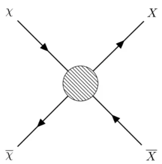
Consider a DM type of particle together with its anti-particle . We assume that the particles are stable enough so that annihilation or inverse annihilation is the process that a↵ects the number density in a comoving volume. As seen in Fig. 2.1, consider an annihilation process such as

! XX, (2.34)

where X is any SM particle the DM is allowed to annihilate into. Thermal equi-librium between the particles species is maintained as long as the interaction rate is greater than the expansion rate of the Universe. The factor (f1f2 f3f4) in

Eq. (2.31) becomes (f f¯ fXf_X¯) and the delta function ensures that E + E¯ =

EX + E_X¯. If we assume that X and X obeys Boltzmann statistics and are in

thermal equilibrium, we can write the factor as (f f¯ fEqfEq¯ ), where fEq is

the equilibrium density function. This allows us to define a quantity called the thermally-averaged cross section as

⌦ ¯!X ¯XvMøl↵= nEq 2Z d⇧1 Z d⇧2 Z d⇧3 Z d⇧4(2⇡)4 ⇥ (4)(P1+ P2 P3 P4)|M|2exp(E /T ) exp(E¯/T ), (2.35)

where we have used the expression for the number density n as in Eq. (2.12). In the above, _{¯!X ¯X} is the total annihilation cross section, summing all possible

2.3. Freeze out 23

Figure 2.1: Feynman diagram for the process _{! XX, where the blob represent} the unspecified interaction.

annihilation channels, and vMøl is the absolute value of the Møller velocity, defined

as vMøl = [|v1 v2| v1⇥ v2]1/2 =  p1 E1 p2 E2 p1 E1 ⇥ p2 E2 1/2 , (2.36) to ensure that the quantity vMøln1n2 is Lorentz invariant. When there is no

con-fusion, we can drop the subscript and simply write v for the Møller velocity. If we now scale out the expansion, as shown in the previous section, the Boltzmann equation can be written as

dY dx = xs H(m) ⌦ ¯!X ¯Xv ↵ Y2 Y_Eq2 . (2.37)

The expression for the equilibrium function YEq for cold relics is found in standard

literature [48], and is simply YEq = 45 2⇡2 ⇣ ⇡ 8 ⌘1/2 _gDM g_⇤s x 3/2_e x ⇡ 0.145g_gDM ⇤s x3/2e x. (2.38)

In the above, gDM is the degrees of freedom for the DM particles and g⇤s is the

number of relativistic degrees of freedom for the entropy density, defined as g_⇤s = X i=bosons gi ✓_T i T ◆3 + X i=fermions gi 7 8 ✓_T i T ◆3 . (2.39)

For most of the history of the Universe all particle species had a common tem-perature, and for this interval g_⇤s can be approximated as g_⇤. In the early epoch,

all SM particles were relativistic, and with the values in Tab. 2.2 we find that g_{⇤⇡ g⇤s⇡ 100.}

In order to extract some physical properties out of this Boltzmann equation we can rewrite it in a more suitable fashion. If we define the quantity

A = nEqh Avi (2.40)

as the annihilation rate, and remember that H(m) = x2H(T ), we instead obtain x YEq dY dx = A H(T ) Y2 Y2 Eq 1 ! . (2.41)

The interpretation of this expression is now much clearer. We see that as long as the annihilation rate is larger than the Hubble rate, the annihilation process is very efficient and the density function follows the equilibrium value closely. When the ratio falls below order unity, the Universe expands faster than particles can find a partner to annihilate with, and annihilation stops. This phenomenon is called freeze out, and the number of DM particles present when this occurs make up the DM abundance.

The number density is related to the matter density by multiplication of the particle mass ⇢ = m s Y . Thus, we can obtain a value for the DM density parameter

⌦DM = ⇢DM ⇢c = ms0Y0 ⇢c , (2.42)

where the zero in the subscript stands for the present value today. Data from the Planck experiment [14] tells us that ⇢c = 1.05·10 5GeV/cm 3 and s0 ⇡ 2890 cm 3,

so we obtain ⌦DM = 2.75· 108 ⇣ m GeV ⌘ Y0. (2.43)

In the end, the problem boils down to finding a model that predicts a value for ⌦DM that agrees with the experimental value seen in Tab. 2.1.

No analytic solution to Eq. (2.37) exists, but rough estimates can be made for the behaviour before and after the freeze out temperature xf. From the discussion

above we can write

Y (x < xf)⇡ YEq, Y (x > xf)⇡ Y (xf). (2.44)

For cold, i.e., non-relativistic DM, the function YEq falls o↵ exponentially before

the freeze out. After freeze out occurs, the abundance is then larger than YEq and

the di↵erence increases with x. For larger x we find dY

dx '

h vis H(m)x2Y

2_{, (2.45)}

which has the analytic solution

Y _{' x}f

H(m) h vis0

2.3. Freeze out 25 By taking_{h vi ⇠ ↵}2_/m2_{, where ↵ is the dark fine-structure constant, x}

f ⇠ 10, and

the value for the entropy today, we find ⌦DM ' 0.3 ✓ 0.01 ↵ ◆2⇣ m 100 GeV ⌘2 . (2.47)

We notice that by choosing ↵ to be of the order of 10 2 _{and the DM particle}

mass to be of the order 100 GeV, we can obtain the correct abundance observed by the Planck experiment, see Tab. 2.1. This coincidence is known as the “WIMP miracle”, as a particle with a mass at the weak scale, interacting via the Z boson, would miraculously explain DM and truly be “weakly” interacting. This is of course based on the assumption that ↵_{⇠ 10} 2_{, so by allowing ↵ to take a wider range of}

values we also open up the possibility for a wider range of masses. This is precisely the case in a few supersymmetric models [80], where the DM candidates can have a mass of several magnitudes of TeV. The word “miracle” is therefore somewhat misleading.

Since the analytic expression above only gives us a rough estimate we can use numerical methods to solve Eq. (2.37). In Fig. 2.2, we see the qualitative behaviour of the numerically integrated solutions, again, assuming that _{h vi ⇠ ↵}2_/m2_{. The}

details concerning the numerical methods used here will be handled in greater detail in the next chapter.

2.3.2

Cross sections

Calculating the thermally-averaged cross section from the definition in Eq. (2.35) is not very practical. Luckily, one can use Boltzmann statistics and, as shown in Ref. [81], find that a more useful expression to substitute for Eq. (2.35) is

⌦ ¯!X ¯Xv ↵ = 1 8m4_{T K}2 2(m/T ) Z 1 4m2 (s 4m2)psK1(ps/T )ds. (2.48)

In the above, is the annihilation cross section and s = 2m2+ 2E1E2 2p1· p2,

where m is the DM mass, and E1, E2, p1, p2 are the energies and momenta of the

two incoming DM particles. In addition, Ki is the modified Bessel function of order

i. The remaining part of this discussion will keep following Ref. [81] closely.

In theory, one can obtain the thermally averaged cross section straight from Eq. (2.48) through numerical methods. However, the behaviour of the Bessel func-tions can be hard to deal with numerically, so we are going to explore a di↵erent route. Consider an arbitrary primed frame, we define the thermally average cross section as h vMøl0 i0 = R v_Møl0 dn0₁dn0₂ R dn0 1dn02 , (2.49)

where we put a prime on the brackets to emphasize that it is averaged in that particular frame. The numerator is Lorentz invariant because of the way we define

101 102 -30 -25 -20 -15 -10 -5 0 5 = 10-2 = 10-3 = 10-1

Figure 2.2: Solutions to Eq. (2.37) where _{h vi = ↵}2_/m2_{, m = 100 GeV and ↵}

2.3. Freeze out 27 vM øl, while the denominator is not. However, as shown in Ref. [81], we find the

relation

h vMøli = h vlabilab, (2.50)

where vlab = |v1,lab v2,lab| is the relative velocity in the rest (lab) frame of one

of the incoming particles. The first average in Eq. (2.50) is thus carried out in the cosmic coving frame while the latter is averaged in the lab frame, which we will see, can be convenient. Let us now express our integral in a new parameter ", defined as the kinetic energy per unit mass in the lab frame

" = (E1,lab m) + (E2,lab m)

2m =

s 4m2

4m2 . (2.51)

The velocity expressed in this parameter becomes vlab = 2

p

"(1 + ")/(1 + 2") (2.52) and Eq. (2.48) can be written as

h vi = Z 1

0

d"_{K(x, ") v}lab, (2.53)

where _{K(x, ") is the thermal kernel, defined as} K(x, ") = _K2x2 2(x) p "(1 + 2")K1(2x p 1 + "), (2.54) and where x = m/T as before. Furthermore, for a two-particle final state we find that vlab = 1 (8⇡)2_{(s 2m}2₎ Z d⌦_|M|2, (2.55) with defined as = ✓ 1 (m3+ m4) 2 s ◆1/2✓ 1 (m3 m4) 2 s ◆1/2 . (2.56) In the above, m is the mass of the incoming particles, m3 and m4 are the masses of

the outgoing particles, and_{M is the amplitude matrix for the annihilation process.} Away from thresholds and resonance e↵ects, Eq. (2.53) can be expanded in a power series [81] of ", or alternatively x 1, as h vi = a0 + 3 2a1x 1₊  9 2a1+ 15 8 a2 x 2 · · · , (2.57) where the coefficients ai are to be explained shortly. In a similar fashion, it is also

possible to obtain a non-relativistic version of Eq. (2.53) as h vi = 2x 3/2 p_⇡ Z 1 0 vlab"1/2e x"d". (2.58)

Again, expanding this as a power series yields h vi = a0 + 3 2a1x 1₊ 15 8 a2x 2 · · · . (2.59) Comparing the expansions, i.e., Eq. (2.57) and Eq. (2.59), we see that the series coincide up to order x 1_.

When calculating cold DM abundances, it is sufficient to keep up to order x 1 terms only, since the contribution from the higher order terms are negligible [81]. This is an intuitive result because, in the language of partial waves, the first and second terms in the expansion above correspond to s-wave and p-wave annihila-tion respectively, which should dominate at low velocities. This can be realized by looking at the scattering relation l = bp [82], where l is the angular momentum quantum number, b is the impact parameter, and p is the momentum of the incom-ing particle. For slowly movincom-ing particles to have large angular momentum, they must also have large impact parameters. However, in classical scattering theory, the particles with impact parameters larger than the e↵ective range of the potential they interact with pass by una↵ected by it. This result carries over to quantum scattering theory, where only the first few partial waves needs to be considered, and where the higher partial waves are essentially una↵ected by the potential. In the simplest situation one includes only the s-wave contribution, but in some cases this term can be highly helicity suppressed, which means that p-wave annihilation dominates.

So far, little has been said about the coefficients an in the series above. These

can be obtained from Eq. (2.55) by taking the nth derivative and evaluating at " = 0 [81]; an = @n @"n ✓ 1 (8⇡)2_(4m2_{" + 2m}2₎ Z d⌦_|M|2 ◆ "=0 . (2.60) Thus, we have found a way to improve the simple estimate _{h vi ⇠ ↵}2/m2 used in the previous section. In the series expansion above, the details about the particle content at hand is encoded in the amplitude _{M, which can be calculated from the} Feynman rules to the corresponding theory.

Chapter 3

Inelastic dark matter

3.1

Motivation

There are good reasons to consider self-interacting DM models and, in particular, inelastic models. Before we move on and introduce the inelastic framework used in this thesis, we are briefly going to address some of these reasons.

3.1.1

The small scale structure problems with

self-interacting DM

It is interesting to explore if self-interacting DM can provide a solution to the small scale structure problems discussed in Sec. 1.2.2. By allowing the DM particles to scatter o↵ each other, the particles in the inner region of the DM halo can gain momentum when struck by particles falling in from the outer regions. The result is that the density profile flattens out around the center and the halo becomes more cored. This might not only provide a natural solution to the cusp-core problem, but also possibly the too-big-too-fail problem. The idea is as follows. Recall, from Sec. 1.1.2, that the rotational velocity of the stars at some radius r, is fully determined by the amount of matter M (r) enclosed by a sphere with the same radius. If the DM halo density profile is flatted out in the central region, M (r) would decrease and this would reduce the rotational velocity of the stars. Thus, it might be the case that the dwarfs we observe really are hosted by the largest subhalos, but the rotation curves are brought down by self-interactions. These e↵ects have been simulated for various models, e.g., see Refs. [83–86], and in order for the simulations to agree with observations, the cross sections (per unit mass) needs to be in the order of

m ⇠ 1 cm

2_{/g. (3.1)}

However, while the previous discussion might seem promising in the small scales, the self-interacting DM still needs to be consistent with what we observe on the

large scales. There are several ways to deduce bounds on the cross sections from the larger scales, see e.g., Refs. [87, 88], but in order to keep the discussion rather short, we highlight a particular method in what follows.

Since we know that the DM halos in galaxy clusters, such as the Bullet Cluster, pass through each other in a collisionless manner [89], the DM cannot self-interact too strongly. As discussed in Sec. 1.1.4, the density profiles of these galaxy clus-ters can be mapped out from the information obtained from gravitational lensing observations. This can be used, together with the optically observed dynamics of the clusters, to place bounds on the DM self-interaction cross sections [90, 91]. The results from this method, combined with the result from the other methods, point towards cross sections of order

m & 1 cm

2_{/g. (3.2)}

However, a more recent study suggest that the techniques used to place the tightest bounds were flawed, and that the bounds should be slightly relieved [92]. Nev-ertheless, the estimated bounds on the cross sections obtained from large scale observations are generally considered to be inconsistent with simulations.

One way to solve the small scale structure problems while avoiding the bounds from the galaxy clusters is to introduce a velocity-dependent cross section [93]. The idea is that a long range potential, such as a Yukawa potential, can boost the cross sections at the scale of dwarfs (v _{⇠ 10 km/s) while keeping them small at} the scale of clusters (v _{⇠ 1000 km/s). N-body simulations show that cross sections} generated by Yukawa-like interactions indeed reproduce the desired behaviour in dwarf halos [94]. Thus, the models to look for, which can reproduce this behaviour, are the ones where Yukawa interactions arise. It turns out, that models with light mediators are perfect candidates for this [95, 96].

A problem, however, with light mediator particles, arises if one tries to calculate the abundance through the freeze out mechanism. As discussed in Ref. [49], if the mediators are stable their comoving number density is

Ymediator ' 7 ⇥ 10 2⇠3, (3.3)

where ⇠ is the temperature ratio of the dark sector to the SM sector. By comparing this with the baryon number density YBaryon ⇠ 10 10 [48], we find that the

medi-ators can easily dominate the energy, and even overclose the Universe, unless ⇠ is small enough. However, ⇠ can not be arbitrary small because DM particles have to be populated in the thermal bath in the dark sector. The simplest way to evade the overclosure problem is to require the light mediators to be unstable, and in or-der to not interfere with the Big Bang nucleosynthesis (BBN), they need to decay into SM particles before BBN takes place. However, in the kinetic mixing case the tight bounds on the mixing pararmeters from direct detection experiments make it hard to explain the short lifetime of the mediators [49, 97]. This is because the same mixing parameters that appears in scattering processes between DM and SM particles, also appears, and suppresses, the cross sections for the decay processes.