Experimental and Mathematical Study of
Incompressible Fluid Flow through Ceramic Foam
Filters
Shahin Akbarnejad
Licentiate Thesis
Division of Applied Process Metallurgy
School of Industrial Engineering and Management
Department of Materials Science and Engineering
KTH Royal Institute of Technology
SE-100 44 Stockholm
Sweden
Akademisk avhandling som med tillstånd av Kungliga Tekniska Högskolan i Stockholm, framlägges för offentlig granskning för avläggande av Teknologie Licentiatexamen, 18 mars 2016, kl 14.00 i Sefström (M131), Brinellvägen 23,
Kungliga Tekniska Högskolan, Stockholm.
ISBN 978-91-7595-877-4
Shahin Akbarnejad Experimental and Mathematical Study of Incompressible Fluid Flow through Ceramic Foam Filters
Division of Applied Process Metallurgy
Department of Materials Science and Engineering School of Industrial Engineering and Management KTH Royal Institute of Technology
SE-100 44 Stockholm Sweden
ISBN 978-91-7595-877-4
ABSTRACT
Ceramic Foam Filters (CFFs) are widely used to filter solid particles and
inclusions from molten metal in metal production, particularly in the
aluminum industry. In general, the molten metal is poured on the top of a
ceramic foam filter until it reaches a certain height, also known as metal
head or gravity head. This is done to build the required pressure to prime
the filter media and to initiate filtration. To predict the required metal
head, it is necessary to obtain the Darcy and non-Darcy permeability
coefficients of the filter. The coefficients vary upon filter type. Here, it is
common to classify CFFs based on grades or pore per inches (PPI). These
CFFs range from10 to100 PPI and their properties vary in everything from
cell and window size to strut size. The 80-100 PPI CFFs are generally not
practical for use by industry, since the priming of the filters by a
gravitational force requires an excessive metal head. However, recently a
new method has been developed to prime such filters by using
electromagnetic Lorentz forces. This allows the filters to be primed at a
low metal head.
To continue the research work, it was deemed necessary to measure the
pressure gradients of single and stack of commercial alumina ceramic
foam filters and to obtain the permeability characteristics. Therefore,
efforts have been made to validate the previously obtained results, to
improve the permeametry experimental setup, and to obtain Darcy and
non-Darcy permeability coefficients of single 30, 50, and 80 PPI filters
and stacks of filters. Furthermore, the experimentally obtained pressure
gradients were analyzed and compered to the mathematically and
analytically estimated pressure gradients.
The studies showed that, in permeametry experiments, the sample sealing
procedure plays an important role for an accurate estimation of the
permeability constants. An inadequate sealing or an un-sealed sample
results in an underestimation of the pressure drop, which causes a
considerable error in the obtained Darcy and non-Darcy permeability
coefficients. Meanwhile, the results from the single filter experiments
showed that the permeability values of the similar PPI filters are not
identical. However, the stacks of three identical filters gave substantially
the same measured pressure drop values and roughly the same Darcy and
non-Darcy coefficients as for the single filters.
The permeability coefficients of the filters are believed to be best defined
and calculated by using the Forchheimer equation. The well-known and
widely used Ergun and Dietrich equations cannot correctly predict the
pressure drop unless a correction factor is introduced. The accuracy of the
mathematically estimated pressure drop, using COMSOL Multiphysics®
5.1, found to be dependent on the drag term used in the
Brinkman-Forchheimer equation. Unacceptable error, as high as 84 to 89 percent for
the 30, 50 and 80 PPI single filters, compared to the experimentally
obtained pressure gradient values were observed when the literature
defined Brinkman-Forchheimer drag term was used. However, when the
same second order drag term (containing the non-Darcy coefficient) as
defined in the Forchheimer equation was used, the predicted pressure
gradient profiles satisfactorily agreed with the experiment data with as
little as 0.3 to 5.5 percent deviations for the 30, 50 and 80 PPI single
filters.
Keywords: Ceramic Foam Filter, Alumina CFF, Porous Media,
Brinkman, Forchheimer, Filtration, Permeability
Acknowledgements
I wish to express my deepest gratitude to Professor Pӓr Göran Jönsson for
his endless support and providing me a possibility to fulfil my studies at
this level. I also wish to thank Professor Ragnhild Elizabeth Aune for
introducing the subject and giving me a chance to enhance my skills. I
would like to thank Professor Du Sichen and Professor Malin Selleby for
the opportunity to finalize my studies.
I am also grateful for the technical reviews and guidance provided by Dr.
Mark William Kennedy and Dr. Lage Tord Ingemar Jonsson.
I wish to express gratitude to Mr. Egil Torsetnes at NTNU for helping
with construction of the experimental apparatus.
I am also thankful to my colleagues and friends at both NTNU and KTH
Universities who have assisted me at various times, particularly to Robert
Fritzsch and Mohsen Saffari Pour.
Last but not least, I would like to thank my wife Mansoureh Shahsavani
for her boundless support and allowing me the opportunity to apply
myself to the task.
The funding and support by the Swedish Steel Producers Association
“JERNKONTORET” and the laboratory and technical supports from the
materials science departments at NTNU and KTH are also acknowledged.
Supplements
The present thesis is based on the following supplements:
Supplement I:
An Investigation on Permeability of Ceramic Foam Filters (CFF)
Shahin Akbarnejad, Mark William Kennedy, Robert Fritzsch, and
Ragnhild Elizabeth Aune
Light Metals 2015, pp. 949-954.
Supplement II:
Analysis on Experimental Investigation and Mathematical Modelling of
Incompressible Flow through Ceramic Foam Filters
Shahin Akbarnejad, Lage Tord Ingemar Jonsson, Mark William Kennedy,
Ragnhild Elizabeth Aune, and Pӓr Göran Jönsson
Submitted to Metallurgical and Materials Transactions B, 2016
Supplement III:
Significance of Fluid Bypassing Effect on Darcy and Non-Darcy
Permeability Parameters of Ceramic Foam Filters
Shahin Akbarnejad, Mohsen Saffari Pour, Lage Tord Ingemar Jonsson,
and Pӓr Göran Jönsson
The contributions of the author to different supplements of the thesis:
Supplement I: Literature review, designing the experiments,
experimental work, data analysis, and writing the manuscript.
Supplement II: Literature review, designing the experiments,
experimental work, computational fluid dynamics simulations, data
analysis, and writing the manuscript.
Supplement III: Literature review, designing the experiments,
experimental work, computational fluid dynamics simulations, data
analysis, and writing the manuscript.
Papers as second or third author which are not included in the thesis:
1. Effect of Electromagnetic Fields on the Priming of High Grade Ceramic
Foam Filters (CFF) with Liquid Aluminum
Robert Fritzsch, Mark William Kennedy, Shahin Akbarnejad and
Ragnhild Elizabeth Aune
Light Metals 2015, pp. 929-935. (Received the 2015 TMS Light Metals
Subject Award)
2. A Novel Method for Automated Quantification of Particles in Solidified
Aluminum
Robert Fritzsch, Shahin Akbarnejad and Ragnhild Elizabeth Aune
TMS 2014 Supplemental Proceedings, pp.535-543
Presentation
An Investigation on Permeability of Ceramic Foam Filters (CFF)
Shahin Akbarnejad, Mark William Kennedy, Robert Fritzsch, and
Ragnhild Elizabeth Aune
Cast Shop for Aluminum Production, 2015 TMS Annual Meeting &
Exhibition, March 15-19, Orlando, Florida
TABLE OF CONTENTS
1 INTRODUCTION
1
2 MEHTODOLOGY
5
2.1 Permeametry Experiments
5
2.1.1Sample preparations 6
2.1.2 Measurement devices 9
2.1.3 Experimental procedure 9
2.1.4 Obtaining the Darcy and non-Darcy coefficients 10
2.2 Estimating pressure drop based on filter physical properties 11
2.3 Mathematical modelling
12
2.3.1 Reynolds number 14
2.3.2 Assumptions 14
2.3.3 The transport equations 15
2.3.4 The Reynolds-averaged Navier-Stokes equations 16
2.3.5 The Algebraic equation 17
2.3.6 The Brinkman-Forchheimer equation 17
2.3.7 Boundary conditions and mesh quality 19
3 RESULTS 21
3.1 Permeametry experiments 21
3.2 Darcy and non-Darcy permeability coefficients 25
3.3 Estimating pressure drop from filter physical properties 26
3.4 Mathematical modelling 30
3.4.1 Mesh sensitivity study 33
3.4.2 Influence of the Drag term 34
3.4.3 Significance of the sealing 40
4 DISCUSSIONS 43
4.2 Estimating pressure drop from filter physical properties 48
4.3 Computational fluid dynamics 51
4.3.1 Influence of the drag term 51
4.3.2 Significance of the sealing 54
5 CONCLUSIONS 56
6 FUTURE WORKS 59
1 INTRODUCTION
Ceramic Foam filters (CFFs) have been widely used in various industries, i.e. in the petrochemical sector, automotive industry and metallurgical field, to remove, control or reduce the quantity of the unwanted substances. In metallurgy and particularly in the aluminium industry, CFFs have been used to filter solid inclusions from molten metal for decades. These non-metallic inclusions can be aluminium oxides, refractory particles, spinels, magnesium oxides, borides, nitrides, and carbides. Such impurities have negative effects on processing, mechanical properties, and surface quality of the products made from aluminium [1]–[7].
Ceramic foam filters can either be open cell or closed cell materials. Each category has a different structure, property and application[8]–[10]. Ceramic foams have sufficiently high mechanical properties, i.e. high thermal and chemical resistance, and high structural uniformity and strength, depending on the type and production method [10].
The open cell CFFs possess a porous structure of voids shaped by a web or ‘mesh’ of a ceramic material [4]. These CFFs are classified in different grades or PPIs (Pore Per Inch). Therefore, the physical properties of the filters: porosity, tortuosity, and pore, window and strut size vary with grade or the PPI. Such differences have an influence on the priming and permeability of the filters [2], [6], [11].
In order to filter molten metal, the melt is poured on the top of a filter. To initiate the filtration it is essential to prime the filter. Here, priming can be defined as filling the filter with molten metal and removing the entrapped air. Thus, for the melt to flow through the filter it has to reach a required height to build a certain level of pressure (gravity head) to prime the filter.
To predict the pressure drop of a CFF at a given melt flow rate, the permeability characteristics of the filter must be studied. Permeability is the ability of a CFF or such media to let a fluid, i.e. liquid metal, to pass through its pores and openings. In general, the permeability characteristics can be determined in two ways: (i) performing permeametry experiments and (ii) estimating by physical properties of the filter media using formulas from the literature, i.e. calculating the pressure gradient from the literature defined equations, which use the cell, window and strut sizes of the filter. In this research work both methods have been explored to obtain the permeability parameters and to make a comparison of the findings. In addition, mathematical modelling, i.e. Computational Fluid Dynamics simulations (CFD), using COMSOL Multiphysics® 5.1 were also applied to verify and compare the results to the experimental findings.
The permeametry experiments are used to measure the pressured drop as a function of superficial velocity. To estimate the Darcy k1 [m2] and non-Darcy k2 [m] permeability coefficients, it is very common to use Forchheimer equation (Eq.1) for incompressible fluids. The coefficients can be calculated using Eq.1 by knowing the pressure drop ∆P [Pa], filter thickness L [m], superficial velocity Vs [m/s], dynamic viscosity µ [Pa·s], and the fluid density ρ [kg/m3] [2], [6], [12]– [14]. 2 1 2 s s P V V L k k
(Eq.1)
The key point in this approach is to avoid fluid bypassing. It has been stated in the literature [6], [15]–[28] that fluid bypassing from the gap between the filter and the filter holder during permeametry results in an underestimation of the pressure gradient. This consequently causes an underestimation in the obtained Darcy and non-Darcy permeability coefficients.
Several formulas have been suggested in the literature [29], [30] to estimate the pressure drop and permeability characteristics from the filter physical properties. The formulas use cell, window or strut sizes of the filter matrix. The most common and well-known correlation is the Ergun equation (Eq.2) for fluid flow through beds of granular solids [31]. The equation estimates the pressure drop ∆P when the rest of the parameters such as; porosity ɛ [unit less], the equivalent Spherical particle diameter dp [m], filter thickness L [m], superficial velocity Vs [m/s], dynamic viscosity µ [Pa·s], and the fluid density ρ [kg/m3] are known. The equivalent spherical particle diameter (dp) is defined (Eq.3) as specific surface (Sv), the surface of solids per unit volume of solids.
2 2 3 2 3 (1 ) (1 ) 150 s 1.75 s P P P V V L d d
(Eq.2) 6 P v d S (Eq.3)The correlation (Eq.2) has been broadly investigated since 1951, when it was first introduced by Ergun. Over the years, many scientists have presented optimized versions of the equation. However, even the optimized versions show a ±50 percent deviation when the estimated values are compared to the experimental results [32], [33]. Originally, the empirical Ergun equation had been adopted for columns of packed beds. Therefore, there seems to be some confusion in the literature when introducing the equivalent spherical particle diameter (dp) as the pore size in ceramic foam filters in the Ergun equation. Some researchers used the cell diameter and others considered the window diameter to explore the correlation [34], [35].
An optimized version of the Ergun equation was suggested by Dietrich [14]. The equation (Eq.4) uses hydraulic diameter (dh) to estimate the pressure drop. The hydraulic diameter was associated with specific surface (Sv) and porosity (Eq.5). The specific surface can be measured directly via Magnetic Resonance Imaging
(MRI) or it could be estimated based on the theoretical correlation (Eq.6) introduced by Buciuman [36], [37]. Although Ergun’s and Dietrich’s specific surface may have the same notation (Sv), the definitions seem to be different.
2 2 2 110 s 1.45 s h h P V V L d d
(Eq.4) 4 h v d S (Eq.5) 1 (1 )n v s w S C d d (Eq.6)where the parameters (ds)and(dw)arethe strut and window diameters of a ceramic foam filter, C and n are the equation constants. The C and n constants were stated to have the values of 4.82 and 0.5 for a Tetrakaidecahedron and were experimentally determined to be 2.87 and 0.25 in real sponges [14], [37]. Later, Dietrich studied the correlation (Eq.4) more in-depth and found that the equation is satisfactorily capable of modelling 2500 data point values from the literature with a ± 40 percent accuracy [17].
Recently Kennedy and et al. suggested an Ergun-type correlation (Eq.7) based on experimental measurements on commercial alumina ceramic foam filters of 30, 50, and 80 PPI. The deviations to the experimentally obtained data was reported to be in the range of 30 to 40 percent [6].
2 2 3 2 3 (1 ) (1 ) 8.385 150
(
s 1.75 s)
w w P V V L d d (Eq.7)2 MEHTODOLOGY
2.1 Permeametry Experiments
The liquid permeability characteristics of 50 millimetre thick commercial alumina ceramic foam filters with 30, 50 and 80 PPI were studied using water as the working fluid in liquid permeametry. Specifically, two Plexiglas® filter holders were fabricated and used; one for single filter experiments and one for triple filter experiments. Figures 1 and 2 shows a sketch of the experimental setup for pressure drop measurements of the single filters and stack of three filters. Ordinary tap water in the temperature range of 282 K to 284 K (9ºC to 11ºC) was circulated through a smooth pipe, with ~50 mm external diameter or ~48 mm internal diameter, with mass flow rates in the range of 0.62 to 1.74 kg/s.
Figure 2: Pressure drop measurement apparatus for stacks of 3 filters
2.1.1 Sample preparations
A series of nine ~51 mm diameter samples were cut from standard commercial 9 inch 30, 50 ,and 80 PPI alumina filters using a Computer Numerical Control (CNC) water jet machine, as shown in Figure 3A. To be specific, (3) 30 PPI, (3) 50 PPI, and (3) 80 PPI samples were prepared. The samples were cut about 1mm larger than the internal diameter of the filter holder. This was done to create a margin to avoid any bias in the sample size and to fabricate an equal gap, between the outer surface of the samples and the inner diameter of the filter holder, for the sealing procedure. The significance of sample sealing in permeametry studies has been mentioned in the literature [6], [15]–[28]. Therefore sealing procedure was applied to prevent fluid bypassing from the gap between the filter and the filter holder. No sealing or inadequate sealing is believed to result in fluid bypassing which causes underestimation of the pressure gradient and consequently to an
underestimation of the Darcy (k1) and non-Darcy (k2) permeability coefficients[6], [15]–[28].
The sealing procedure contains three steps: (i) blocking the side walls of the samples, (ii) resizing and (iii) wrapping in grease impregnated cellulose fibre. The combination of cellulose fibre and grease is essential to tighten the samples, while fitting them into the filter holder. Figure 3B shows sealed samples that were fitted into the sample holders. All nine samples used in permeametry experiments were taken from the corner of the 9 inch 30, 50, and 80 PPI filters, as shown in Figure 2A. Also, exactly the same sample preparation procedure was applied to all samples.
Figure 3: A) 9 inch 50 PPI filter with samples taken from the filter B) samples sealed and fitted into the sample holders[16]
In order to calculate the filter porosity, the samples were first dried in an oven at 150°C for 15 hours. Then, they were resized to fit into the filter holders. Once they fit into the filter holder the samples were taken out for dimension measurement. Here, the height and diameter of the samples were measured by a digital calliper with an accuracy of 0.03 mm and a resolution of 0.01 mm. Later, the samples were weighed using a digital laboratory scale with a resolution of
0.01 g. The theoretical volumes of the samples were calculated based on the dimensions of the samples. Then, the theoretical weight was estimated by considering the density of the CFF, which was obtained from the manufacturer, 3.48 [g/cm3]. Also, the actual volume was measured using a series of graduated cylinders [16].
The total and open pore porosities of the filters were calculated based on weight (Eq.8) and volume (Eq.9). Here, the open pore porosity is the total porosity excluding the trapped porosity. The trapped porosities are the void space inside of struts and the micro-porosity of the filter media. The difference in the porosity values are expected to be less than 5 percent in alumina CFFs [6], [17], [38]. The results of the dimension and porosity measurements are shown in Table 1. The recorded diameter and thickness values represent the average values of ten readings with a confidence interval of 95 percent.
- 100 Mt Ma Total Porosity Mt (Eq.8)
-
100 Vt VaOpen Pore Porosity
Vt
(Eq.9)
where Mt is the theoretical weight [g], Ma the measured weight [g], Vt the theoretical volume [mm3] and Va the measured volume [mm3].
Table 1: Filter dimensions and porosities[16]
Filter Diameter [mm] Thickness [mm] Total porosity [%] Open pore porosity [%] No. Type N1 30 PPI 49.33 ± 0.30 50.42 ± 0.07 90 88.8 N2 30 PPI 49.00 ± 0.37 50.83 ± 0.04 91 90 N3 30 PPI 49.38 ± 0.14 50.76 ± 0.06 90 91.5 N1 50 PPI 49.58 ± 0.18 50.88 ± 0.05 86 83.5 N2 50 PPI 49.30 ± 0.17 49.98 ± 0.02 86 84.6 N3 50 PPI 49.68 ± 0.10 50.63 ± 0.06 85.9 82.6 N1 80 PPI 49.63 ± 0.15 49.79 ± 0.04 85.6 81.5 N2 80 PPI 49.38 ± 0.28 50.28 ± 0.03 86.4 85.8 N3 80 PPI 49.30 ± 0.15 50.96 ± 0.06 87 85.1
2.1.2 Measurement devices
The fluid pressure before and after the filter samples were obtained using a DF-2 (AEP, Transducer, Italy) pressure transducer. The device has a measuring range from 0 to 1 bar, an output range of 4 to 20 mA DC, and a certified error of ‹±0.04% of reading according to the factory calibration. The current produced by the pressure transducer was measured using a FLUKE 289/FVF true-RMS digital multi-meter. The multi meter has a data logging feature and a resolution of 0.01 µA, when using a DC current[16].
The water velocity was calculated based on the mass flow measured during a specified time period using the weight gain in a container with a maximum capacity of 53 kg of water. To measure and log the gain-in-weight, an OHUAS T31P scale (3000 series indicator) equipped with an OHAUS Data Acquisition Software (D.A.S.) was used. Also, the temperature was monitored and measured using a FLUKE 80PT-25 T-Type probe with an accuracy of ±1°C in the temperature range of 0°C to 350°C. The temperature data was logged by a National Instruments NI USB-TC01 logger. Furthermore, the data were collected at one second intervals for all three logging devices[16].
2.1.3 Experimental procedure
Samples were divided into three groups, N1-N3, and all were sealed before the permeametry experiments, according to the sealing procedure. In addition, the N3 group was initially used as a benchmark sample where no sealing procedure was applied. This allowed for an unhindered bypassing of the fluid along the wall of the filter holder apparatus. After performing experiments with the un-sealed and well-sealed single filters using the single filter apparatus, a series of stack of three filters were measured. In this series of experiments three filters and filter holders were used, as shown in Figures 1 and 2. During the experiments; samples from group 1 (N1) were always kept as the ones facing the inlet of the apparatus. Also,
Group 2 Samples (N2) in the middle and Group 3 (N3) were always placed at the end or were faced towards the outlet of the apparatus[16].
The water flow was produced by a 1000 W submersible pump with maximum 0.8 bar pressure limit. The pump was placed at the bottom of a 53 kilograms capacity container. A DN 25 ball valve was used to regulate the flow. The valve was located between the outlet of the pump and the inlet of the experimental setup pipeline. A straight inlet pipe length of 1.2 m or about 25 L/D’s before the inlet of the pressure measuring apparatus was used, to enable the flow profile to develop. Also, a similar length of straight pipe was used after the apparatus. Previous permeametry studies revealed no significant influence by using a longer inlet length on the measured pressure drop [6].
The Thiesen - Scheel – Diesselhorst [39] relation (Eq.10) was used to calculate the water density at the temperature T [°C] for the experimental trails.
2 288.9414 1000 1 ( 3.9863) 508929.2 68.12963 T T T (Eq.10)Then, the water viscosity at the temperature of the experiment was calculated according to the recommended formulation by the International Association for the Properties of Water and Steam (IAPWS) for the viscosity of ordinary water [40].
2.1.4 Obtaining the Darcy and non-Darcy coefficients
The measured values of the pressure drops and fluid flow rates and the calculated values of water density and viscosity were used to estimate the Darcy (k1) and non-Darcy (k2) permeability coefficients in accordance to the Forchheimer’s equation (Eq.1). Overall, four methods were used to obtain the coefficients:
i. Polynomial interpolation: Via equations derived automatically by fitting a second order polynomial trend line using Excel 2010 with an intercept fixed at zero [16].
ii. Total least squares: A non-linear least square curve fitting technique using Excel 2010 to automatically obtain k1 and k2 values [41]. iii. Nonlinear regression: A quadratic regression using Excel 2010 at a
zero intercept.
iv. Ergun’s approach: Dividing the Forchheimer equation (Eq.1) by velocity and performing a linear regression[6], [31].
The obtained k1 and k2 coefficients were used to re-calculate the pressure drop values using the Forchheimer equation (Eq.1). Then, the least average deviation to the experimentally obtained pressure drop values was set to be the criterion for the selection of the appropriate method.
2.2 Estimating pressure drop based on filter physical properties
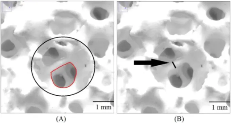
To apply and study the Ergun (Eq.2), Dietrich (Eq.4) and Kennedy equations (Eq.7); the cell, window and strut diameters of the filters were measured. For that reason, the uncut factory made surface of the 50 mm diameter samples were scanned in 2400 dpi (dots per inch) using a flatbed scanner. Then, the high quality images were processed by using the “ImageJ 1.48v” software to measure the cell, window and strut diameters. In this method, the areas of the filter cells and filter windows were manually defined as shown in Figure 4A. Then, the defined areas were automatically calculated by the software. Afterwards, the equivalent diameters were calculated in an excel sheet assuming that the measured area is the area of a circle. In strut diameter measurements, the measured strut width at the middle of the strut was assumed to be equivalent to a strut diameter, as presented in Figure 4B.Figure 4: Measurements of the equivalent cell, window, and strut diameter of a 30 PPI CFF using “ImageJ 1.48v” software: A) Cross
section of the surface of the filter with a measured cell area (black circle) and a window area (irregular red shape), and B) Strut equivalent
diameter measurement (short black line)
2.3 Mathematical modelling
To obtain pressure gradient as a function of fluid velocity using mathematical modelling, two dimensional (2D) axisymmetric 30, 50, and 80 PPI single model simulations were conducted by using the commercial COMSOL Multiphysics® 5.1 software. Later, the results were assessed and compared to the results from the experiments. In order to do this, two mathematical models were created:
i. A model representing the well-sealed condition where no gap between the filter holder and the filter were considered
ii. A model representing the un-sealed trials where the gap between the filter holder and the filter were also considered
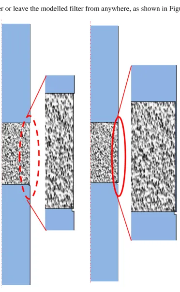
In the modelled well-sealed condition; the modelled inlet pipe section was connected to the top of the filter and the lower part of the modelled filter was connected to the outlet pipe. Thus, water could only enter the model from the top and leave from the opposite side and not leave or enter the modelled filter from the side walls, as presented in Figure 5A. On the other hand, in the modelled un-sealed condition; a gap representing the gap between the filter and filter holder
was introduced. Therefore, water was allowed to enter the sections from the top and leave from the opposite side. Furthermore, water could pass through the introduced additional space adjacent to the side walls, i.e. the gap, and would be free to enter or leave the modelled filter from anywhere, as shown in Figure 5B.
(A) (B)
Figure 5: Schematic view of the 2D axisymmetric CFD models: A) a modelled well-sealed condition, and B) a modelled un-sealed condition
The models were created according to the actual filter dimensions given in Table 1 and as illustrated in Figures 5A and 5B. In addition, the porous matrix properties and fluid properties, e.g. the Forchheimer coefficients, filter porosity; fluid density, fluid temperature, and dynamic viscosity were set according to the experimental conditions. The values are presented in Table 4 in the Results chapter.
2.3.1 Reynolds number
In order to define the fluid flow regime and to select the appropriate module in the software, the Reynolds numbers were calculated. In a pipe, the Reynolds number can be calculated using Eq.11. In the equation, D is the pipe diameter [m] and the rest are the fluid properties: ρ density [Kg/m3], velocity V [m/s], and dynamic viscosity µ [Pa·s] [42][43].
e
VD
R
(Eq.11)
The Reynolds numbers for both the well-sealed and un-sealed samples and for all 30, 50, and 80 PPI filter experiment groups were calculated. The calculations were based on the experimentally obtained average outflow fluid velocities as well as the calculated fluid densities and viscosities. The obtained Reynolds numbers for the well-sealed samples were found to be in the range of 2500-26000. The Reynolds numbers for the un-sealed samples were also in the range of 5750-32400. The turbulent flow regime begins at Re ˃ 2300 [42][43]. Therefore, the turbulent fluid flow CFD simulations were applied in this research work.
2.3.2 Assumptions
The following assumptions have been made in the statement of the mathematical model:
ii. The temperature, and the fluid density and dynamic viscosity are assumed to be constant
iii. The solution is independent of time, i.e. a stationary solution with wall initialization was used
iv. The gravitational force was not considered (because in the experiment the filters were positioned horizontally)
v. The pipe surface was considered to be smooth and frictionless vi. Turbulence was modelled based on Prandtl’s mixing length theory
2.3.3 The transport equations
To simulate turbulent flow for incompressible fluids with an added porous media domain in Comsol Multiphysics® 5.1, one may use the “The Turbulent flow, Algebraic yPlus Interface” module. It is necessary to mention that the other well-known and widely used turbulent modules, i.e. k-ɛ, k-ω etc., were not available within a porous media domain in COMSOL Multiphysics® 5.1. Therefore, the following governing transport equations for the fluid flow in the pipe section and the filter media need to be solved:
i. The Reynolds-Averaged Navier-Stokes (RANS) equations for incompressible fluids, including continuity and conservation of momentum
ii. An algebraic equation to model Turbulence
iii. The Brinkman-Forchheimer equation together with the continuity equation to model the flow in the porous domain
The equations were automatically solved by using the “The Turbulent flow, Algebraic yPlus Interface” module in COMSOL Multiphysics® 5.1 software. More specifically the governing transport equations in their general form may be expressed as follows:
2.3.4 The Reynolds-averaged Navier-Stokes equations
The turbulence regime consists of random fluctuations of various fluid flow properties in time and space, such as velocity, pressure and etc. It is believed that the available mathematic knowledge cannot handle such instantaneous fluctuations [43]. Therefore, it is very common to use the Reynold’s statistical approach to mathematically simplify the turbulent fluid flow studies[42]–[44]. Based on the Reynolds averaging approach (Eq.12), the instantaneous quantity (u) can be expressed as the sum of the average value (U) plus the fluctuating part (u′). The details of the averaging procedure can be studied in the following references [43], [44].
u
U
u
(Eq.12) The Raynolds-Averaged Navier-Stokes (RANS) equations, i.e. the continuity equation (Eq.13) plus the momentum equations (Eq.14), for incompressible fluids at steady sate and in their general form can be written as follows[43], [44]:
i
0 i U x (Eq.13) j i i j i j j i j j i U U P U U u u x x x x x (Eq.14)where ρ is density, Ui the time averaged mean velocity in xi direction and Uj the time averaged mean velocity in xj direction, P is pressure, µ is the dynamic viscosity and
i j
u u
is known as the Reynolds stress tensor (τij). The left hand side of the Eq.14 represents convection. The right hand side of the equation consists of: pressure gradient, viscous diffusion and turbulent diffusion terms. The Reynolds stress tensor (τij) is expressed as a function of eddy or turbulent viscosity (μT) [42]–[44]: ij i j T dU u u dy (Eq.15)
In RANS equations all parameters are known, i.e. pressure, velocity and etc. could be experimentally obtained, except the Reynolds stress tensor (τij) or turbulent viscosity (μT). This unknown parameter needs to be estimated or modelled. One difference between the turbulence modules is the approach towards solving the stress tensor or eddy viscosity. As explained, in this study Prandtl’s mixing length theory[43]–[45] was applied to estimate the turbulent viscosity (μT).
2.3.5
The Algebraic equation
According to L.Prandtl’s mixing length hypothesis, the eddy viscosity can be estimated as a function of the mixing length. The hypothesis assumes that a lump of fluid displacing in transverse direction maintains its mean properties for a characteristic length of lmix until it mixes with its surroundings[43]–[45].Thus, the eddy or turbulent viscosity can be expressed as follows:
2 T mix dU l dy (Eq.16)
Prandtl also assumed that the mixing length (lmix) is approximately proportional to the distance y from the wall. Here the proportionality constant is known as Kármán constant and it is assumed to be ~ 0.41[43]–[45].
mix
l
y
(Eq.17)2.3.6 The Brinkman-Forchheimer equation
The effects of the solid boundary or inertial forces on the fluid flow through a porous media are expected to be significant, especially in a high porous media [46]. Therefore a momentum equation that represents the sum of the viscous (Darcy term) and kinetic energy losses (non-Darcy term) needs to be solved[6].
In COMSOL Multiphysics® 5.1, the Brinkman-Forchheimer equation (Eq.18) is used to define the momentum equation in a porous medium[47]–[51]. The
Brinkman-Forchheimer equation is a modified version of the standard momentum equation in a pipe (Eq.14). In addition to the terms explained in Eq.14, two additional terms that represent the resistance to fluid flow in the porous media, i.e. The Darcy and non-Darcy (Forchheimer) terms, are included in the right hand side of the Brinkman-Forchheimer equation. The Brinkman-Forchheimer equation in a steady state and statistically time averaged conditions can mathematically be written as follows[47], [50], [52]–[55]:
i i j j j i j i j j i U U P U U u u x x x x x
j i j j i j i j j U U U U U u u k U U (Eq.18)where ɛ is filter porosity, k is the Darcy permeability coefficient [m2], and β is the Brinkman-Forchheimer drag coefficient [Kg/m4]. Also, based on Prandtl´s hypothesis and from Eq.15 and Eq.16 the eddy or turbulent viscosity
i j
u u
term can be calculated as follows:
2 j i mix dU u u l dy (Eq.19)
The Brinkman-Forchheimer drag term β is defined through geometric function F [dimensionless], fluid density ρ [kg/m3], ɛ porosity [dimensionless], and the Darcy permeability coefficients k [m2], as shown in Eq.20. The geometric function F can be calculated from porosity using a correlation based on Ergun’s experimental findings (Eq.21). The Darcy permeability coefficient (k) can be obtained directly from permeametry experiments or estimated by Ergun’s suggested formula (Eq.22) using the porosity (ɛ) and particle diameter (dp) [47], [48], [56]–[60].
F k
3 1.75 150 F (Eq.21)
3 2 2 150 1 p d k (Eq.22)In addition to the Brinkman-Forchheimer drag term an alternative drag term was also examined. The alternative drag term is the same second order coefficient, here labelled as βF, as in the Forchheimer equation (Eq.1). The drag term is defined by the fluid density ρ [kg/m3], and the non-Darcy permeability coefficient k2 [m] as follows: 2 F k
(Eq.23)2.3.7 Boundary conditions and mesh quality
A summary of the boundary conditions for the system is given in table II. At the inlet, no viscous stress with both the maximum applied pressure (~50 kPa gauge) and a theoretical minimum (zero gauge) inlet pressure were tested to evaluate if the inlet pressure had any impact on COMSOL’s results for an incompressible fluid. At the outlet, no slip conditions for the walls and a uniform outflow velocity were assumed. This was done to simulate the exact experimental conditions. Also, considering the tendency of porous media to reduce variation in flow velocity, it seemed more reasonable to assume a uniform outlet velocities rather than a uniform inlet velocity.
The outlet velocity values were based on the obtained experimental data. In addition to the pressure (P), the velocity field components (u) and (w) were calculated from the geometry, according to Eq.16, Eq.17, and Eq.22.
In COMSOL Multiphysics® 5.1, mesh quality is defined in the range of 0 to 1 and 0.1 is the minimum acceptable average mesh quality[48]. As a result, several
mesh types were used to calibrate the solution. It is expected to obtain the most reliable results by achieving the highest possible average mesh quality. The mesh sensitivity study details are discussed in the result chapter.
Table 2: Boundary conditions
Inlet outlet Wall
50000[ ] p Pa u U n ms0 1 u 0ms1
3 RESULTS
3.1 Permeametry experiments
After running single and stacks of three filters experiments on 30, 50, and 80 PPI alumina filters, the measured pressure drop before and after the filters and the mean fluid velocity values were used to plot pressure gradient profiles and to calculate the Darcy (k1) and non-Darcy (k2) permeability coefficients in accordance to the Forchheimer equation (Eq.1). The pressure gradient profiles [Pa/m] as a function of the superficial velocity [m/s] are shown in Figures 5-7. More specifically, the three green solid curves are pressure gradient profiles of the well-sealed single samples and the short red solid curves are pressure gradient profiles of the well-sealed stack of three filter samples. The stack three pressure gradient profile curves lay somewhere among the well-sealed single pressure gradient profiles. In addition to the well-sealed trails, the pressure gradients of the un-sealed 30, 50 and 80 PPI samples were also measured and plotted. The dotted curves in Figures 6-8 represent the pressure gradient profiles of the un-sealed samples.
In Figures 6-8, each reported data point represents an average of minimum 24, 26, and 31 readings for the 30, 50 and 80 PPI filters respectively. As a result, the minimum and maximum margins of error with a confidence interval of 95 percent is in the range of 1.3 to 6.5% for the fluid velocity values and 0.5 to 4% for the pressured gradient values of the 30, 50, and 80 PPI ceramic foam filters, as shown in Figure 9.
In addition to the current experimentally obtained pressure gradient and superficial velocity values, previous research results by Kennedy and et. al [6] are also presented in Figures 6 to 8. The blue solid curves labelled as “P” are the previous results. In the current research work, similar experimental procedures to Kennedy’s were also applied. The only differences compared to the previous
work are the following: (i) a slightly different sealing procedure was applied, (ii) the 30, 50, and 80 PPI alumina CFFs were from the same manufacturer but from a different batch, (iii) instead of a K-type thermocouple a T-type thermocouple with a measurement accuracy of ±1°C in the temperature range of 273 K to 623 K (0°C to 350°C) was used, and (iv) a multi meter with lower resolution and higher accuracy was used.
Figure 6: Measured pressure drop over filter thickness as a function of the superficial velocity of the well-sealed single (the green solid curves)
and stacks of three (the red solid curve) 30 PPI filters, an un-sealed 30 PPI sample (the dotted curve) and the previous studies [6] labelled as P
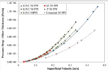
Figure 7: Measured pressure drop over filter thickness a function of the superficial velocity of the well-sealed single (the green solid curves) and stacks of three (the red solid curve) 50 PPI filters, an un-sealed 50 PPI sample (the dotted curve) and the previous studies [6] labelled as P (the
blue solid curve)
Figure 8: Measured pressure drop over filter thickness a function of the superficial velocity of the well-sealed single (the green solid curves) and stacks of three (the red solid curve) 80 PPI filters, an un-sealed 80 PPI sample (the dotted curve) and the previous studies [6] labelled as P (the
Figure 9: Measured pressure gradients of the fully sealed single 30, 50, and 80 PPI filters (the dark solid curves) as a function of the superficial velocity containing the lower and upper curves of the margins of errors
(the dotted curves). Data are given with the 95 percent confidence intervals
3.2 Darcy and non-Darcy permeability coefficients
As explained in the method chapter, four different methods were applied to calculate the coefficients. The estimated Darcy and non-Darcy permeability coefficient values from each method were used to re-calculate the pressure gradients using the Forchheimer equation (Eq.1). The re-calculated pressure gradients were compared to the experimentally obtained data. Table 3 presents the estimated Darcy and non-Darcy permeability coefficient values from each method and compares the average deviations of the re-calculated pressure gradient to the experimental data in a single 50 PPI (S1N1).
Table 3: A comparison between the calculated the Darcy (k1) and non-Darcy (k2) coefficients from four methods and the average deviations between the calculated and experimentally obtained
pressure gradients of a single 50 PPI (S1N1)
Method k1 [m2] k2 [m] average deviation* [%] Polynomial interpolation 1.489E-08 1.428E-04 9.548
Total least squares 5.682E-08 1.446E-04 1.297
Nonlinear regression 1.489E-08 1.497E-04 0.287
Ergun’s approach 1.602E-08 1.491E-04 0.226
*The average deviations between the calculated and experimentally obtained pressure gradients
The re-calculated pressure gradients using the Ergun’s approach, i.e. dividing the Forchheimer equation (Eq.1) by velocity and performing a linear regression[6],[31], provided the least average deviation to the experimentally obtained pressure gradients. Therefore, the Ergun’s approach was used to calculate the coefficients in the remaining part of this research work. Table 4 shows the calculated (k1) and (k2) values for the well-sealed single filters and for stacks of three filters. In addition, the measured water temperature and the calculated water viscosities and densities are also given.
Table 4: The empirically obtained permeability coefficients, measured water temperatures, and the estimated viscosities and densities during the experiments
Sample No Water Temperature [K] Water Viscosity [Pa s] Water Density [Kg/m3] Forchheimer k1 [m2] Forchheimer k2 [m]
N1 30 283.6 1.29E-03 999.7 3.130E-08 6.276E-04
N2 30 283.0 1.31E-03 999.7 3.430E-08 6.938E-04
N3 30 283.6 1.29E-03 999.7 3.705E-08 6.434E-04
N1 50 282.5 1.33E-03 999.8 1.602E-08 1.491E-04
N2 50 283.3 1.30E-03 999.7 2.150E-08 1.201E-04
N3 50 283.4 1.30E-03 999.7 1.961E-08 1.136E-04
N1 80 283.8 1.28E-03 999.7 5.290E-09 8.855E-05
N2 80 283.6 1.29E-03 999.7 8.540E-09 1.387E-04
N3 80 283.7 1.28E-03 999.7 8.692E-09 1.074E-04
N1N2N3 30 283.7 1.28E-03 999.7 3.668E-08 6.506E-04
N1N2N3 50 283.6 1.29E-03 999.7 1.704E-08 1.277E-04
N1N2N3 80 284.2 1.27E-03 999.6 6.429E-09 1.084E-04
In addition to the well-sealed samples, the Darcy (k1) and non-Darcy (k2) permeability coefficients of the un-sealed 30, 50, and 80 PPI samples were also calculated. Table 5 presents: (i) the empirically obtained permeability coefficients of group N3 single samples for both the well-sealed and un-sealed conditions, and (ii) compares the deviations between them.
Table 5: Calculated k1 and k2 values of the fully sealed and un-sealed single samples of Group N3
Filter type Cal. Values Sealed Sample Unsealed Sample Deviation [%] 30 PPI k1 [m 2 ] 3.705E-08 4.068E-08 8.94 k2 [m] 6.434E-04 1.577E-03 59.21 50 PPI k1 [m 2 ] 1.961E-08 2.446E-08 19.83 k2 [m] 1.136E-04 2.696E-04 57.85 80 PPI k1 [m 2 ] 8.692E-09 1.258E-08 30.88 k2 [m] 1.074E-04 2.893E-04 62.88
3.3 Estimating the pressure drop from filter physical properties
A semi-automatic technique, which is explained in the Method chapter, was used to obtain the equivalent cell, window, and strut diameters of 30, 50, and 80 PPI alumina CFFs. The presented equivalent diameters in Table 6 are the averagevalues of 60, 200, and 80 readings respectively for each PPI filter. Moreover, the reported average and margin of error data are with 95 percent confidence intervals. In addition, histograms made of 200 counts of the window diameter (dw) size distribution for 30, 50, and 80 PPI filters are presented in Figure 10. In the figure, additional statistical data such as the mean, median, and standard deviations of the filters are also given. As seen in Table 6 and Figure 10 and also as expected from previous studies[6], the larger the PPI the more small pores, and smaller the cell, window, and strut diameters.
Table 6: Cell, window and strut equivalent diameters of 30, 50 and 80 PPI filters
Filter type [PPI] dC [μm] dw [μm] dS [μm] 30 2317 ± 53 796 ± 28 303 ± 15 50 1550 ± 54 516 ± 20 222 ± 16 80 0921 ± 22 370 ± 12 107 ± 50
The Ergun (Eq.2), Dietrich (Eq.4) and Kennedy (Eq.7) equations were applied to predict the pressure gradients as a function of superficial velocity using the measured diameters of single 30, 50 and 80 PPI filters. The results of the predictions are shown as pressure gradient profiles in Figure 11 and are compared to experimentally obtained profiles of the same sample group. Also, in Ergun’s equation both the cell and window diameters were used to explore the correlation. As seen in Figure 11, the estimated pressure gradients using the window diameter provided higher predicted values than the estimated pressure gradients using the cell diameter. In Dietrich’s equation, the hydraulic diameter was calculated according to Eq.5 and Eq.6. In Kennedy’s equation, the equivalent window diameter was used to estimate the pressure gradients.
Figure 11: Comparison between the experimentally obtained pressure gradients (the solid curves) [16] of the single 30, 50 and 80 PPI alumina CFF filters and the estimated pressure gradient profiles using the Ergun, Dietrich and Kennedy
3.4 Mathematical modelling
A set of two mathematical models were created for each PPI filter; one to simulate the well-sealed samples and one to simulate the un-sealed samples. The details of the models were described in the Method chapter and also shown in Figures 4A and 4B. Five scenarios were planned and implemented to: (i) model the experiments, (ii) analyse validity and accuracy of the equations used for simulations, (iii) verify experimentally obtained data, and (v) verify the significance of fluid bypassing on permeability coefficients of the CFFs. In all mathematical models and scenarios the same conditions as in the experiments were applied, i.e. the fluid temperature and density, free porosity etc. Note that only single filter simulations are presented due to a Non-Discloser Agreement (NDA) between NTNU and an industrial partner regarding stacks of three filters. The five scenarios are as follows:
i. Modelling the well-sealed experiments using the transport equations explained in the Method chapter including the Brinkman – Forchheimer drag term in the porous domain based on Eq.20, Eq.21, and Eq.22 and including the Darcy coefficient according to Eq.22 obtained from physical property measurements of the filters
ii. Modelling the well-sealed experiments using the transport equations explained in the Method chapter including the Brinkman – Forchheimer drag term in the porous domain based on Eq.20, Eq.21 and including the empirically obtained Darcy coefficient based on the well-sealed permeametry experiments
iii. Modelling the well-sealed experiments using the transport equations explained in the Method chapter including the empirically obtained Darcy and non-Darcy coefficients based on the well-sealed permeametry experiments and using the alternative drag term here
labelled as βF (Eq.23) instead of the Brinkman –Forchheimer drag term (Eq.20)
iv. Modelling the un-sealed experiments using the transport equations explained in the Method chapter together with the empirically obtained Darcy and non-Darcy coefficients based on the un-sealed permeametry experiments. Also using the alternative drag term labelled as βF (Eq.23) instead of the Brinkman –Forchheimer drag term (Eq.20)
v. Modelling a fallacious condition: where the permeametry results are falsely treated as the well-sealed data. Here also the same transport equations explained in the Method chapter containing the empirically obtained Darcy and non-Darcy coefficients based on the un-sealed permeametry experiments were used. In addition, the alternative drag term labelled as βF (Eq.23) instead of the Brinkman –Forchheimer drag term (Eq.20) was applied. However, the coefficients and the drag term were used in the model representing the well-sealed samples
The first three scenarios are aimed at studying the influence of drag term on validity and accuracy of the CFD results. The last two are for investigating the influence of fluid bypassing on permeability of the ceramic foam filters. Note that all the five scenarios were applied on all 30, 50, and 80 PPI single filter models. The sketches of the 2D axisymmetric simulated models of the well-sealed and un-sealed 80 PPI samples are shown in Figures 12A and 12B.
(A)
(B)
Figure 12: 2D axisymmetric simulated models: A) a well-sealed 80 PPI containing fluid inlet and outlet sections, and B) an un-sealed 80 PPI including a filter section of the un-sealed samples showing the bypassing of the fluid from the
3.4.1 Mesh sensitivity study
To apply the best mesh option four types of mesh were examined by changing minimum and maximum mesh and boundary layer sizes. Each mesh and boundary layer set were analysed using a maximum outlet fluid velocity to evaluate if the solution converges and if the highest average mesh quality could be achieved. In this study free triangular elements were used to mesh the models. A summary of the minimum and maximum element and boundary sizes and the resulting average mesh qualities are shown in Table 7.
A comparison between the mathematically predicted pressure gradients to the experimental data at six fluid velocity rates and on the four mesh types are also shown in Table 8. The difference between the mathematically predicted pressure gradient values does not seem to be significant, being 0.009 to 0.14 percent. Therefore, in order to select among the four types of meshes two additional factors were also considered; the computational time and the mesh quality. Based on mesh quality, mesh numbers 3 and 4 were selected. The computational time for mesh 3 was about 5 minutes, while the simulation time for mesh no.4 was around 40 minutes. The maximum difference between the calculated pressure drop values for the two mesh options is as little as 0.019 percent for such a huge computational time. Consequently, mesh no.3 was applied to the models since a reasonable result with an acceptable computational time with a considerably high average mesh quality (0.9332) could be obtained.
Table 7: Min. and Max. Mesh size options and average mesh quality
Mesh no.
Element size [mm]
Boundary layer size [mm]
Average Mesh Quality
Min. Max. Min. Max.
1 2.49 E-02 0.872 2.49 E-02 0.872 0.8437
2 9.96E-03 0.697 9.96E-03 0.697 0.8727
3 3.74E-03 0.324 3.74E-03 0.324 0.9332
Table 8: Effect of mesh size on the CFD predicted pressure gradient of a well- sealed 80 PPI model
Fluid velocity [m/s] Exp. Pressure gradient [Pa/m]
CFD predicted Pressure gradient [Pa/m] Deviation to Experiment [%] Mesh no.1 Mesh no.2 Mesh no.3 Mesh
no.4 Min. Max.
0.10 ± 0.001 112271 ± 6670 116511 116556 116621 116631 3.78 3.88 0.13 ± 0.008 184457 ± 1310 191870 191946 192066 192090 4.02 4.14 0.19 ± 0.004 348414 ± 2045 363966 364113 364366 364422 4.46 4.59 0.21 ± 0.005 460688 ± 3161 484312 483610 483961 484036 5.07 5.13 0.26 ± 0.005 690917 ± 4088 718357 718649 719195 719321 3.97 4.11 0.28 ± 0.008 765821 ± 6485 798532 798858 799446 799601 4.27 4.41
3.4.2 Influence of the Drag term
The computed pressure values before and after the modelled well-sealed filters, at the same distance measured during the experiments, were used to plot the estimated pressure gradients as a function of the superficial velocity. The estimated pressure gradients found by implementing the scenario (i), i.e. applying the Brinkman-Forchheimer drag term and the Darcy coefficient in the porous domain based on Eq.20-Eq.22, and a comparison to the experimentally obtained data are shown in Figures 13A, 14A,15A for the modelled 30, 50, and 80 PPI single well-sealed CFFs. Figures 13B, 14B, 15B present the calculated pressure gradients following the scenario (ii), i.e. applying the Brinkman-Forchheimer drag term (Eq.20) and including the empirically obtained Darcy coefficient as found for the well-sealed permeametry experiments instead of using Eq.22, and compare the calculated results to the experiment values for the modelled 30, 50, and 80 PPI single well-sealed CFFs.
A)
B)
Figure 13: Comparison between the experimentally obtained (the solid curves) and the mathematically estimated (the dotted curves) pressure gradients of a well-sealed 30 PPI sample and for the following scenarios: A) (i), using Eq.20-Eq22 to
calculate the B-F drag term, and B) (ii) applying Eq.20 and using the empirically obtained Darcy coefficient
A)
B)
Figure 14: Comparison between the experimentally obtained (the solid curves) and the mathematically estimated (the dotted curves) pressure gradients of a well-sealed 50 PPI sample and for the following scenarios: A) (i), using Eq.20-Eq22 to
calculate the B-F drag term, and B) (ii) applying Eq.20 and using the empirically obtained Darcy coefficient
A)
B)
Figure 15: Comparison between the experimentally obtained (the solid curves) and the mathematically estimated (the dotted curves) pressure gradients of a well-sealed 80 PPI sample and for the following scenarios: A) (i), using Eq.20-Eq22 to
calculate the B-F drag term, and B) (ii) applying Eq.20 and using the empirically obtained Darcy coefficient
The estimated pressure gradient profiles, of the 30, 50, and 80 PPI models, resulted by applying the scenario (iii) and a comparison to the experiment data are illustrated in Figures 16 and 17. In scenario (iii), the empirically obtained Darcy and non-Darcy coefficients from the well-sealed filter permeametry experiments and the alternative drag term (Eq.23) instead of the Brinkman – Forchheimer drag term (Eq.20) were applied in mathematical simulations using a model representing the well-sealed 30, 50, and 80 PPI filters.
Figure 16: Comparison between the experimentally obtained (the solid curves) and the CFD estimated (the dotted curves) pressure gradients of the well-sealed
30 PPI sample and model. The mathematical prediction is based on the empirically obtained Darcy and non-Darcy coefficients of the well-sealed permeametry experiments and using the alternative drag term (Eq.23) labelled as
Figure 17: Comparison between the experimentally obtained (the solid curves) and the CFD estimated (the dotted curves) pressure gradients of the well-sealed 50 and 80 PPI samples and models. The mathematical prediction are based on the
empirically obtained Darcy and non-Darcy coefficients of the well-sealed permeametry experiments and using the alternative drag term (Eq.23) labelled as
3.4.3 Significance of the sealing
In the Introduction and Method chapters, it was mentioned that the permeametry studies would be reliable only when the samples are fully sealed [6], [15]–[28]. Meanwhile, it was also shown in the Results chapter that the experimentally obtained pressure gradient profiles of the well-sealed and un-sealed samples differ a lot. It was also shown that the empirically obtained permeability coefficients vary considerably.
Here, it is aimed at modelling the un-sealed experimental conditions as well as studying a biased condition. The later had been observed in several permeametry studies in the literature, where under fully sealed filter samples were used to obtain pressure gradients and the resulted data were processed to obtain the Darcy and non-Darcy coefficients. Therefore, to shed more light into the subject, the significance of fluid bypassing on the permeametry studies of the ceramic foam filters was also mathematically simulated. Here, the same transport equations as explained in the Method chapter were used to investigate both scenarios (iv) and (v). In both scenarios, the empirically obtained Darcy and non-Darcy coefficients of the un-sealed single 30, 50, and 80 PPI CFF samples were used in simulations. Figure 18 presents and compares the experimentally obtained and scenario (iv) predicted pressure gradients.
Figure 19 illustrates the mathematically calculated pressure gradients of 30, 50, and 80 PPI single filter models when the experimentally obtained Darcy and non-Darcy coefficients of the un-sealed samples are used in a model representing the well-sealed sample. The figure also presents a comparison between the predicted results and the experimentally obtained pressure gradients of the well-sealed and un-sealed samples of the same PPI grade.
Figure 18: Measured pressure gradients of the un-sealed 30, 50, and 80 PPI samples (the dashed curves) versus the mathematically estimated pressure gradients (the dotted curves) based on the empirically obtained k1 and k2 values
Figure 19: A comparison between the predicted data (the dotted curves) and the experimentally obtained pressure gradients of the well-sealed (the solid curves) and un-sealed (the dashed curves) 30, 50, and 80 PPI samples. The predicted data
were acquired when the empirically obtained Darcy and non-Darcy coefficients of the un-sealed samples were used in a model representing the well-sealed filter
4 DISCUSSIONS
4.1 Permeametry measurements and fluid bypassing
The measured pressure gradients as a function of the superficial velocities for 30, 50, and 80 PPI single and stack of three filters are illustrated in Figures 6-8. In the figures, mainly four categories of pressure gradient profiles can be observed: (i) three profiles for the well-sealed single 30, 50, and 80 PPI samples (green solid curves), (ii) a profile for the un-sealed single 30, 50, and 80 PPI samples (the dotted curves), (iii) a single profile representing previous studies by Kennedy and et.al. [6] (the blue solid curve), and (iv) a profile for the well-sealed stack of three identical filters (short red solid curve).
As explained in the Method chapter, each sample was cut and prepared from a corner of a standard 9 inch square ~50 mm thick filter. In total, three samples were made for each PPI group. Thereafter, the samples were divided into three groups N1-N3. The N3 group was initially used as a benchmark sample, where no sealing procedure was applied. Later, the N3 un-sealed samples were sealed and tested.
The variation between the three pressure gradient profiles of the well-sealed samples (green solid curves) is believed to be caused by two reasons: (i) the batch difference among the 9 inch filters, and (ii) that the samples did not have identical dimensions and porosities, as shown in Table 1.
In the Figures 5-7, a considerable deviation at any given fluid rate between the pressure gradient profiles of the well-sealed (S1N3) and un-sealed samples is observed. More specifically, the average deviations between the pressure gradient data of the well-sealed and un-sealed samples were calculated to be 57.2, 56.8, and 61.3 percent for 30, 50, and 80 PPI CFFs respectively. The lower pressure gradients in the un-sealed samples are due to fluid bypassing, as mentioned in the
![Figure 1: Pressure drop measurement apparatus for single filter [6]](https://thumb-eu.123doks.com/thumbv2/5dokorg/5467498.142180/17.722.196.605.457.777/figure-pressure-drop-measurement-apparatus-for-single-filter.webp)

![Figure 3: A) 9 inch 50 PPI filter with samples taken from the filter B) samples sealed and fitted into the sample holders[16]](https://thumb-eu.123doks.com/thumbv2/5dokorg/5467498.142180/19.722.211.588.407.655/figure-filter-samples-filter-samples-sealed-fitted-holders.webp)