A Cut-Cell Implementation of the Finite Element Method in deal.ii

(1)

15072 Examensarbete 45 hp August 2015

A Cut-Cell Implementation of

the Finite Element Method in deal.ii

Afonso Alborghetti Londero

(2)

[...] the awesome splendor of

the universe is much easier to

deal with if you think of it as a

series of small chunks.

(3)

Teknisk- naturvetenskaplig fakultet UTH-enheten Besöksadress: Ångströmlaboratoriet Lägerhyddsvägen 1 Hus 4, Plan 0 Postadress: Box 536 751 21 Uppsala Telefon: 018 – 471 30 03 Telefax: 018 – 471 30 00 Hemsida: http://www.teknat.uu.se/student

Abstract

A Cut-Cell Implementation of the Finite Element Method in deal.ii

Afonso Alborghetti Londero

The modeling of problems where the boundary changes significantly over time may become challenging as the mesh needs to be adapted constantly. In this context, computational methods where the mesh does not conform to the boundary are of great interest. This paper proposes a stabilized cut-cell approach to solve partial differential equations using unfitted meshes using the Finite Element Method. The open-source library deal.ii was used for implementation. In order to evaluate the method, three problems in two-dimensions were tested: the Poisson problem, a pure diffusion Laplace-Beltrami problem and a reaction diffusion case. Stabilization effects on the stiffness matrix were studied for the first two test cases, and the theoretical dependence of the condition number with mesh size was confirmed. In addition, an optimal stabilization parameter was defined. Optimal convergence rates were obtained for the first two test cases.

Tryckt av: Reprocentralen ITC IT 15072

Examinator: Jarmo Rantakokko Ämnesgranskare: Per Lötstedt Handledare: Gunilla Kreiss

(4)

(5)

Acknowledgments

During the development of this project in Uppsala University I have ventured into a new area for me which has been most interesting and instigating. For this I am deeply grateful to my advisor, Prof. Gunilla Kreiss, who introduced me to the world of unfitted finite element meth-ods. With her guidance and constructive criticism throughout this year I have learned more than I ever hoped to.

I cannot thank enough Simon Sticko, without whom this project would not have gone this far. His insights in mathematical analysis, numerical methods and programming techniques paved the way for my project since my first day of work. His willingness and ability to help were essential for the development of this thesis. Gunilla and Simon’s genuine interest in my progress motivated me to work as hard as I could.

I wish to express my sincere thanks to Prof. Andreas Hellander for his suggestions and support on reaction diﬀusion problems and methods to solve them. I am very grateful to Prof. Per Lötstedt for accepting the role of reviewer of this thesis.

I would like to extend my thanks to Uppsala University for supporting this work and for being a place where I could find help whenever I asked for it.

From the Federal University of Santa Catarina, I thank my advisor, Prof. Luismar Porto, for his advice and support over this exchange period.

I would to like to thank my parents, Evandro and Sandra, and my brother Alexandre, for supporting me unconditionally during this period, enduring the distance of one more year of studies abroad.

I have immense thanks to my girlfriend Amanda Floriani, my eternal partner and friend, for bearing with me all the stresses of distance, for motivating me to go further in my work whenever I needed. I thank her for our endless conversations which made my days much more enjoyable, for visiting me and making my experience in Europe truly unforgettable. Finally, I thank the Erasmus programme for providing me with the opportunity of this exchange program in Sweden, along with the financial support which was essential for my studies.

(6)

List of Figures

2.1 Triangulation with cells K ∈ Gh highlighted ( ) . . . 19

2.2 Faces F ∈ FG are shown in thick red lines. Faces of

FS ⊂ FG have three small crossed lines. . . 20

2.3 Example of a cell cut by the interface and the resulting level-set values on the nodes. . . 26 2.4 The level-set function ((2.38)) projected onto a mesh,

with the zero values represented by the isocontour in white. . . 27 2.5 Diagram of a domain Thcut by an interface Γ given by

the level-set function φ = x2_{+ y}2_{−1 and the resulting}

classification of cells and domain characterization. . . 28 2.6 Example of a cell intersected by the boundary and the

resulting cut-cell, with nodes ordered counterclockwise. 29 3.1 Representation of the described domains. U (Γ) is the

green region where a unique closest point p (x) ∈ Γ is defined for each x ∈ U (Γ). . . 37 3.2 Diagram of the initial setup of the reaction-diﬀusion

problem. . . 43 4.1 Solution for the Poisson problem with B.C. imposed

weakly with Nitsche’s method. . . 45 4.2 Convergence analysis in H1 _{(orange) and L}

2 (blue)

norms. The dashed lines are proportional h (orange) and h2 _{(blue). . . 46}

4.3 Condition number as a function of the inverse of the cell diameter. The dashed line is proportional to h−2_. ₄₆

4.4 Condition number as a function of γ1. . . 47

4.5 Plot of the L2 error by the stabilization parameter. . . 47

4.6 Solution on a boundary defined by the level set function. 48 4.7 Convergence analysis in H1 _{(orange) and L}

2 (blue)

norms. The dashed lines are proportional h (orange) and h2 _{(blue). . . 49}

4.8 Dependence of condition number with the element size. The dashed line is proportional to h−2_{. . . 49}

4.9 Time snaps of concentration of component A. The boundary is represented by the level set function in white. . . 50

(9)

4.10 Concentration profile of component B on the bound-ary Γh. . . 50

(10)

(11)

1. Introduction

There is a growing interest in studying problems involving phenomena that take place on interfaces and in bulk domains and how to accurately mathematically represent them. Some examples include the modeling of surfactants in oil recovery processes and other applications, the simula-tion of the behaviour of cells including the diﬀusion of metabolites on the surface and their generation/consumption through reactions. The solution in the bulk domain may couple with the interface through dif-fusion or adsorption from the bulk to the surface and in the reverse way, transport from the surface to the bulk.

The evolution of the boundary may also depend on the distribution of the concentration over the surface due to the modification of the in-terfacial forces.

As this processes are intrinsically dependent on the surface shape and behaviour, the interface must be accurately represented. The Finite Element Method has been successfully used to represent such phenomena and benefit from eﬃcient computations over complex geometries and meshes.

Solving a coupled bulk-surface system of equations on an evolving domain can be quite challenging from a numerical point of view. The domain may change drastically, for example stretching, breaking or coa-lescing with other domains.

In the standard FEM, the mesh is generated as to fit the domains accordingly, in which the boundary is represented by the mesh’s facets. In order to account for the constant geometrical change, a continuous remeshing of the interface is necessary. This is an expensive process and can account for large part of the computational eﬀort and time.

The use of meshes not conforming to the surface has been studied as an alternative to account for the boundary representation on interface problems. In this case, one takes advantage of having a fixed background mesh with an interface that is allowed to be arbitrarily located.

Among these methods are the Immersed FEM [32, 33], where special basis functions are constructed for the elements that are intersected by the boundary; the extended FEM (XFEM) [12, 19], in which the finite element space is enriched with particular discontinuous basis functions; and the unfitted FEM [21], where a discrete solution is obtained from separate solutions from each subdomain, and the interface condition or essential boundary conditions are weakly enforced using an extended

(12)

method derived from Nitsche [39]. The present work focuses on develop-ing a cut-cell technique based on the aforementioned method by Hansbo and Hansbo [21] to model coupled bulk-surface problems involving reac-tion and diﬀusion. The Finite Element library deal.II [3] will be used for the computational implementation.

1.1 Thesis Outline

The remainder of this chapter is dedicated to introduce the problems proposed to test the cut-cell method.

Chapter 2 presents the basic framework for solving PDE’s using the FEM. The classical Poisson equation using Nitsche’s method to impose boundary conditions with the cut-cell approach is used to demonstrate the method.

In chapter 3, we introduce the mathematical formulation of each test case, the problem setup and which analysis were performed to test the cut-cell method.

Chapter 4 reports the results of each test case and in chapter 5 the results are discussed and evaluated.

Chapter 6 concludes the report and presents suggestions for improve-ment and future work.

1.2 Nitsche’s Method

In his classical paper, Nitsche [39] introduced a novel method to in-corporate Dirichlet boundary conditions weakly, i.e., without specifying nodal values on the boundary. The idea gained strength in the Finite Element community as an alternative to the Lagrange multiplier and penalty methods. The method presents the advantage of generality in the treatment of interface problems, where arbitrary degree polynomial approximations, diﬀerent geometrical grids and physical models can be used on arbitrary sides of a given interface [23].

Nitsche’s method can be interpreted as an improvement of the penalty method, in the sense that it also imposes boundary conditions via pe-nalization, but introduces new terms that maintain consistency and co-ercivity of the bilinear form. The resulting stiﬀness matrix avoids the ill-conditioning and lack of consistency that the penalty method exhibits. In contrast to the mentioned methods, Nitsche’s method lacks a straight-forward generalization for its implementation. The weak form and choice of penalization parameters depend heavily on the set of partial diﬀer-ential equations and associated boundary conditions. For a thorough

(13)

comparison of the Lagrange multiplier, penalty and Nitsche’s method, see [18].

Nitsche’s method has been extended to cover various types of bound-ary, such as interface problems [1, 20, 22], Robin and Neumann boundary conditions [28]. Moreover, the method is a good alternative to impose boundary conditions in unfitted finite element methods, where the im-position of Dirichlet values on prescribed nodes may be inconvenient. In this context, the method has been successfully used to solve problems on composite meshes [5, 24, 34], in the extended FEM method [13, 46] and in the cut-cell method [8, 9, 11, 21].

1.3 Laplace-Beltrami Problem

Mathematical models involving transport phenomena between an inter-face and a bulk domain appear naturally in several situations, such as fluid dynamics, biological applications, colloidal and surface phenomena. Examples include the modeling of multiphase flow where surfactants play an important role, such as enhanced oil recovery, industrial emulsifi-cation, liquid-liquid extraction and several other applications [27, 41]. Surfactants may induce tangential surface tension stresses causing the Marangoni eﬀect [36]. In such situations, soluble surfactants are dis-solved in the bulk fluid but also get absorbed on the interface. Math-ematical models therefore couple surface equations with equations in a domain which includes the surface. In general, if the problem includes a domain which can be considered thin enough, one can simplify the model by writing a formulation with PDE’s on a lower dimensional geometry, for example on a curve or in a surface.

A well known approach for solving elliptic equations on surfaces is given in [15], where it is proposed a piecewise polygonal approximation for the surface using a finite element space on a discretization of this surface. For a comprehensive review about finite element methods for solving partial diﬀerential equations on surfaces, see [16] and the refer-ences therein.

In transient problems the interface may experience constant geomet-rical changes. Using a standard FEM requires the computation of a new triangulation at each time step, which becomes computationally cumber-some. In this context, it is advantageous to use a computational method that allows the interface to cut arbitrarily through a background mesh. An unfitted approach for the problem involving the Laplace-Beltrami operator was addressed in [42] and more recently by Burman, et al., [8], where they discussed a general framework to solve PDE’s on surfaces using the FEM on cut meshes under the approach of the so called Cut-FEM method. Unfitted methods may result in ill-conditioning of the

(14)

stiﬀness matrix due to the arbitrary nature of the boundary cut over the background mesh. This issue has been studied for problems with the Laplace-Beltrami operator as well, cf. [10, 41]. We propose a test case of a pure diﬀusion problem on a surface, which can be generalized by the equation

−∆Γu = f

evaluated on a closed one dimensional domain embedded in the two-dimensional space. The test case proposed presents a cut-cell method for solving PDE’s on surfaces based on the formulation reported in [8].

1.4 Reaction-Diﬀusion Problems

Problems involving reaction-diffusion equations appear frequently in many situations in various scientific fields, especially in biochemical and engi-neering applications. Typically, a chemical reaction arises from the ran-dom encounter of molecules and results in the formation of new chemical species and/or energy. In most cases, the local generation or consump-tion of a chemical element creates a gradient of concentraconsump-tion which is the driving force of the process of diffusion. The diffusion phenomenon is found in several scientific applications and is paramount to understand underlying metabolic processes occurring in living organisms.

In this work, we focus on reaction-diﬀusion process occurring in biolog-ical cells, where several reactions take place both in the cytoplasm and in the membrane and diﬀuse throughout the cell body. One typical system occurring in the Escherichia coli microorganism is the regulation of the division site, which can be determined by the complex dynamic of Min proteins. The Min oscillation mechanism has been extensively studied and modeled via deterministic [25, 26] or stochastic [43] approaches.

First, we introduce a time-dependent model of reaction-diﬀusion in a cell in two-dimensions, with a coupled bulk-surface system. In such systems, there are components that live in the cell cytoplasm, repre-sented as a bulk domain (Ω), and species that are membrane-bound, i.e., are restricted to the membrane sub-domain (Γ = ∂Ω). The model for reaction-diﬀusion systems occurring on a coupled bulk and membrane system can be generalized as [40]:

∂ui

∂t =−∇ · Di∇ui+ ri, ui ∈ H

1_(Ω)

For species i living on the bulk domain (Ω) and ∂uj

∂t =−∇Γ · Dj∇Γuj + rj, uj ∈ H

(15)

for components j bound to the membrane domain (Γ). Dkare the

diﬀu-sion coeﬃcients, uk the concentrations, rk the rates of reaction and ∇Γ

(16)

2. Theory

The Finite Element Method (FEM), also known as Finite Element Anal-ysis (FEA) is a numerical method that has been successfully used to solve many types of boundary value problems. Initially used mainly to solve elasticity and structural analysis problems in civil and aeronautical en-gineering [51], the FEM has quickly expanded its range of applications and is now generalized for modeling a plethora of engineering problems, e.g., fluid dynamics, electromagnetism, heat and mass transfer.

In this section, we introduce the procedure for solving FEM problems using Nitsche’s method to impose boundary conditions. The classical Poisson problem is used to introduce the method, and also serves as a first test case for the implementation of the cut-cell technique. The interested reader is referred to [7, 31, 51] for a comprehensive introduction to the Finite Element theory.

2.1 Nitsche’s Method for Dirichlet and Neumann

Boundary Value Problems

2.1.1 Poisson Model Problem

The classical Poisson problem will be used as a test case for the imple-mentation of the cut-cell method using Nitsche’s approach. Also, we use this problem to introduce the general method for solving PDEs using the finite element method.

Let Ω be a bounded domain in R2 _{with a smooth interface Γ denoting}

the boundary of the domain. The interface may contain Dirichlet (ΓD)

and Neumann (ΓN) parts, such that Γ = ΓD∪ΓN, with outward pointing

unit normal nΓ. The model problem is defined as follows:

− ∆u = f in Ω (2.1)

u = gD on ΓD

nΓ· ∇u = gN on ΓN.

Let X be the computational mesh or a subset thereof, and Y a subset of the boundary such that Y ⊂ Γ. The L2_{-inner product on X ⊂ R}dim

with associated norm �u�X = (u, u)

1 2

(17)

(u, v)X =

ˆ

X

u v dx, (2.2)

and the L2_{-inner product over Y ⊂ R}dim−1_{with associated norm �u�}

Y = �u, v� 1 2 Y is �u, v�Y = ˆ Y u v ds. (2.3)

The derivation of the Finite Element Method starts by rewriting the set of PDE’s that describe the problem in a computable form, the so called weak form.

We multiply (2.1) by a test function v ∈ V : V = H¹ (Ω)

and integrate using Green’s formula. Nitsche’s method adds new terms to ensure that the stiﬀness matrix is symmetric and positive definite, in addition to penalty terms containing parameters γD and γN that are

used to impose boundary conditions. The bilinear form becomes:

a (u, v) = ˆ Ω ∇u · ∇v dΩ − consistency � �� ˆ ΓD v nΓ· ∇u dΓ − symmetrization � �� ˆ ΓD u nΓ· ∇v dΓ + ˆ ΓD γDh−1u v dΓ + ˆ ΓN γNh nΓ· ∇u nΓ· ∇v dΓ � �� penalization , (2.4)

where h is the element size. The second term arises naturally from the integration by parts and ensures the consistency of the method. The third term lets the problem be symmetric, and the last terms come from the penalization necessary to guarantee stability [2]. The right hand side becomes: L (v) = ˆ Ω f v dΩ + ˆ ΓN gNv dΓ + symmetrization � �� ˆ ΓD gDnΓ · ∇v dΓ + ˆ ΓD gDγDh−1v dΓ + ˆ ΓN gNγNh nΓ· ∇v dΓ � �� penalization (2.5)

(18)

with similar properties1_{. For a thorough analysis of the deduction of}

weak formulation and the properties of each term, see [28]. The weak formulation then reads: find u ∈ V such that:

a (u, v) = L (v) , ∀v ∈ V. (2.6)

2.1.2 Finite Element Discretization

The finite element process involves stepping from a continuous to a dis-crete form of a problem. This can be achieved by constructing finite dimensional subspaces Vh of spaces V = H1(Ω)which can approximate

the solution u and make the problem computable. The discretization of the weak formulation (2.6) consists in finding approximations uh ∈ Vh.

The next step is to choose a discretization for the unknown function uh ∈ Uh ⊂ V and for the test function vh ∈ Vh ⊂ V . Let Th be

a triangulation (or equivalently, mesh) of Ω and let Vh be the space of

bilinear elements on Th. In this work we use quadrilateral Lagrange finite

elements, which are represented by K. The triangulation or mesh is given by Th ={K}. The space of bilinear polynomials can be represented by

Q1(K) and is defined by:

Q1(K) ={φ : φ = c0+ c1x + c2y + c3x y , (x, y)∈ K , ci ∈R} ,

(2.7) where ci, i = 0, 1, 2, 3 are uniquely defined by the nodal values of the

degrees of freedom. By requiring v to belong to Q1and to be continuous

along elements, we obtain the space of continuous bilinear polynomials Vh:

Vh =�v : v∈ C0(Ω) , v|K ∈ Q1(K) ,∀K ∈ Th�. (2.8)

We follow the Galerkin approach, where the same discrete space is chosen for the unknown and test spaces, Uh = Vh. Finally, uh can be

written as the linear combination uh=

N−1_� j=0

Ujφj, (2.9)

where N is the number of nodes of the mesh and U = [U0,· · · , UN−1]

represents the vector of unknowns to be determined.

1_{Note that by eliminating consistency, symmetrization and penalization terms ,}

forc-ing v|ΓD = 0and imposing Dirichlet conditions strongly, the problem becomes the

(19)

2.2 Mesh Characteristics

In this section, we introduce the specific characteristics of the mesh and notation that will be used throughout the work.

Consider a computational triangulation Th such that Th = � ¯K�,

where ¯K denotes a regular quadrilateral element. The intersection of two elements is always the empty set, a vertex or a face (in 2D, corre-sponding to an edge). For a representation of the described notation, see Figure (2.1).

It is assumed that the domain Ω lies entirely inside the triangulation Th (Ω ⊂ Th), but not that the facets of the mesh Th are fitted to the

boundary of Ω. We define by K all elements ¯K contained in Ω, such that ¯

K∩ Ω = /O are later excluded from the computation. For all elements K_{∈ T}h, we have K ∩ Ω �= /O, meaning that K is either completely inside

Ωor partially contained in Ω and crossed by Γ. The domain covered by the mesh Th is represented by ΩT.

The notation for mesh parameters are as follows: The set of elements intersected by the interface is denoted by Gh =

�

K_{∈ T}h : K∩ Γ �= /O

� . Let ΓK = Γ∩ K be the part of Γ in an element K ∈ Gh. The diameter

of K is given by hK, and h = maxK∈ThhK.

Figure 2.1. Triangulation with cells K ∈ Gh highlighted ( )

The following assumptions were made regarding the mesh and the interface:

1. The grid is formed by uniformly sized squares, so that h = hK,

∀K ∈ Th and consequently the triangulation is non-degenerate.

2. The mesh is fine enough so that Γ intersects each element boundary ∂K exactly twice, and each facet at most once.

The assumptions are not very restrictive, in the sense that they ensure that the curvature of the boundary Γ is well resolved by the mesh.

(20)

Stabilization

As the boundary cuts arbitrarily through elements, it may approach ele-ment boundaries and it is not unusual to observe the fraction of the cut element K ∈ Gh inside the domain Ω to be very small. For situations

like this, the stiﬀness matrix becomes ill-conditioned and may cause fail-ure to direct or iterative linear solvers [49]. Alternatives to solve this problem include the use of a scaled matrix, as described in [41], or the use preconditioning techniques as in [52]. In this work we will use the method introduced by Burman and Hansbo [9], where they stabilized the classical method by Nitsche for the imposition of inhomogeneous Dirich-let boundary conditions with penalty terms for normal-derivative jumps between pairs of elements, where at least one is intersected by the inter-face. The stabilization terms are represented by j (u, v) and are added to the stiﬀness matrix as shown in section (3.1).

Prior to outlining the stabilization terms, it is convenient to define the jump terms and the following relevant sets. The set FG of element faces

contains all faces which belong to an element K ∈ Gh and an immediate

neighbor K�_{, such that K and K}� _{have a face F in common: F = K ∩K}�_.

In other terms, the set FG contains all faces of elements K ∈ Gh except

those having both nodes in Ω.

The set FSis a subset of FGcontaining all faces of an element K ∈ Gh

which are shared with a neighbor K��_{∈ G}

h, such that F = K ∩ K��. In

other terms, the set FScontains all faces crossed by the boundary. Figure

(2.2) illustrates the described sets.

Figure 2.2. Faces F ∈ FG are shown in thick red lines. Faces of FS⊂ FGhave

three small crossed lines.

The jump of the gradient of vh∈ Vh is defined by

(21)

where nF denotes a unit normal to the face F with fixed and arbitrary

orientation.

2.3 Finite Element Formulation

The stabilized finite element discretization of the Poisson equation using Nitsche’s method becomes, as described in [9]:

Find uh∈ Vh such that

Ah(uh, vh) = L (vh) , ∀vh ∈ Vh, (2.11) where L (vh) = (f, vh)_Ω+�gD, γDh−1vh− nΓ· ∇vh�_Γ_D +_�ΓN, vh+ γNh nΓ· ∇vh�ΓN, (2.12) and Ah(uh, vh) = ah(uh, vh) + γ1h j (uh, vh) , (2.13) with ah(uh, vh) = a (uh, vh)− �nΓ· ∇uh, vh�ΓD− �nΓ· ∇vh, uh�ΓD+ � γDh−1uh, vh�_Γ_D +�γNh nΓ· ∇uh, nΓ· ∇vh�ΓN, (2.14) and the stabilization term:

j (uh, vh) =

�

F∈FG

�[∇uh] , [∇vh]�F. (2.15)

2.4 Derivation of Linear System of Equations

Applying (2.9) to (2.11)-(2.15), we obtain a system of N linear algebraic equations for the unknowns Uj’s:

Aij = (∇φj,∇φi)_Ω− �nΓ· ∇φj, φi�_Γ_D− �nΓ· ∇φi, φj�_Γ_D+ � γDh−1φj, φi � ΓD+�γNh nΓ· ∇φj, nΓ· ∇φi�ΓN + γ1h j (φi, φj) (2.16) and

(22)

Li = (f, φi)Ω+ � gD, γDh−1φi− nΓ· ∇φi � ΓD+ �gN, φi+ γNh nΓ· ∇φi�_ΓN. (2.17) The linear system becomes:

A U = L, (2.18)

where A is known as the stiﬀness matrix, L is the load vector and U is the solution vector.

2.5 Parametric Mapping and Numerical Integration

In the finite element method, the basis functions are usually defined locally, on a reference element ˆK. The reference element is linked to the actual grid cell K by a mapping Φ. This procedure greatly facilitates the code implementation of numerical integration over cell and boundary elements. The mapping Φ can be defined as a transformation x = Φ(ˆx) that maps the reference element to the physical space. The coordinates of the reference element are represented by ˆx = (ˆx0,· · · , ˆxdim) ∈ Rdim,

whilst the natural space is represented by the Cartesian coordinates x = (x0,· · · , xdim)∈Rdim. The transformation is then defined as:

Φ : ˆK_{→ K} (2.19)

x = Φ (ˆx) (2.20)

It is convenient to introduce the notation for the Jacobian JK(ˆx) =

∇Φ (ˆx), in order to describe the use of the mapping in diﬀerent situations. For the two-dimensional case (dim = 2), x = (x, y), and

JK(ˆx) = � _∂x ∂ ˆx ∂x∂ ˆy ∂y ∂ ˆx ∂y ∂ ˆy � (2.21) To guarantee that the Jacobian be invertible, the mapping must be smooth and invertible. In terms of shape functions, the mapping is defined as: x = Φ (ˆx) = n−1 � i=0 ˆ φi(ˆx) xi (2.22)

where xi = (xi, yi) are the coordinates of the ith node in the physical

(23)

and n is the number of nodes in the cell. In this work, the reference element is given by [0, 1]2_.

In addition to the described mapping from physical to reference el-ement, it is convenient to define a mapping to integrate boundary ele-ments, in order to integrate boundary terms such as those appearing in eqs. (2.11)-(2.15). In two-dimensions, surface elements are lines, such as the edges or faces of a cell. Let Γ ⊂ Rdim _{be a hyperspace embedded in}

the physical space representing the faces of an element K. A mapping Σtransforms a point in Γ to the reference line space ˆΓ ⊂ Rdim−1. The mapping can be written as:

Σ : ˆΓ_{→ Γ} (2.23)

t∈ ˆΓ → x = Σ (t) ∈ Γ. (2.24)

The parameter space is defined by independent parameters

t = (t0,· · · , tdim−1)∈Rdim−1 (2.25)

and for the natural space, Cartesian coordinates are used. For the two-dimensional case, one can simplify t = t, and the parameters are chosen to lie on the unit interval. We choose a linear mapping, that can be obtained by:

x = Σ (t) = x0+ (x1− x0) t, (2.26)

where x0 = (x0, y0) and x0 = (x1, y1) represent the coordinates of the

first and last nodes of the face in physical space, determined coun-terclockwise. The Jacobian of the transformation is represented by JΓ(t) =∇Σ (t) and in two-dimensions is given by:

JΓ(t) = (x1− x0, y1− y0) (2.27)

2.5.1 Numerical Evaluation of integrals

In order to assemble the finite element matrices one must perform the numerical integration of terms appearing in eqs. (2.16)-(2.17). It is con-venient to perform a mapping as previously described and evaluate these integrals on the reference element. Integrals over the cut-cell element (K) are of the type:

A�ij =

ˆ

K

ρ (x) dK, (2.28)

where ρ (x) is any function to be integrated over the domain, e.g., ρ (x) = ∇φj· ∇φi . The mapped formulation is:

(24)

A�ij = ˆ ˆ K ˆ ρ (ˆx)· |JK(ˆx)| d ˆK, (2.29)

where |JΩ(ˆx)| is the determinant of the Jacobian. For example, for the

bilinear term, aij = ˆ K ∇φj·∇φidK = ˆ ˆ K J_K−1(ˆx) ˆ_{∇ ˆ}φi(ˆx)·J_K−1(ˆx) ˆ∇ ˆφj(ˆx)|JK(ˆx)| d ˆK. (2.30) Integrals over boundary elements are generalized as:

bi =

ˆ

Γ

σ (x) dΓ, (2.31)

where σ (x) can be any function to be integrated over the boundary, e.g. σ (x) = gNφi. The mapped equation is:

bi =

ˆ 1

0

ˆ

σ (t) |JΓ(t)| dˆΓ, (2.32)

where |JΓ(t)|represents the length of the face. The integration is then

numerically performed using Gauss quadrature rule, with nK,q= 4points

for integration over Ω and nΓ,q = 2points for integration over faces. The

integration of cut-elements becomes: A�_ij =

nK,q_�−1

q=0

ˆ

ρ (ˆxq) |JK(ˆxq)| wq. (2.33)

For example, the integration of the bilinear term is evaluated as:

aij = nK,q_�−1

q=0

J_K−1(ˆxq) ˆ∇ ˆφi(ˆxq)· JK−1(ˆxq) ˆ∇ ˆφj(ˆxq) |JK(ˆxq)| wq (2.34)

For boundary terms, bi =

nΓ,q_�−1

q=0

ˆ

σ (tq) |JΓ(tq)| wq (2.35)

The subscript q indicates the quadrature point where the function is evaluated. Weights wqand points of integration ˆxqand tqwere computed

(25)

2.6 Implementation Details

2.6.1 deal.II Finite Element Library

deal.II2 _{(Diﬀerential Equations Analysis Library) is an open-source}

li-brary written in C++ to solve partial diﬀerential equations using the finite element method. It was introduced in 1999 in [4] and its current version, 8.2, was released in January, 2015 [3].

In order to solve the FEM problem, deal.II requires a low level de-scription of the problem to be solved, i.e., it requires user specification to define a PDE problem in the weak form and the corresponding as-sembly of linear systems. The lower level description facilitates direct manipulation of the process of setting up and solving the finite element problem. This is specially advantageous in the cut-cell framework, since it permits direct access to mesh entities and enables an easy manipula-tion of system matrices entries.

A simplified algorithm for the solution of a problem using deal.II is given in (2.1):

Algorithm 2.1Setting up a problem in deal.II Grid generation

Generate triangulation

Setup and associate DoF’s to the triangulation Matrices assembly

Define type of finite element Define quadrature rule

Loop over cells Loop over DoF’s

Compute Aij,bi

Assemble A,b Solve

Solve U = A−1_b

Output solution

2.6.2 Implicit representation of the surface

One of the crucial steps of the problem discretization in the cut-cell FEM framework is to accurately represent the geometry of the boundary in a background mesh. The implicit representation of curves and surfaces has shown to be eﬃcient in several computational applications, and its characterization through a geometrical description is a versatile and sim-ple way to construct the discretization. Moreover, it is advantageous to

(26)

choose a method that can be extended for more complex cases, for ex-ample, problems with moving or evolving boundaries.

In this work, the surface or boundary of the problem is represented by the standard level-set method [48]. The location of the boundary is described by the zero level set of a signed distance function, and the implicit representation of a dim-dimensional surface is:

Γ =�x∈Rdim+1_{| φ(x) = 0}�_, _(2.36)

where dim is the dimension of the hypersurface and x is a point on the surface defined by the function φ : Rdim+1 _→_R.

The representation can decompose the given domain Th into an inner

subdomain Ω0, the common interface Γ and an outer part Ω2, such that

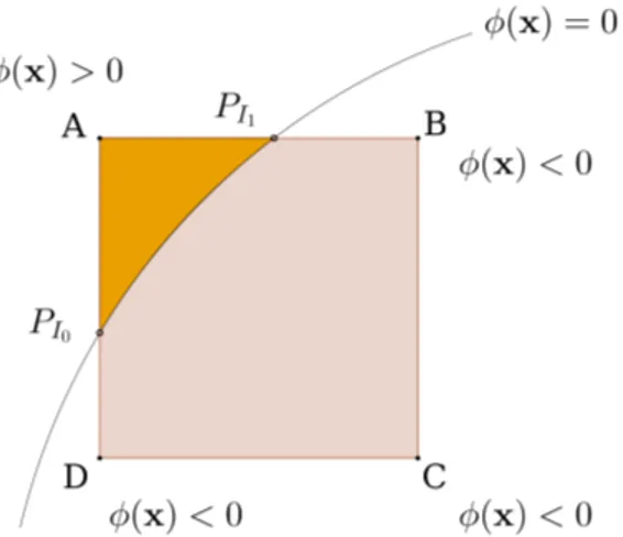
∀x ∈ Th:      φ (x) > 0 _{⇐⇒ x ∈ Ω}2 φ (x) = 0 _{⇐⇒ x ∈ Γ} φ (x) < 0 ⇐⇒ x ∈ Ω0. (2.37) For example, the unit circle geometry in 2D, used in this work, can be represented by the signed distance function:

φ (x) =�x2_{+ y}2_{− 1.} _(2.38)

The function is projected onto the computational mesh so that each node is marked with a level-set value. An example of implicit represen-tation of the surface on a cell is shown in Figure (2.3).

Figure 2.3. Example of a cell cut by the interface and the resulting level-set values on the nodes.

(27)

An example of the projection of the level-set function on a mesh is represented in Figure (2.4). The isocontour of zero values, representing φ (x) = 0, is obtained by interpolation and is shown as a white line.

Figure 2.4. The level-set function (2.38) projected onto a mesh, with the zero values represented by the isocontour in white.

Boundary representation

The first step for the interface approximation is to project the level-set function onto the triangulation and identify elements that are fully con-tained in Ω0, fully contained in Ω2or those which are cut by the interface

Γ, K ∈ Gh. To identify these elements, one has to analyze the projected

values of the level-set function on the nodes of the element. In order to facilitate the identification of elements, the following classification is proposed:

Nodes:

• Type 0 nodes: node P0= (x), φ (x) < 0

• Type 1 nodes: node P1= (x), φ (x) = 0

(28)

Cells:

It is convenient to evaluate the number of nodes of each type inside a cell as such: NP0, NP1 and NP2 for type 0, 1 and 2 nodes respectively. A diagram of element characterization is shown in Figure (2.5).

• Type 0 cell: a cell is considered to be "inside" if it is completely inside the subdomain Ω0 if it possesses all nodes of the type 0 or

type 1.

� K _{∈ Ω}0 if NP2 = 0and NP0+ NP1 = 4.

• Type 1 cell: a cell is classified as an "interface" cell if it has at least one node of type 0 and one node of type 2.

� K _{∈ G}h if NP1 ≥ 0 and 4 > NP0 > 0 and 4 > NP2 > 0. • Type 2 cell: a cell is classified as an "outside" cell if all its nodes

are of the type 1 or 2. � K ∈ Ω2 if NP0 = 0. Faces:

It is relevant to characterize only faces belonging to elements of Type 1 cell, i.e., K ∈ Gh. Faces are characterized as:

• Type 0 faces: faces F ∈ FG\ FS, i.e., F = K ∩ K�, where K ∈ Gh

and K�_{∈ Ω}₀_.

� if at least one node is of type P0 and the other is of type P0

or P1.

• Type 1 faces: faces intersected by Γ, i.e., F ∈ FS.

� if one node is of type P0 and the other is of type P2.

• Type 2 faces: faces F /∈ FG.

� if one node is a node of type P2 and the other is of type P1 or

P2.

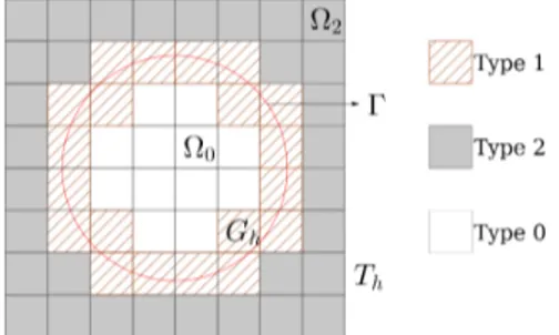
Figure 2.5. Diagram of a domain Thcut by an interface Γ given by the level-set

function φ = x2_{+ y}2

− 1 and the resulting classification of cells and domain characterization.

Intersection Detection

The next step of the boundary characterization is to find the points of intersection of Γ with the faces of cells K ∈ Gh. An intersected face

(29)

is characterized by having the level-set value on two consecutive nodes with diﬀerent signs (face of Type 1). One can compute the coordinates of the intersection points via a linear interpolation of the two values of the level-set on these nodes. In boundary problems where the domain of interest is only Ω0, a "new" cut-cell structure is created for elements

K ∈ Gh. For elements K ∈ Ω0, cell information is retrieved from the

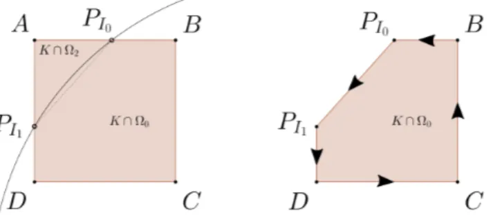
native deal.II framework for cell data. In Figure (2.6) an example of a cell intersected by the boundary is shown. Note that in the original cell there are 4 faces: AB,AD,DC and CB. In the second case, the cut-cell has 3 new faces: PI0B,PI0PI1 andPI1Dplus 2 original faces: DC and CB. The new cut face representing the local boundary of the cell, PI0PI1 , is marked as a boundary face, whereas other faces are internal faces. The described algorithm and structure of cell data does not lose generality for the case where the new cut cell has 4 or 3 faces.

Figure 2.6. Example of a cell intersected by the boundary and the resulting cut-cell, with nodes ordered counterclockwise.

In Algorithm (2.2) it is shown a simple sequence of steps used to detect intersection points and compute new relevant information about the cut cell. The process starts by looping over all cells from set Gh, then

identifying which faces are cut by the interface and which are completely inside Ω0or Ω1. New faces are created as described earlier and nodes are

reordered in an anti-clockwise manner, to facilitate further parametric representation and numerical integration.

This information is stored into a class type, in order to facilitate the retrieval of data in future computations. This class possesses the follow-ing relevant information about the cut-cell:

• Cell index • Centroid coordinates • Number of faces • Face information � Nodes’ coordinates � Normal vector � Face length

(30)

� Face index

� Face identification (boundary face/internal face).

Some properties of the new cut cell may be inherited from the native non-cut-cell from which it derives. For instance, normal vectors of faces that are not intersected by the boundary remain the same from the original cell. In these cases, the information is merely copied from the native cell container provided by deal.ii. When new data need to be computed, functions inside the class calculate and set these new parameters. This approach is also advantageous because it provides an easy and eﬃcient way to retrieve cells and faces through indices and to verify the type of faces, facilitating the integration of terms over the boundary.

Algorithm 2.2Intersection Detection for each K ∈ Gh

for each F ∈ K

if φ(X0)∗ φ(X1)≤ 0

Compute intersection point PIi i←i+1

if φ(X0) < 0

Create new face X0PIi else if φ(X1) < 0

Create new face X1PIi

Reorder nodes in anti-clockwise order Compute normal vector

Create new face PI0PI1

Reorder nodes in anti-clockwise order Compute normal vector

Store data about cut-cell

2.6.3 Integral Evaluation on Cut-Cells

The next step is to evaluate integrals defined on the domain Ω0 and in

the boundary Γ. These integrals can be, for example, of the type ˆ K ∇φi· ∇φjdx dy and ˆ K f φjdx dy (2.39)

from (2.16) on the area of cut-cells K ∩ Ω and ˆ

ΓN

gNφjdΓ (2.40)

(or similar) from eq. (2.17) on the boundary Γ, as explained in section (2.5.1).

(31)

The numerical integration procedure provided by deal.II evaluates in-tegrals over standard quadrilateral elements and faces only. By cutting arbitrarily an element, one can have as a result elements with 5, 4 or 3 faces, as shown in section (2.6). The integrals must be evaluated only on the part of the cut-cell inside the domain Ω. One possible alternative would be to split this element and create new quadrilaterals conforming to the boundary, a technique frequently used in the extended FEM [6, 50]. These new quadrilaterals would be part of a new "sub-triangulation" and one could take advantage of the native integration over quadrilaterals provided by deal.II. However, this process would require the generation of a new triangulation structure which may need additional vertices, becoming expensive and defeating the purpose of avoiding grid reinitial-ization. An alternative approach is to use Schwarz-Christoffel conformal mappings, as described by Natarajan, et al. [37, 38] in the X-FEM framework. This method is efficient for 2D problems but appears to be difficult to extend to three dimensional space.

The approach used in this work is based on the reduction of face inte-grals to boundary inteinte-grals through Green’s Divergence theorem. This method was described by Mirtich [35] and was eﬃciently applied to calcu-late solid mechanics properties such as moments and product of inertia in polyhedral bodies. The method was extended to the finite element framework by Massing, et al., [34] and successfully used to evaluate in-tegrals such as (2.39) in complex polygons and polyhedra.

First, the concept of multi-index and its notation are introduced, which are used throughout the text.

A multi-index α = (α0, α1,· · · , αdim−1)∈Ndim−10 is defined as a

dim-tuple of non-negative integers αi. Its order |α| is

|α| =

dim_�−1 i=0

αi. (2.41)

Based on this, the classical partial derivative can be written as Dαu = dim_�−1 0 � ∂ ∂xi �αi u. (2.42)

The method for evaluating integrals over cut-cells is outlined by the following steps:

1. Rewrite integrands on a monomial basis.

The terms to be integrated on cut-cells such as (2.39) can be interpo-lated onto a monomial basis. Let x = [x0,· · · , xdim−1] ∈ R2 be the

natural space for Cartesian coordinates. A polynomial f (x0, x1, ...)can

(32)

f (x) = c0(x)α0+· · · + cn(x)αn = n

�

i=0

ci(x)αi, (2.43)

where α is a multi-index dim-tuple and xα= xα0 0 · xα11· · · · x αdim−1 dim−1 = dim−1_� j=0 xαj j . (2.44)

2. Reduce integrals over surfaces (dim = 2) to line integrals.

The two-dimensional Divergence Theorem of Gauss reads [47]: Let R be a domain in the xy-plane with boundary curve C. If �F is a smooth vector field, ¨ R ∇ · �F dA = ˛ C � F _{· ˆ}n dS (2.45)

To employ this theorem, one must rewrite the polynomial integrand f (x, y) as the divergence of the vector field ∇ · �F . This can be done by taking the anti-derivative of the monomials in the following fashion:

xα =∇ · dim−1_� j=0 xα+ej dim(αj+ 1) , (2.46)

where ej is the j-th unit vector.

It is easy to see that for the two-dimensional case the relation becomes: (x, y)α=∇ · � xα0+1· yα1 2(α0+ 1) ,x α0· yα1+1 2(α1+ 1) � . (2.47)

Now the polynomial f (x, y) can be written as

f (x) =∇ · �F (2.48) where � F = n � i=0 ci dim_�−1 j=0 xαi+ej dim(αij+ 1) . (2.49)

Equation (2.45) applied to an integral such as (2.39) over a 2D cell becomes: ˆ K f (x, y) dx dy = n � i=0 ci dim−1_� j=0 ˛ C xαi+ej dim(αij+ 1)· ˆ n dS (2.50)

(33)

The closed curve integral can be approximated by the sum of line integrals along the faces of the element, that together form a closed convex polygon: ˆ K f (x, y) dx dy = n � i=0 ci dim−1_� j=0 nf aces_�−1 k=0 ˆ Fk∈K xαi+ej dim(αij + 1)· ˆ nFkdF, (2.51)

where Fkrefers to the kth- face of the cut-cell K and nf acesto its number

of faces.

3. Map face and evaluate line integrals.

The next step is to map and evaluate line integrals appearing in (2.51). To simplify the equations, the face integral will be represented as:

ˆ F∈K (x)αj+ei dim(αji+ 1) · ˆnF dF = ˆ F � G(x, y)_{· ˆ}n dF. (2.52) To evaluate the integral of eq. (2.52) it is advantageous to param-eterize the face F onto a 1D line. The coordinates of a point on the face F are represented as functions of independent parameters through geometrical mappings. The parameters usually lie in the unit interval.

F can be parameterized by the vector function �r(t), with t ∈ [0, 1], such that

�r(t) = (x (t) , y (t)) , (2.53) where �r (t) is an aﬃne transformation from Cartesian natural coordinates x, y_∈_R2 _{to parameter space t ∈ R. The diﬀerential becomes:}

dF =��r (t)�� dt, where��r (t)��_{� is equal to length of the face, L}

e.

The integral of (2.52) can finally be written as ˆ F � G(x, y)· ˆn dF = 1 ˆ 0 � G(x (t) , y (t))· ˆn Ledt, (2.54)

which can be readily integrated by the Gauss quadrature method as described in (2.5.1). As an alternative, Mirtich (1996) evaluated these integrals with the use of Bernstein’s polynomials, which do not require the evaluation of quadrature points beforehand.

(34)

3. Test Cases

The present chapter introduces numerical examples solved using the cut-cell finite element method. First, we solve the classical Poisson equation as described in section (2.1). Next, the Laplace-Beltrami problem is proposed, and finally, a reaction-diﬀusion case is introduced.

3.1 Poisson Problem

3.1.1 Problem setup

The model described by Poisson’s equation with pure Dirichlet bound-ary conditions imposed weakly by Nitsche’s approach was solved using the cut-cell method in a two-dimensional disk with radius r = 1. The boundary is represented by the level set function

φ (x, y) = �

(x− x0)2+ (y− y0)2− r.

Recalling (2.1) and setting the forcing function, f = 1, and Dirichlet value, gD = 0, the equation to be solved is:

−∆u = 1 in Ω u = 0 on Γ = ∂Ω, which has an analytic solution:

u (x) = 1− |x|

2

4 .

The values of γD and γ1 from equations (2.12) and (2.15) were set as

5.0 and 0.1, respectively. The domain Ω was embedded in a rectangular domain [−1.5, 1.5] × [−1.5, 1.5] partitioned into squares of equal size. For details about the finite element formulation, see section (2.3).

3.1.2 Convergence Analysis

Condition number of the stiﬀness matrix

The described finite element formulation yields a condition number of the stiﬀness matrix with similar upper bound as the one resulting from

(35)

the standard finite element method. More details about the analysis can be found in [17].

Let U be any vector such that U ∈ RN _{where N = dim V}

h, and denote

its corresponding finite element function in Vh by uh. The standard

Euclidean norm is defined by |U|N. Denote the mass matrix byM, which

is defined by the bilinear form (uh,vh), and the system matrix by A,

which is defined by the bilinear form Ah(uh,vh). The triangulation Th is

conforming to the domain ΩT. Therefore the following estimate hold:

µ1/2_min_�U�_N _{≤ �u}h�0,ΩT ≤ µ

1/2

max�U�N,

where µmin and µmax refer to the smallest and largest eigenvalues of

the mass matrix M. The condition number of the stiﬀness matrix A is represented by κ (A) and by definition is given by:

κ (A) =_�A��A−1�� , where �A� = sup U∈RN �AU�N �U�N .

The condition number of the system matrix arising from the finite element formulation using Nitsche’s method (2.13) satisfies the upper bound:

κ (A)_{≤ C h}−2 (3.1)

where C is a constant independent of how the boundary transverses the mesh. The proof and definition of C are given in [9].

Optimal error bounds

The finite element solution uh satisfies the following error estimates in

H1 _{and L} 2, respectively [9]: �u − uh�H1_(Ω)≤ C h �u�_H2_(Ω) �u − uh�L2(Ω)≤ C h 2 _�u� H2_(Ω).

3.2 Laplace-Beltrami Problem

3.2.1 The Laplace-Beltrami Model Problem

The pure diﬀusion equation on a closed surface Γ of co-dimension one is proposed as a model problem:

(36)

− ∆Γu = fon Γ, (3.2)

where ∆Γ denotes the Laplace-Beltrami operator, which will be defined

in the following sections. Since any constant function is a solution to this problem, one has to impose an additional constraint to obtain a unique solution. In this problem the mean value of u is chosen to vanish on the boundary, so that:

ˆ

Γ

u ds = 0. (3.3)

The first step to obtain a computable form of (3.2) is to define a suitable function space. The space of continuous Lagrange bilinear poly-nomials is used. The space VS is then introduced, with the enforcement

of constraint using a Lagrange multiplier method: VS = � v∈ H1(Γ)| ˆ Γ v ds = 0 � . (3.4)

To obtain the variational form, the same procedure outlined in section (2.1.1) is employed, as well as the notation regarding mesh characteris-tics. First, multiply the strong form (3.2) by a test function v ∈ VS and

integrate using Green’s formula. The weak formulation then reads: find u_{∈ V}S such that

a (u, v) = f (v) , _{∀v ∈ V}S (3.5)

where a (u, v) denotes the symmetric bilinear form on Γ and f (v), the linear functional form:

a (u, v) = (∇Γu,∇Γv)Γ (3.6)

f (v) = (f, v)_Γ (3.7)

3.2.2 Approximation of the Domain

Let p (x) be the closest point mapping on Γ to a point x ∈ Rdim _and

d (x)a signed distance function given by

d (x) =|p (x) − x| inRdim_\Ω _(3.8)

d (x) =_{− |p (x) − x| in Ω.} (3.9) The open tubular neighborhood of the boundary Γ is defined as:

(37)

U (Γ) =�x∈Rdim _:_{|d (x)| < δ}�_, _(3.10)

where δ is small enough so that for each x ∈ U (Γ) there is a uniquely determined p (x) ∈ Γ. See fig. (3.1) for a representation of the domains of interest. Let φ : Γ → R be any function defined on the hypersurface Γ. The smooth extension of φ to the neighborhood U is defined as:

�

φ (x) = φ_{◦ p (x) .} (3.11)

Note that �φ_|Γ = φ.

Let Ω1 be a domain in Rdim containing Ω ∪ U (Γ) and Th an uniform

triangulation of Ω in regular quadrilaterals K with mesh diameter h. A continuous piecewise linear approximation Γh of Γ is considered such

that Γh ⊂ U (Γ) and Γh∩ K is a subset of a hypersurface inRdim.

Figure 3.1. Representation of the described domains. U (Γ) is the green region where a unique closest point p (x) ∈ Γ is defined for each x ∈ U (Γ).

3.2.3 The Laplace-Beltrami Operator

The Laplace-Beltrami operator is a generalization of the Laplace oper-ator that operates on functions defined on surfaces in Euclidean space. Similarly to the Laplacian, the Laplace-Beltrami operator can be defined as the divergence of a gradient. In this section only a brief review of the operator is outlined, for more details refer to any book on diﬀerential geometry [45, 30].

For each x ∈ U (Γ), the projection of Rdim _{onto the tangent plane of}

(38)

PΓ= I− n ⊗ n, (3.12)

where I is the identity tensor and n, the normal vector. The tangential gradient of a function φ ∈ C¹ (U (Γ)) at x ∈ Γ is given by:

∇Γφ (x) = PΓ∇φ (x) , (3.13)

where ∇ is the usual gradient operator in Rdim_{. Finally, the}

Laplace-Beltrami operator for a C2_{(U (Γ))} _{function φ is defined as:}

∆Γφ (x) =∇Γ· ∇Γφ (x) . (3.14)

3.2.4 Finite Element Formulation

In order to discretize the formulation, the set of elements K associated with the boundary Γ is defined as follows, in the same fashion as in section (2.2): Gh= � K _{∈ T}h: K∩ Γh�= /O � , Ωh = � K∈Gh K. (3.15)

Let Vh,1 _{be the space of continuous piecewise linear functions defined}

on the triangulation Th. The function space Vhis defined as a continuous

piecewise linear function on Gh with average zero along the boundary:

Vh = � vh ∈ H1 : Vh,1|Ωh : ˆ Γ vhdΓ = 0 � . (3.16)

The standard Galerkin discretization of (3.5) reads: find uh ∈ Vh such

that

Ah(uh, vh) = L (vh) , ∀vh ∈ Vh, (3.17)

where the bilinear form is given by

Ah(uh, vh) = (uh, vh)Γh+ γSh jh(uh, vh) (3.18) and

L (vh) = (f, vh)Γh. (3.19) The stabilization term jh(uh, vh) is defined by

jh(uh, vh) =

�

F∈FS

(39)

where [∇u] denotes the jump of u over the face F . For definitions of jump term and set FS, see (2.2).

3.2.5 Problem Setup

The pure diﬀusion Laplace-Beltrami problem was solved using the cut-cell method in a circular domain with radius r = 1. The right hand side function f was chosen to be:

f (x, y) = 9 sin (3 arctan (x_/_y₎₎ (3.21)

as in [29] so that the analytical solution is

u (x, y) = sin (3 arctan (x_/_y_{)) .} (3.22)

The boundary domain Γ is defined by a circle of radius r = 1, and is obtained by the level-set function

φ (x, y) = �

(x− x0)2+ (y− y0)2− r.

The domain is embedded in a rectangular triangulation Th = [−1.5, 1.5] × [−1.5, 1.5]

comprised of squares of equal size. The triangulation is divided into sub-domains Ω0, Gh and Ω2 as described in section (2.6.2). Cells from

domain Ω0 and Ω2 were excluded from the computation. The

stabiliza-tion parameter γS was set to 0.01.

Condition Number of the Stiﬀness Matrix

Similarly to the Poisson model problem, the condition number of the stiﬀness matrix κ (A) is proportional to h−2 _{and the following estimate}

holds independently of the boundary intersection:

κ (A)_{≤ C h}−2. (3.23)

Optimal error bounds

The error estimates in H1 _{and L}

2 norms are, respectively:

�u − uh�H1_(Γ)≤ C h �u�_H1_(Γ) (3.24) �u − uh�_L₂_(Γ)≤ C h2 �u�_L₂_(Γ). (3.25)

(40)

3.3 Reaction Diﬀusion Problem

3.3.1 The Reaction Diﬀusion Problem

The proposed system is composed of a circular domain where a species A diﬀuses on the bulk domain and reacts in a patch of the membrane, identified by Γ1⊂ Γ, yielding a component B. The reaction mechanism

is given by a simple first-order reaction with reaction rate constant k:

A_{→ B}k (3.26)

The component B is membrane-bound and it is allowed to diﬀuse freely on it. The component A can be present both in bulk and membrane domains. The rates of reaction are expressed as:

rA=−rB=−k uA. (3.27)

The reaction occurs only on part of the boundary, hence the reaction term is defined by a Kronecker delta function δ (x). We choose Neumann no-flux boundary conditions on all the boundary, meaning that it is an enclosed domain with no exchange with the exterior. The final coupled system reads: ∂uA ∂t − ∇ · DA∇uA+ δ (x) k uA= 0, in Ω (3.28) n_·∇uA= 0, on Γ (3.29) ∂uB ∂t − ∇Γ · DB∇ΓuB− δ (x) k uA= 0, on Γ. (3.30) The weak form is obtained by the same procedure previously outlined. For the bulk equation: multiply (3.28) by a test function vA ∈ H¹ (Ω),

integrate using Green’s theorem: �

∂uA

∂t , vA �

+ a (uA, vA) +�δ (x) k uA, vA� − L (vA) = 0, (3.31)

where L (vA) =�vA, gN�. For the surface equation, multiply (3.29) by a

test function vB ∈ H1(Γ), integrate:

� ∂uB

∂t , vB �

(41)

3.3.2 Finite Element Formulation

The space discretization of the PDE system is based on the finite element formulation from the previous test cases. We use the space of bilinear Lagrange elements defined in eq. (2.8):

V_Ah=�v : v∈ C0(Ω) , v|K ∈ Q1(K) , ∀K ∈ Th

�

and in eq. (3.4) (except we do not enforce the constraint on the bound-ary):

V_Bh ⊂ V = H1(Γ) . The discretization then becomes:

� ∂uh A ∂t , v h A � + Ah � uh_A, v_Ah�+�δ (x) k uh_A, v_Ah�− L�vh_A�= 0 (3.33) � ∂uh_B ∂t , v h B � + Ah � uh_B, vh_B�−�δ (Γ) k uh_A, v_Bh�= 0. (3.34) Time discretization was performed using the Crank-Nicolson method [14], which is stable for the PDE system. The solution u, where u can be uA or uB, is replaced by the following approximation:

u (x, t) = (1_{− θ) u}n−1+ θ un (3.35) where n is the time step and θ is a parameter that tune the approxi-mation. For example, if θ = 0, the formulation reduces to the explicit Euler method. If θ = 1, it reduces to the pure implicit backward Euler method. In the Crank-Nicolson method, we choose θ = 0.5 and the time stepping is implicit and unconditionally stable. The derivative with time is approximated by:

∂u (x, t)

∂t =

un_{− u}n−1

∆t (3.36)

To obtain the final linear system, the eqs. (3.35) - (3.36) are replaced into (3.33). After, the solution uh _{is replaced by u}h ₌�

j

Ujφj and the

test function by vh _{= φ}

i as usual.

The stabilized Nitsche’s method is used to enforce Neumann boundary condition in (3.33), using the formulation (2.13) for the bilinear term Ah

�

v_Ah, uh_A�and the formulation (2.12) for the term L�vh_A�. The final equation to be solved is:

(42)

� MΩ+ θ ∆t �AΩ+ k MΓR �� U_An =�MΩ− (1 − θ) ∆t � k M_ΓR+ AΩ �� U_An−1, (3.37) where the stiﬀness matrix AΩ is

(AΩ)ij = (∇φi,∇φj)_Ω+�γNh nΓ· ∇φi, nΓ· ∇φj�_Γ

+γ1h jh(φi, φj)_FG. (3.38) The mass matrix MΩ is also stabilized by adding stabilization terms:

(MΩ)_ij = (φi, φj)_Ω+ γMh2jh(φi, φj)_F_G. (3.39)

The mass matrix MR

Γ is the mass matrix arising from the reaction

term, which occurs only on part of the domain, defined by the function δ (x). The matrix is also stabilized:

�

M_ΓR�_ij = (δ (x) φi, φj)_Ω+ γMh2jh(φi, φj)_F_S. (3.40)

The linear system used to solve eq. (3.34) is obtained by taking the same steps. The final equation is:

[MΓ+ θ ∆t AΓ] UBn

= [MΓ− (1 − θ) ∆t AΓ] U_Bn−1+ k CΓ∆t. (3.41)

Here, the stabilized form of the bilinear term (3.18) was used to define Ah

�

uh_B, v_Bh�, so that the stiﬀness matrix AΓ is

(AΓ)_ij =�∇Γφi,∇Γφj� + γSh jh(φi, φj)_F_S. (3.42)

The mass matrix MΓ is also stabilized and becomes:

(MΓ)ij =�φi, φj�_Γ+ γMh2jh(φi, φj)_F_S. (3.43)

The vector Cn

Γ is obtained from the integration of the reaction term

and depends on the concentration of un

A. It is given by:

(C_Γn)_ij =�δ (Γ) uA, φi�Γ, (3.44)

where uA is obtained by eq. (3.35) from the already computed unA and

un_A−1. The resulting linear systems to be solved at each time step are eqs. (3.37) and (3.41).

(43)

3.3.3 Problem Setup

The set of PDE’s was solved using the cut-cell method in a circular domain of radius r = 1, so that the boundary Γ is represented by the level-set function

φ (x, y) = �

(x− x0)2+ (y− y0)2− r.

The boundary Γ was split into two subdomains: Γ1, represented by

the third quadrant of the circle, given by

Γ1 ={(x, y) ∈ Γ : x < 0, y < 0} (3.45)

and Γ2, represented by the remaining quadrants:

Γ2 ={(x, y) ∈ Γ \ Γ1} . (3.46)

The delta function δ (x) is then defined as: δ (x) =

�

1 if Γ = Γ1

0 if Γ = Γ2

The reaction rate constant was set to k = 100. The diﬀusion co-eﬃcients are homogeneous over all the domain and were both set to DA = DB = 0.1. As initial condition, a concentration of uA = 400 was

set on a square [−0.25, 0.25] × [−0.25, 0.25] and equal to zero elsewhere. A diagram of the initial conditions and geometry is shown in Figure (3.2). Concentration of B was set to zero everywhere.

The solution was solved for a total time of tf = 3.0s, with a time

step equal to ∆t = 0.004 s. The parameters were selected as follows: γ1 = 0.1;γS = 0.01; γM = 0.1; γD = 5 and γN = 1.

(44)

3.3.4 Mass Conservation

Since there are no generation terms nor flux across the boundary, the total variation of mass in the domain should approximate zero. In order to ensure that the mass is conserved throughout the time interval, we compute the total mass Mti in the domain at each time step ti using the following equation: Mti = nK � Ki∈Ω ˆ Ki uti AdΩ + n_Gh � Γ_Ki∈Gh ˆ Γ_Ki uti BdΓ (3.47)

and evaluate the variation of Mtirelative to the initial mass present in the domain with

∆Mti = � � � � Mti− Mt0 Mt0 � � � � × 100%. (3.48)

(45)

4. Results

4.1 Poisson’s Problem

4.1.1 Solution

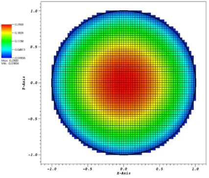
The solution for the problem is shown in Figure (4.1) below. The bound-ary is represented by the thick black line. After removing the elements completely outside Ω, the mesh contains 13104 elements, each of diam-eter 0.0220971.

Figure 4.1. Solution for the Poisson problem with B.C. imposed weakly with Nitsche’s method.

(46)

The numerical solution was compared with the exact solution and the L2(Ω)and H1(Ω)norms were evaluated, as shown in Figure (4.2).

Figure 4.2. Convergence analysis in H1 _{(orange) and L}

2 (blue) norms. The

dashed lines are proportional h (orange) and h2_(blue).

4.1.3 Matrix conditioning analysis

This section shows the eﬀects on the condition number of the stiﬀness matrix with respect to the mesh size and the stabilization parameter.

First the relation κ (A) ≤ C h−2_{, detailed in (3.1.2) was analyzed. In}

Fig. (4.3) the condition number of the stiﬀness matrix is plotted versus the inverse of the cell diameter.

Figure 4.3. Condition number as a function of the inverse of the cell diameter. The dashed line is proportional to h−2_.

(47)

Next, the eﬀect of stabilization parameter γ1is evaluated, for the most

refined case as shown in section (4.1.1).

Figure 4.4. Condition number as a function of γ1.

In order to evaluate the dependence of the solution with the stabiliza-tion parameter, the L2 norm was plot versus γ1 and the results can be

seen in Figure (4.5).

(48)

4.2 Laplace-Beltrami Problem

4.2.1 Solution

The equation was solved on cells K ∈ Gh and the solution is shown on

Γh, as can be seen in (4.6). The cell diameter is h = 0.022 and the mesh

contains 3332 cells, with 504 degrees of freedom.

Figure 4.6. Solution on a boundary defined by the level set function.

The H1 _{and L}

2 errors were evaluated based on the solution obtained on

(49)

Figure 4.7. Convergence analysis in H1 _{(orange) and L}

2 (blue) norms. The

dashed lines are proportional h (orange) and h2_(blue).

4.2.3 Matrix conditioning analysis

The mesh dependence of the condition number was evaluated and the results can be seen in Figure (4.8).

Figure 4.8. Dependence of condition number with the element size. The dashed line is proportional to h−2_.

4.3 Reaction-Diﬀusion Problem

4.3.1 Solution

The concentration profile of component A is shown in Figure (4.9), with the correspondent time associated. The mesh contains 13104 elements, each of size 0.0220971.

(50)

Figure 4.9. Time snaps of concentration of component A. The boundary is represented by the level set function in white.

Figure 4.10. Concentration profile of component B on the boundary Γh.

4.3.2 Mass conservation

Mass conservation was calculated using (3.47) and the results of total mass variation are depicted in Figure (4.11).

(51)

(52)

5. Discussion

5.1 Poisson’s Problem

The solution for the Poisson’s problem is shown in section (4.1). It is important to note how the final solution contains nodes that are in fact outside the domain of the problem. These nodes are of "type 2" as represented by node A on section (2.3). These nodes were kept in the solution representation to illustrate how they play a role in the solution process, but do not represent the final solution of the problem. More-over, the solution clearly follows the well known expected pattern of the homogeneous Poisson’s equation on a disk.

The convergence analysis shows optimal convergence of second order in L2and first order in H1as expected from the finite element formulation.

The integration over small parts of elements adversely aﬀects the con-dition of the stiﬀness matrix. This is overcome by adding stabilization terms (2.15) in the finite element formulation, which can be tuned by the parameter γ1. In Fig. (4.4), the plot of the condition number as a

function of the stabilization parameter γ1 is shown. It was observed that

very small values of γ1 lead to bad conditioning (γ1 = 0.015), whereas

the simulation with γ1= 0.05 resulted in the smallest condition number

observed. After this value, the condition number increases steadily with the increase of γ1. Burman and Hansbo [9] report a very resembling

pattern for a similar problem, where they found the condition number to be optimal for γ1= 0.01.

In addition, the L2 error was evaluated for diﬀerent values of the

stabilization parameter. The error has a peak for γ1 = 0.015 and the

lowest value when γ1 = 0.1, and grows linearly afterwards from γ1 = 0.1

to 1. This relationship shows a close resemblance with the dependence of the condition number on γ1 (Fig. (4.4)). Based on these results, it

is suggested that in order to achieve a low condition number and error, one should set the stabilization parameter to γ1 = 0.05or 0.1.

The dependence of the condition number on the mesh size was evalu-ated, and confirmed to be of second order as estimated.