Disocclusion Inpainting using Generative Adversarial Networks

(1)

Master's thesis

Two years

Datateknik

Computer Engineering

Disocclusion Inpainting using Generative Adversarial Networks

(2)

MID SWEDEN UNIVERSITY

Department of Information Systems and Technologies (IST) Examiner: Mårten Sjöström, marten.sjostrom@miun.se Supervisor: Elijs Dima elijs.dima@miun.se

Author: Nadeem Aftab naaf1001@student.miun.se nadeem408@gmail.com

Degree programme: International Master’s Programme in Computer Engineering 120 credits

Main field of study: Computer Engineering Semester, year: HT, 19

(3)

Abstract

The old methods used for images inpainting of the Depth Image Based Rendering (DIBR) process are inefficient in producing high-quality virtual views from captured data. From the viewpoint of the original image, the generated data’s structure seems less distorted in the virtual view obtained by translation but when then the virtual view involves rotation, gaps and missing spaces become visible in the DIBR generated data. The typical approaches for filling the disocclusion tend to be slow, inefficient, and inaccurate. In this project, a modern technique Generative Adversarial Network (GAN) is used to fill the disocclusion. GAN consists of two or more neural networks that compete against each other and get trained. This study result shows that GAN can inpaint the disocclusion with a consistency of the structure. Additionally, another method (Filling) is used to enhance the quality of GAN and DIBR images. The statistical evaluation of results shows that GAN and filling method enhance the quality of DIBR images.

Keywords: depth image-based rendering (DIBR), generative adversarial network (GAN), neural network, disocclusion

(4)

Acknowledgments

First and foremost, I would like to thank my friends who helped me dur-ing this project. Secondly, I am very grateful to Professor Mårten Sjöström who gave me this opportunity. I would like to especially thank my super-visor Elijs Dima who was very helpful throughout my thesis work and guided me through the whole project.

(5)

List of Figures

Figure 1.1: DIBR generated image from the MSR 3D video dataset [8]. . 11

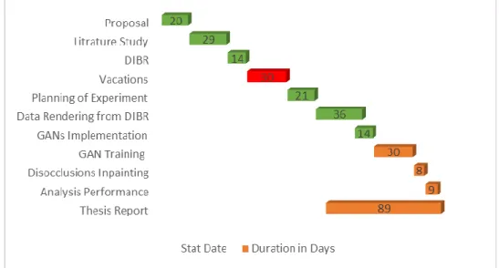
Figure 1.2: Thesis planning outline. ... 12

Figure 2.1: ML is an application of AI [15] ... 16

Figure 2.2: Basic neural networks ... 17

Figure 2.3: Multilayer perceptron [18] ... 17

Figure 2.4: Multilayer perceptron with activation [19] ... 18

Figure 2.5: NN cycle [20] ... 19

Figure 2.6: Basic NN example with weight and biases [21] ... 20

Figure 2.7: NN example with initial weight and biases [21] ... 20

Figure 2.8: CNN architecture detail [23] ... 22

Figure 2.9: Deep learning CNN for image classification [22] ... 23

Figure 2.10: Overall concept of GAN [25] ... 24

Figure 2.11: GAN architecture ... 25

Figure 2.12: Discriminator training ... 26

Figure 2.13: Generator training ... 26

Figure 2.14: Camera model: (a) Projections illustration; (b) Geometric relations [13] ... 27

Figure 2.15: Virtual camera view from original cameras [33] ... 30

Figure 2.16: DIBR system block diagram [37] ... 31

Figure 3.1: Ground truth and depth map of an image of Cam 1 ... 33

Figure 3.2: Ground truth and depth map of an image of Cam 7 ... 33

Figure 3.3: Proposed GAN architecture ... 34

Figure 4.1: Generator parameters summary ... 40

Figure 4.2: Discriminator model ... 41

Figure 4.3: Discriminator parameters summary ... 42

Figure 4.4: GAN training ... 43

Figure 4.5: Before combining both images ... 44

Figure 4.6: Replacing holes (missing pixel) with GAN pixel ... 44

Figure 4.7: Used libraries for time PSNR/SSIM computation ... 45

Figure 4.8: PSNR computation ... 46

Figure 4.9: SSIM computation ... 46

Figure 4.10: T-test for PSNR ... 46

Figure 4.11: T-test for SSIM ... 46

Figure 5.1: Virtual view from camera 1 to virtual cameras... 47

Figure 5.2: Output after 1st_{iteration out of 130 ... 48}

Figure 5.3: Output after 60th_{iteration out of 130 ... 48}

(8)

Figure 5.6: GAN image ... 51 Figure 5.7: Filled image and ground truth ... 52 Figure 5.8: Mean PSNR and 95% confidence intervals comparison ... 54 Figure 5.9: Mean PSNR and 95% confidence intervals of DIBR, GAN, and filled methods ... 54 Figure 5.10: SSIM Mean and confidence intervals comparison of DIBR, GAN, and filled methods ... 55 Figure 5.11: SSIM comparison of the mean of DIBR, GAN, and filled methods ... 56

(9)

Terminology

Abbreviations

ML Machine Learning

AI Artificial Intelligence

NN Neural Network

ANN Artificial Neural Network

CNN Convolutional Neural Network

DIBR Depth Image-Based Rendering

GAN Generative Adversarial Network

ReLU Rectified Linear Unit

PSNR Peak Signal to Noise Ratio SSIM Structural Similarity Index

SGD Stochastic Gradient Descent

MLP Multilayer Perceptron

Mathematical notation

𝐺(𝑧) Generator generated output

𝐷(𝑥) Input for Discriminator of real data

𝐷(𝐺(𝑧)) Input for Discriminator of Generator’s output 𝐷(𝑥, 𝐺(𝑧)) Input for Discriminator of both real and fake data

(10)

1 Introduction

Generative Adversarial Networks (GANs) [1] have become very popular from the last five years and GANs become widely popular because of their application versatility and outstanding results for generating data. They have been used in many different types of applications like text, im-age, and video generation[2]. Depth Image Based Rendering (DIBR) [3] is a processing technique that generates virtual data using a depth map, be-cause of this process disocclusion occurs in generated data. Inaccuracies between texture image and depth map cause disocclusion[3]. GAN might also be beneficial to inpaint disocclusion generated because of DIBR.

1.1 Background and problem motivation

Generative Adversarial Networks (GANs) have been widely used re-cently because of their versatility for applications and competitive results in generating data. GANs are a type of machine learning algorithm, which consists of two neural networks, working against each other to generate authentic data (such as realistic images, faces, photo-graphs, visual or audio data content)[2]. The process of generating data through neural networks is often called hallucinating [4] for example GAN is hallucinating part of an image. GANs have been used for image and video corrections and processing applications[2].

Depth Image Based Rendering (DIBR) is a technique to render virtual views from real view. The view geometry information is given by an ad-ditional depth stream that stores for each pixel its distance to the camera. This technique allows the use of it for many applications including 2D-3D conversion. Depth Image Based Rendering (DIBR) is an important method for virtual synthesis but it always creates holes or can be de-scribed as missing spaces(occlusions) in the virtual view. The disocclu-sion problem occurs due to the fact the original view only captured from a single view which can lead to missing information in the generated vir-tual view [5]. DIBR always results in hole problems where depth and color values are not known. Holes mostly occur in the background of the image because the background is prone to occlusion by the foreground of the image[6]. Several methods can be used to fill the missing spaces(disocclusion), however previous hole-filling methods create other problems like cracks and edge-ghosting[7]. Generative Adversarial Net-works (GANs) can be used to overcome this problem.

(11)

1.2 Problem Description

Generating a three-dimensional (3D) structure from a two-dimensional image can create holes in the generated view. From the regular original two-dimensional image, a 3D structure seems normal, but when the struc-ture is rotated, gaps and missing spaces become visible, for all the sur-faces and spaces that were occluded or otherwise hidden in the original image. The old approaches for filling in disocclusion tend to be slow, in-efficient, and inaccurate. Modern solutions specially GANs can be better suitable for filling the missing spaces when they are trained. In particular, there is an opportunity to combine the GAN disocclusion inpainting with the generation of new viewpoints from a set of existing Multiview depth views. Multiview plus depths formate use view synthesis to generate in-termediate views from existing adjacent views. The below image is ren-dered from the MSR 3D video dataset(breakdancing) [8] through the DIBR process. The yellow color in the image indicates missing or un-known pixels.

Figure 1.1: DIBR generated image from the MSR 3D video dataset [8].

1.3 Tools, Requirements

MSR 3D video dataset(breakdancing) [8] is used for the Depth Image Based Rendering (DIBR) process in framework Python /Keras [9] using

(12)

Anaconda [10] to produce virtual data. GANs model deployed and train in Google Colaboratory.

1.4 Milestones

Milestone 1. Literature study: Initially reading about basics Machine

Learning (ML), Deep learning architectures learning, convolutional neural networks, and Generative Adversarial Networks (GANs).

Milestone 2. Literature study on Depth Image Based Rendering (DIBR):

Reading basic of two camera geometry, to know how to render virtual views from a 2D image and depth information.

Milestone 3. Data rendering with DIBR: To render dataset from MSR 3D

video dataset(breakdancing) code of Python.

Milestone 4. GAN training: Training of GAN on DIBR generated data,

experiment to inpaint the disocclusion of DIBR generated images through GAN.

Milestone 5. Disocclusion Inpainting: Inpaint disocclusion in DIBR

generated images through GAN.

Milestone 6. Performance Analysis: Analysing the results acquired from

the experiment.

Milestone 7. Thesis Report: write an analysis of the results, thesis

write-up. (Duration 160 hours).

Figure 1.2: Thesis planning outline.

1.5 Overall Aim

The overall aim of the project is inpainting of disocclusion generated from Depth Image Based Rendering (DIBR). To fulfill this purpose Generative

(13)

Adversarial Networks (GANs) methodology is adopted and results of this would determine if GANs help to inpaint occlusion occurs during Depth Image Based Rendering (DIBR). The output of this work can help to determine if this method is good or not to fill in disocclusion.

1.6 Goals

The below goals are set to achieve the basis of knowledge. The concrete goals are:

1. Generation of virtual data based on the DIBR process from the MSR 3D video dataset (breakdancing) [8] for all cameras.

2. Implementation and training of the GAN model.

3. Inpainting disocclusion through the GAN model of DIBR gener-ated data.

4. Analysis of results using Peak Signal to Noise Ratio (PSNR) [11] and Structural Similarity Index [12] methods.

1.7 Scope

The focus of this study to implement GANs architecture on the DIBR’s generated dataset to inpaint disocclusion occurs during Depth Image Based Rendering (DIBR) process. For data rendering, the DIBR process shall be implemented in Python as well as GAN’s model also imple-mented and train in Python, Keras. External sources such as Google Drive and Google Colaboratory shall be used to execute this model. Any parison with other networks like neural networks or any inpainting com-parison such as in a paper “Free View Rendering for 3D Video, Edge-Aided Rendering, and Depth-Based Image Inpainting” [13] would not be conducted. The personal computer has been used only for DIBR and for GAN model architecture but the GAN model executes in Google Cola-boratory because of memory constraints and limitation of resources.

1.8 Outline

The next section of this report describes the background of Machine Learning, Neural Networks, Generative Adversarial Networks, and DIBR. Section 3 describes the methodologies adopted to achieve the de-sired results. In section 4, the implementation of adopted methodologies is described. Section 5 shows the results of a successful implementation. In section 6, the conclusion of the project and achieved goals are dis-cussed.

(14)

1.9 Contribution

I am responsible for the planning of this project and with the implemen-tation of DIBR to generate virtual data and implement the GAN to get required results and assessment of obtained results plus writing the re-port of this project under the supervision of Elijs Dima and examiner Prof. Mårten Sjöström.

(15)

2 Theory

To understand Generative Adversarial Networks, one must have to un-derstand the basics of Machine Learning (ML), Neural Networks (NN), Convolutional Neural Networks (CNN), Generative Adversarial Net-works (GANs). Depth Image Based Rendering (DIBR), knowledge is also required to complete this project. In the coming sections, all these con-cepts are described one by one.

2.1 Machine Learning

Machine Learning (ML) can be described as the sub-field of Artificial In-telligence (AI) that uses data to teach a machine how to perform a task. The simplest scenario can be using a person’s face image as an input to the algorithm so that the machine/program can learn to recognize the same person in the image[2].

Donald Michie described that it would be impactful if machines could learn from experience to improve efficiency by learning from the program during execution. A simple but effective rote-learning facility can be pro-vided within the framework of a suitable programming language [14]. Now computers can learn from their experience and improve their effi-ciency, it’s called “Machine learning”. It is part of Artificial Intelligence (AI) that gives power to a system to learn and improve from their experi-ence. Its focus on the development of machine which can access data and learn from that data. The process of learning starts from the observation, data, or examples to check patterns in data to make decisions for the fu-ture. The main purpose of machine learning is to allow the system to do this whole process without any human interaction or help. There are two methods for machine learning which are supervised and unsupervised learning. Supervised learning can apply as what has been learned in the past and data is labeled and classified. This learning can apply to new data for using labeled to predict future events. An Unsupervised machine learning method or algorithm is when the data used to train is neither labeled nor classified. The purpose is to find hidden structure from this unlabeled data.

Below figure 2.1 is from Deep Leaning by Goodfellow [15] which shows that representation learning which is part of machine learning and ma-chine learning is a subpart of artificial intelligence.

(16)

Figure 2.1: ML is an application of AI [15]

Machine learning consists of three phases which are preparation, execu-tion, and evaluation. The first step preparation begins which gathers data for training and then prepares for a suitable model. The execution phase deals with the training of the system on a given model on training data to predict the outputs and update new features(weights) and intercepts(bi-ases). In the evaluation phase check generated results with evaluation data and if results are not accurate to add more iteration like the previous step to get more accurate results.

2.2 Neural Networks

Artificial Neural Networks (ANN) or Neural Networks (NN) consist of the multiple numbers of processing units that communicate by sending a large number of signals to each other over a large number of connections [16]. Neural Networks (NN) is a process to create a computer application that learns from data. A collection of connected layers does some specific task called neural at each layer and which communicate with other layers. Then assign a task to network and ask to solve the problem, it attempts to do, again and again, each time strengthen its connection that leads to suc-cess or failure. According to Gurney, Kevin neural networks are simple processing units that are interconnected and network functionality de-pends on the neuron. The network’s processing ability based on connec-tion strengths, its weight, and learning method from the training set[17].

(17)

2.2.1 Neural network architecture

Neural network architecture consists of different layers, below in figure 2.2 is the basic architecture of the neural network, on the most left its input layer and neuron of this layer is called input neurons. The rightmost layer is called the output layer, and neurons of this layer are called output neu-rons, in this architecture, it consists of only one neuron. The middle layer of this network is called the hidden layers and the neuron of this layer is neither called input or output. In this network, it consists of only one layer but different networks can have multiple network layers [18].

Figure 2.2: Basic neural networks

The following network figure 2.3 has two hidden layers and the network consists of four layers. Sometimes people called this architecture as mul-tilayer perceptron or MLPs use sigmoid activation function. The purpose of the activation function is to introduce non-linearity in networks.

(18)

2.2.2 Neural network training

Suppose a network consists of different inputs from

𝑥

₁

, 𝑥

_2,

. . , 𝑥

_𝑚 and weights

𝑤

₁

, 𝑤

_2,

. . , 𝑤

_𝑚 attached to every input as shown in figure 2.4. These weights are real numbers which are expressing the importance of respective input to output. The output of the neuron 0 or 1 determined by whether the sum of the weights is less than or greater than a specific threshold [18].

Figure 2.4: Multilayer perceptron with activation [19]

Most ANNs follow the “learning rule” get input from a random weight which gets more accurate over time. Biases and activation function ap-plied to the network and then calculate error and delta through backprop-agation with some adjustment to weight and biases. When weights and biases become accurate on any given inputs it produces pretty good re-sults from the system. figure 2.5 explains step by step architecture of neu-ral networks. There are many methods involve like Feed Forward, loss function Backpropagation.

(19)

Figure 2.5: NN cycle [20]

Neural Networks used many different rules for learning, one of the most common is the delta rule. This rule is mostly used by the most common class of ANNs called “Backpropagational Neural Networks” (BPNN). It is an abbreviation for the backward propagation of errors. Backpropaga-tion is used to calculate error and delta and adjust all the weights and biases of the previous layer until conditions are fulfilled or iterations are finished.

Hidden layers used sigmoidal activation function which helps to polarize and stabilize. The learning rate calculates how much any specific iteration affects the weights and biases and then Momentum calculates how much past iteration outcome affects weights and biases. We can calculate the change in a given bias by below formula

(𝐶ℎ𝑎𝑛𝑔𝑒) = (𝑙𝑒𝑎𝑟𝑛𝑖𝑛𝑔 𝑟𝑎𝑡𝑒 ∗ 𝑑𝑒𝑙𝑡𝑎 ∗ 𝑣𝑎𝑙𝑢𝑒) + (𝑚𝑜𝑚𝑒𝑛𝑡𝑢𝑚 ∗ 𝑝𝑎𝑠𝑡 𝑐ℎ𝑎𝑛𝑔𝑒)

(2.1)

Let’s take another example where the neural network takes two inputs

𝑖

₁and

𝑖

₂ and this network has 2 hidden layers and two output layers. The hidden and output layer includes biases too with weights. The basic structure looks like in figure 2.6.

(20)

Figure 2.6: Basic NN example with weight and biases [21]

To start the training of this network lets add some initial random weights and biases that are attached to the network as shown below.

(21)

The purpose of backpropagation is to update the weights so that the neu-ral network can learn to correctly and predict the output from a given input. From the feedforward, the net at each neuron is calculated by the dot product between its associated weights and the output activations from the previous layer. The output of the previous layer neurons is then calculated by the applying activation function and the process repeat it-self for all the neuron in all layers, Mathematical formula is below [21].

𝑛𝑒𝑡

_ℎ1

= 𝑤

₁

∗ 𝑖

₁

+ 𝑤

₂

∗ 𝑖

₂

+ 𝑏

₁

∗ 1

(2.2)

For calculating ℎ1total net input

𝑛𝑒𝑡𝑜1 = 0.4 ∗ 0.593269992 + 0.45 ∗ 0.596884378 + 0.6 ∗ 1 = 1.105905967

(2.3)

With the squash implementation of logistic function to get output for ℎ1

𝑜𝑢𝑡

_ℎ1

=

1

1+𝑒−𝑛𝑒𝑡ℎ1

=

1

1+𝑒−0.3775

= 0.593269992

(2.4)

The repetition of the process can get the values of others too. To calculate the error for each output neuron by using the squared error function and sum them to get the total error.

𝐸

_{𝑡𝑜𝑡𝑎𝑙}

= ∑

1

2

(𝑡𝑎𝑟𝑔𝑒𝑡 − 𝑜𝑢𝑡𝑝𝑢𝑡)

2

_(2.5)

To get the total error, sum the error of all output neuron’s error as below

𝐸

_{𝑡𝑜𝑡𝑎𝑙}

= 𝐸

_𝑜1

+ 𝐸

_𝑜2

(2.6)

Now goal with backpropagation is to update all the weights in the net-work so netnet-work output could come closer to the target output. Therefor network error could be minimizing for each neuron as well for the whole network. For example, in the network

𝑤

₅, after applying the chain rule the total error change would be [18].

𝜕𝐸_{𝑡𝑜𝑡𝑎𝑙} 𝜕𝑤₅

=

𝜕𝐸_{𝑡𝑜𝑡𝑎𝑙} 𝜕𝑜𝑢𝑡_𝑜1

∗

𝜕𝑜𝑢𝑡_𝑜1 𝜕𝑛𝑒𝑡_𝑜1

∗

𝜕𝑛𝑒𝑡_𝑜1 𝜕𝑤₅

(2.7)

By following this backward pass values for remaining neurons can calcu-late.

(22)

2.3 Convolutional Neural Networks

To learn about the hundreds of hundreds of objects from millions of im-ages or data, it needs a model with a large learning capacity. The com-plexity of object recognition makes it a difficult task that means this prob-lem cannot be specified for all types of data set, so our model should have some prior knowledge to suitable for all types of datasets. As compared to traditional feedforward neural networks with the same size, the con-volutional neural network has fewer connections and parameters so they are easier to train [22].

“To learn about thousands of objects from millions of images, need such model with large learning capacity” [23]. The convolutional neural net-work is the most popular artificial neural netnet-work which is used for im-age analysis”. A Convolutional Neural Network (ConvNet/CNN) is a Deep Learning algorithm that can take in an input image, assign im-portance (learnable weights and biases) to various aspects/objects in the image, and be able to differentiate one from the other” [23]. Image analy-sis is not the only case to use convolutional neural networks, they can be used for data analysis and classification problems as well. More generally we can say that artificial neural networks have some type of specializa-tion for picking out or detect patterns. Pattern detecspecializa-tion makes convolu-tional neural networks useful for image analysis.

Figure 2.8: CNN architecture detail [23]

The thing which makes convolutional neural networks better from others is hidden layers that receive input and transform input in some way to produce better output for the next layer of the convolutional network. This transformation is a convolutional operation. Each layer has several filters that detect patterns. The pattern can be edge detection, circle or corner and the next layer can detect images like an eye, finger, etc. and the final layer can detect the whole image.

(23)

Top deep convolutional neural networks architecture typically organized into an alternative convolutional layer and max-pooling neural networks layer followed by some dense and fully connected layers as Krizhevsky [22] described. The input 3D (RGB) image representation is the input layer and then transforms into a new 3D feeding to the following layers. In this example figure 2.9, there are five convolutional layers, three max-pooling layers and at the end three fully-connected layers [24].

Figure 2.9: Deep learning CNN for image classification [22]

First, a convolutional layer with a stride size of 4 and filter size 5 × 5 ap-plied this layer to extract different features. It has small patterns com-pressed to small parameters. Max pooling layer applied to get small spa-tial resolution but max-pooling should not apply so many times to the network that it loos spatial resolution. This process repeated itself till get-ting required results, then apply fully connected to convert 3D or2D the results into 1D after that apply some activation functions to get results between 0 and 1 like Tanh, Sigmoid, Relu, or leaky-Relu.

2.4 Generative Adversarial Networks

Generative adversarial Networks are relatively new and famous since 2014 [1]. GANs belong to a set of algorithms called generative models and these algorithms belong to a field, named unsupervised learning, a subset of machine learning, the purpose is to study algorithms that learn the structure of given data with any specific target value [25].

GANs consist of two deep convolutional neural networks, one network is called a discriminator and the other is called a generator. GANs learn the generative model by training one network, the “Discriminator” to dis-tinguish data between real and fake, meantime trains another model “Generator” to generate data from noisy data, like real ones. It trains until it fools the discriminator [26].

(24)

2.4.1 GANs architecture

To understand the generative adversarial network, one must understand its discriminate and generative algorithms. Generative algorithms try to classify data that is given like it makes predictions and guesses on learn-ing. In the below figure 2.10, one model is called the generator which gen-erative data like the original one, so then it can trick the discriminator that data is original, like a forger. On another discriminator check if the gen-erated sample is like the real sample or not.

Figure 2.10: Overall concept of GAN [25]

Ian J. Goodfellow who proposed the GANs framework describes it as the generative model pitted against the adversary, a discriminative model that determines whether the input(sample) is coming from real data or fake. The generative model learns from previous experience and updates itself and generates new samples. Competition continues until discrimi-native cannot distinguish real or fake data [1].

(25)

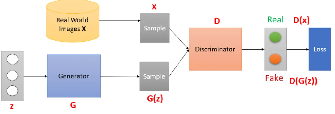
Figure 2.11: GAN architecture

Assume real data is X and the latent representation of an image is z. Dis-criminative (D) takes the sample x from real data and assign a value of 1 to it, that means it is real data and assigns 0 to 𝐺(𝑧) sample to assign fake data. Neural network G (z, θ₁) is the model mention above from generator G, it map input noisy data z to the desire data x, and other neural network D (x, θ2) models the discriminator and output probability in range 0 and

1. In both networks, θi represents the weight or parameter associated with each network [2].

2.4.2 GANs training

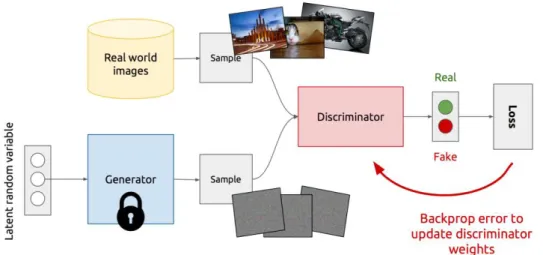
The training of both networks is in cyclic phases. In the first phase, dis-criminator D gets trained. First, the disdis-criminator start training to do cor-rectly classification of data if it is real or fake, which means its weight updates to maximize the probability that if the data come from x is a real dataset while minimizing the probability that any fake image belongs to it is not real. In the technical terms, the loss/error function used D(x) and minimize D(G(z)). The discriminator train on both real and fake and max-imize its reward my minimizing its loss. It uses Stochastic Gradient De-scent (SGD) with backpropagation. At this stage, the generator does not get trained.

(26)

Figure 2.12: Discriminator training

In the second phase, generator G gets trained by the feedback from the discriminator. Now the generator is updating its weights and optimized to maximize the probability that any fake image is classified as a real one. It means its loss/error function use for this network is max D(G(z)).

Figure 2.13: Generator training

Since both networks are trying to optimize opposite loss functions like minimax game with value V (G, D). The generator is trying to maximize its output and the discriminator is trying to minimize the same value. The value function for these both will be.

𝑚𝑖𝑛𝐺𝑚𝑎𝑥𝐷𝑉(𝐷, 𝐺) = 𝐸𝑥~𝑝𝑑𝑎𝑡𝑎(𝑥)[𝑙𝑜𝑔𝐷(𝑥)] + 𝐸𝑧~𝑝𝑑𝑎𝑡𝑎(𝑧)[log (1 − 𝐷(𝐺(𝑧)))]

(2.8)

After both generator and discriminator are modeled with neural net-works, a gradient-based optimization algorithm can be used to train the GAN. As stochastic gradient descent has proven most successful in mul-tiple fields, it is also successful for GAN [2].

(27)

2.5 Depth Image-Based Rendering

3D videos are a new type of visual media that has a highly expanded user’s sensation over the 2D videos. The development of different display technologies and user expectations for 3D videos has given the researcher a new area to search for how to represent and render realistic 3D impres-sions. A user will create a 3D depth impression for each eye to receive its corresponding view [27]. The 3D impression is attractive in applications such as imaging [28] [29], multimedia services [30], and 3D reconstruction [31].

Projective geometry is a known mathematical framework in computer vi-sion. Projective geometry applications include scene reconstruction, ro-botic navigation, and modeling perspective projection of 3D. In perspec-tive geometry, two parallel lines meet at infinity, and equations in the perspective geometry use homogenous coordinates. This provides a way to create (𝑁) − 𝐷 vector to (𝑁 + 1) − 𝐷 in perspective space. For example, a point in 2𝐷 image with a 2𝐷 can be represented 3𝐷. As a consequence, equations become linear and can be expressed by using matrix operation in perspective projection.

Figure 2.14: Camera model: (a) Projections illustration; (b) Geometric relations [13]

Let the camera center C be placed at the origin of the coordinates system the optical axis be collinear with the z-axis. The geometrical relationship between the 3D world point 𝑀 = (𝑥, 𝑦, 𝑧)𝑇 and the image point

𝑚 = (𝑢, 𝑣)𝑇_{in the image, the plane is [13].} 𝑓 𝑧

=

𝑢 𝑥

=

𝑣 𝑦 (2.9)

(28)

𝑢 =

𝑓𝑥

𝑧

, 𝑣 =

𝑓𝑦

𝑧

The transformation from world points to camera coordinate.

𝑧 (

𝑢

𝑣

1 ) = [

𝑓

0

0 𝑓

0

1

0

0 ] (

𝑥 𝑦 𝑧 1

)

(2.10)

Where 𝑢 and 𝑣 are the coordinates of pixel m in the image. The above matrix transforms the world coordinates to the image coordinates which is known as the projection matrix. The simple form of the above matrix is [13].

𝑧𝑚 = 𝑃𝑀

(2.11)

Where 𝑀 = (𝑥, 𝑦, 𝑧)𝑇and 𝑚 = (𝑢, 𝑣)𝑇 are the homogenous coordinate of 3D world points and its projection of the camera on the image plane. P is the projection matric of the camera and contains information about focal length and real cameras are defined such as position and orientation to world coordinates frame. The 3D world point to the 2D image point is the transformation of the world point to the camera point and then the image point. For the camera, C world coordinates frame is transformed to center camera C coordinates frame can be expressed 𝑀𝑐𝑎𝑚 = 𝑅. (𝑀 − 𝐶), where 𝑀𝑐𝑎𝑚, M is the same world points to the camera coordinates and world coordinate frame. After simplification by using homogenous coordinates, the camera matrix becomes

𝑃 = 𝐾{𝑅|𝑡}

(2.12)

Where

{𝑅|𝑡}

is the extrinsic parameters matric and 𝐾 is the intrinsic cam-era calibration matrix. The extrinsic describe the camcam-era location and ori-entation transformation from the world coordinates to camera coordi-nates. R is the rotation matrix, and t is the transformation vector. The in-trinsic camera calibration matric transform camera coordinates to the pixel coordinates [13]. It describes the properties of lenses, image sensor, focal distance 𝑓, skew parameters 𝑠, image center 𝑜𝑥𝑜𝑦, and camera pixel size 𝑠𝑥𝑠𝑦 in 𝑥 and y directions its matrix defined as [13]:

(29)

𝐾 =

[

𝑓 𝑠𝑥

𝑠

𝑜

𝑥

0

𝑓 𝑠𝑦

𝑜

𝑦

0

0 1 ]

(2.13)

In general projection equation written as

𝑧𝑚 = 𝑃𝑀

(2.14)

Where 𝑧 is the distance between the world point and focal plane, P is the projection matrix.

Depth Image Based Rendering (DIBR) is generally used to generate vir-tual views in free point television and 3D [32]. From original cameras few images at different viewpoints various 3D views can be generated. The main principle for generating new views is projective geometry, where the 3D geometry of original images as well as its camera location in form of extrinsic and intrinsic camera parameters, should be known [33] [34]. Depth information of image includes its MVD data, mapping of image content into 3D scene space into a virtual camera view can be conducted [34]. Figure 2.15 shows the scene that is visible to the original cameras are marked as a horizontal line. Those visible to virtual cameras are marked with diagonal lines. There are uncovered areas visible to the virtual cam-era but invisible to the original camcam-eras must be reconstructed syntheti-cally [33].

(30)

Figure 2.15: Virtual camera view from original cameras [33]

Depth Image Based Rendering (DIBR) is a technology for synthesizing virtual images at different viewpoints using the original image and its depth map. There is some issue with virtual images that some areas which are invisible in real cameras can become visible in virtual ones. This is problematic in case of extrapolation beyond the baseline of the original image [33] To overcome this problem in the synthetic view there are some existing methods to address the disocclusion problem. The first one is the missing image region is replaced by some color information [35] and the second approach is depth map pre-processed in such a way that no disocclusion occurs in the rendered image [36].

(31)

Figure 2.16: DIBR system block diagram [37]

figure 2.16 illustrates the depth image-based rendering for advanced 3D TV. It consists of three parts pre-processing of Depth Image, 3D Image wrapping, and hole filling. First smoothing filters are applied to smooth the depth image and then the wrapper generates the left and right view according to the smooth depth map and nearest view. If there are still left holes, the hole filling method applies [37].

2.6 Related Work

In [13], Suryanarayana M. Muddala addresses the problem of DIBR to improve the quality of rendered images. The author’s goal is to build a solution that tackles the problem of DIBR. To fulfill that purpose author presented different approaches that improve the quality of the image. A direct approach with one-dimensional interpolation is called the edge-aided used to improve the quality of the image. The disocclusion is han-dled with a depth-based inpainting method that reconstructs the missing part in the virtual view.

In [38], Cheng and others discuss a new algorithm that developed for inpainting of disocclusion in-depth image-based rendering. It uses three approaches to improve the synthesis by preprocessing of the depth image by using bilateral filters, by filling the disocclusion with preserving the depth level and structure. Also, the trilateral filter is used which combines the spatial location and color intensity with the depth information. The Depth-aided image inpainting for novel view synthesis [39] also ad-dresses the disocclusion problem. They divided disocclusion into two-parts small and large. The small disocclusion was painted through the hole-filling method based on preprocessing techniques. Because prepro-cessing techniques have limitations and can inpaint small disocclusion so the author proposed a new inpainting technique based on texture and propagation process that retrieves missing pixels.

(32)

3 Methodology

Initially had to study different architectures and methods which can solve this problem. The GAN is chosen to inpaint disocclusion because it can get trained on a small set of data. To evaluate the output of GAN, the PSNR, and SSIM methods are used because these are standard methods to evaluate the quality of an image. PSNR compares pixel to pixel quality of the generated image and real image on the other hand SSIM compares structural similarities between two images. To achieve the required re-sults in this experiment follows some methods which are below.

• Data Preparation • GAN Training

• Inpainting on prepared data with GAN • Inpaint performance measure

• Analysis of results

Detail description of these methods is listed below.

3.1 Data Preparation

The dataset from The Interactive Visual Media group at Microsoft Re-search (MSR3DVidea-Breakdancers) [8] was used for rendering data. This data includes a sequence of 100 images by 8 different cameras who´s depth map computed from the stereo including calibrations parameters for each camera. From this 2D image dataset, 2D virtual images have been synthesized for each camera for the other seven cameras by using the Depth Image Based Rendering (DIBR) technique. For example, camera one creates virtual images for all other cameras for each it will create 100 images and it shall create a total of 700 images. All eight cameras generate 5600 virtual images from their relative ground truth and provided cali-bration parameters for all cameras. figure 3.1 is an example of two cam-eras ground truth and depth map.

(33)

Figure 3.1: Ground truth and depth map of an image of Cam 1

Figure 3.2: Ground truth and depth map of an image of Cam 7

3.2 GAN Training

Generative Adversarial Network (GAN) architecture is design has two neural networks (discriminator and generator). The real dataset MSR3DVidea-Breakdancers [8] is input for the discriminator and the DIBR generated dataset is input for the generator. Both networks such as in figure 3.3 get the training on the DIBR generated dataset as GAN cessing described in the literature section. figure 3.3 describes the pro-posed architecture of GAN, where the generator takes DIBR generated images dataset as input and whereas the discriminator takes the real da-taset for training to validate between real and fake. Figure 3.3 shows the architecture of GAN, where z is the latent representation of the image.

(34)

Figure 3.3: Proposed GAN architecture

3.3 Disocclusion inpainting with GAN

The DIBR generated dataset will be inpainted by the training of GAN. GAN can become capable of inpainting disocclusion that occurs during the DIBR process. After the training GAN produces such images that do not have any disocclusion. If the GAN results are not as desired there is another method that combines the DIBR image and GAN image. It means this method replaces the missing pixels of the DIBR image with GAN’s generated nonoccluded pixels image. GAN and GAN plus DIBR methods are used to inpaint disocclusion in generated data.

3.4 Inpainting performance measure

For measuring the inpainting performance of the GAN and filled method, Peak Signal to Noise Ratio (PSNR) [11]and Structural Similarity Index (SSIM)[12] methods are used. These are the standard methods to use to measure the performance of an image. PSNR easily define as the adjusted form of the mean square error. Mean square error measure the per-pixel difference between an original image and its new form [11]. Formally de-fined as

MSE =

1 𝑛

∑

(𝑥

𝑖

, 𝑦

𝑖

)

2 𝑛 𝑖=1 (3.1)

The PSNR formally define as

𝑃𝑆𝑁𝑅 = 10. log

₁₀

(

𝑀𝐴𝑋𝐼2

𝑀𝑆𝐸

)

(3.2)

Both methods measure the absolute error in the original image and vir-tual image. On the other hand, SSIM will use to check the perceived changes in structural information from the original uncompressed image. It is formally described as in equation 3.3.

(35)

𝑆𝑆𝐼𝑀(𝑥, 𝑦) =

(2𝜇𝑥𝜇𝑦+𝑐1)(2𝜎𝑥𝑦+𝑐2)

(𝜇_𝑥2+𝜇_𝑦2+𝑐₁)(𝜎_𝑥2+𝜎_𝑦2+𝑐₂) (3.3) By using these methods pixel to pixel difference and structural changes will be compared with the original image to DIBR generated, the original image to GAN generated the image and original to the filed method.

3.5 Analysis of results

The hypothesis to be tested is whether the above methods (DIBR-only, GAN-only, and filled) are significantly different from each other. The null hypothesis is that the means of any two distributions are equal, i.e. there is no difference. The null hypothesis will be tested by performing student t-tests. If the t-test rejects the null hypothesis, then it means that there is a statistically significant difference between the two tested distributions. To perform the t-test, first, we have to find the mean, variance, standard de-viation, and 95% confidence intervals of all the tested methods.

To calculate the standard deviation, first, one needs to find the mean of the PSNR and SSIM. To calculate the mean following equation 3.4 used, where n is the total number of images in the test set, the value 𝑥𝑖 is either the PSNR or SSIM value of image i.

𝜇 =

1

𝑛

∑

𝑥

𝑖 𝑛

𝑖=1 (3.4)

For the calculation of variance[40], one needs to compute the sum of squares of differences between all numbers and their mean where 𝜇 is mean and n is the total number of images in the test set.

𝜎

2

=

∑ (𝑥𝑖−𝜇̅)2

𝑛 𝑖=1

𝑛 (3.5)

Standard deviation [41], can be calculated by taking the square root of variance.

𝑆𝐷 = 𝜎 = √

∑|𝑥−𝜇|2

𝑛 (3.6)

For the calculation of 95% confidence interval [42] for a sample distribu-tion of size n whose standard deviadistribu-tion 𝜎 is known, the following

(36)

equa-95% 𝐶𝐼 = 𝑥̅ ± 𝑧.

𝜎

√𝑛 (3.7)

It required a statistical test to see whether the tendencies of two groups of data (images) are different from each other. For that this purpose t-test was used. To see a comparison between two groups of data used name 1 and 2 with the means (𝜇1𝑎𝑛𝑑 𝜇2), variance (𝑆12 𝑎𝑛𝑑 𝑆22) and sample size (𝑛1𝑎𝑛𝑑 𝑛2), the t-test value can be calculated through this formula[43].

𝑇 =

𝜇1−𝜇2 𝑆_𝑝2√_𝑛11+2

𝑛2

(3.8)

3.6 Libraries

Different libraries of Python have been used during this project to imple-ment the GAN. These libraries are commonly used during machine learn-ing projects. A few of these libraries are listed below

Numpy[44] is Python’s library for adding support for large, multi-dimen-sional arrays and matrices. It can perform multiple operations on arrays and guarantee efficient calculations with arrays and matrices.

Keras [45] is a library that provides a Python interface for artificial neural networks. It acts as an interface for the TensorFlow library. Its focus is on fast experimentations. Many sub-libraries of Keras are used in a project like layers, ImageDataGenerator, models, optimizers, initializers

OpenCV [46] is an open-source computer vision and machine learning library that purpose is to provide a common infrastructure for computer vision and machine learning applications.

Jupyter notebook [47] is an open-source web application that allows users to create and share code. Users can implement, run, and test the software in Jupyter notebook.

Skimage [48] or Scikit-image is a Python library designed for image pre-processing.

Time [49] library provides various time-related functions. It is also used for calculating code execution time and measuring the efficiency of code.

(37)

3.7 Hardware

A personal computer Core (TM) i7 with 16GB memory is used to execute the code on Google Colaboratory [50] or Colab. Colab is a free Jupyter notebook environment that runs in the cloud and allows you to write and execute Python code in the browser. It gives free access to GPUs with no need for configuration.

(38)

4 Implementation

This section of the report includes the implementation of methodologies that are described in the last section. Implementation of data generation through Depth Image Based Rendering (DIBR) is described in the first section, later sections include training of GAN and inpainting methods based on GAN. Implementation of performance measure and result anal-ysis describes in the last two sections respectively.

4.1 Data Preparation Implementation

For the data generation, a guideline from the Elijs Dima’s [51] and Chris-toph Fehn’s [52] are used. The DIBR produces a 2D virtual image from a 2D image and depth map. It uses horizontal parallax and a world point oriented DIBR algorithm. The synthesis image is translated horizontally only so line by line adjustment can as images are rectified. MSR3DVidea-Breakdancers provides input information like original image (RGB), the image’s depth map, camera’s calibration matrix.

Initially, do denormalization of the depth map and find the step size dis-tance and normalize it again. After that determine the direction of column iteration along the line and check the virtual view position, if its right of original then starts shifting left most pixel first. It will prevent back-ground overwriting during overlap cases. Now need to know the direc-tion of iteradirec-tions along the horizontal and have to iterate through every pixel of every row. It calculates each pixel respective world point from the original camera’s and its depth. Then calculate the virtual camera pixel position from the word points.

4.2 GAN Implementation and training

The dataset MSR3DVidea-Breakdancers [8] includes 100 images captured for every 8 different cameras with dimensions of 1024 × 768 × 3 and output of DIBR which also have the same dimensions. It is quite difficult to pass such data to GAN with such high dimensions because of its large number of parameters, it takes more time to execute. To reduce the computational time input DIBR dataset resized into 192 × 256 × 3, nearest-neighbor inter-polation is used to down-sample images[53]. This dataset contains 5600 images and for training, purpose split this data into two groups, training (x train, y train) data, and testing (x test, y test) data with an 80:20 ratio. In each group, x has generated the view, and y is ground truth. Training data contains 4480 images and testing data contains 1120 images. It is

(39)

hard to upload whole data at one therefor have divided this data into batches size of 70 and uploaded to GAN.

4.2.1 Generator Implementation

After uploading the dataset, a GAN architecture (model) is implemented which uses this data. Two separate convolutional neural networks are im-plemented which are generator and discriminator. The generator consists of a convolutional neural network as an encoder and a decoder. The en-coder part consists of Conv2D which are convolutional layer parameters, filters to determine the number of kernels to convolve with the input layer for convolutional operation, each of these operations produces a 2D acti-vation map. Then Max-Pooling is applied to reduce the spatial dimen-sions of the output. The decoder consists of Conv2D and UpSampling2D that simply double the dimensions of the input[54]. To implement the generator’s networks first need to initialize some input on which it will train. There are several convolutions performed on input data with dif-ferent filter sizes 64, 128, and 256 where kernel size is 3 × 3.

The first convolution layer performed for feature extractions and use ac-tivation function ReLu [55] for the classification. The next layer enhances features extractions and classification of the previous convolution. After feature extraction and classification Max-pooling [56] is applied for down-sampling to reduce the number of parameters also computations in the network help to control overfitting. Next Batch-Normalization [57] technique is applied to faster and more stable training of this network. The decoded part use UpSampling2D with Conv2D. For the prediction in the last convolution use the Sigmoid function[57][58].

(40)

Figure 4.1: Generator parameters summary 4.2.2 Discriminator Implementation

The discriminator is also a convolution neural network that examines the input whether is it a real image or a fake image. Discriminator takes two types of the input original one and which comes from the generator. It does multiple convolutional iterations on the input to identifies the input is real or not. Discriminator also has several convolution layers with dif-ferent filter sizes and kernel size is 3 with strides size 2 such as in figure 4.2. The generator uses the LeakyReLu activation function to solve zero slop problems, speedy training with dropout [59] 25% to overcome the overfitting problem, and Batch-Normalization to a stable network.

(41)

Figure 4.2: Discriminator model

After several iterations converted the data into one dimension and sig-moid function used for the prediction. Summary of the numbers of pa-rameters shown in figure 4.3.

(42)

Figure 4.3: Discriminator parameters summary 4.2.3 GAN Training

To train GAN, the discriminator should train first with loss function bi-nary cross-entropy and optimizer Adam [60] to update the network’s weights iteratively in data training.

(43)

The generator compiles first and at that moment discriminator’s is disabled. and discriminator

After the generator’s compilation, the discriminator gets complied.

Int the end, both are compiled together and the GAN model is ready for training.

The GAN model is ready for training now. The size of the dataset is big so the whole dataset can't pass at once as input to the GAN, because of this, the dataset is divided into batches (batch size 64). The GAN gets bet-ter with the training so initially, ibet-terations (epochs) set to 130 to get the required results. In the network, two ground truth set for valid and fake data. Then started the training of the discriminator as real data classified as ones and fake data classified as zeros and calculated the loss for both real and fake, it should be near to 100% that means the discriminator get-ting training. The generator’s training starts with the discriminator’s feed-back and it produces new images from the input. Figure 4.4 describes the above procedure.

(44)

4.3 Inpainting on prepared data with GAN Implementation

GAN’s inpainting disocclusion implementation is described in section GAN training (section 4.2.3). To generate better inpainted disocclusion image, a method is implemented which replaces the holes (occluded pix-els) of the input image (DIBR) with GAN Generated Image’s nonoccluded pixels. As in figure 4.5, the DIBR image has black holes and the GAN im-age has blurriness.

Figure 4.5: Before combining both images

For filling the missing holes in the DIBR image the below method replaces those pixels with GAN’s image the same location pixels. The result of this method is in the results chapter. Figure 4.6 describes the replacement of missing pixels with GAN image pixels.

(45)

4.4 Inpainting performance measure

To measure the performance of generated data two methods Peak Signal to Noise Ratio (PSNR) and Structural Similarity Index are used. These methods take two inputs to compute PSNR and SSIM. The first input is the ground truth image and the second input is the image for which we want to measure the PSNR/SSIM with the ground truth image. Input is either the

• DIBR image

• GAN generated image • Filled image

The execution time and average PSNR/SSIM for all test data are com-puted with the batch size 1120 images.

Standard python library "skimage" is used to compute the PSNR and SSIM and time to calculate execution time. In this part is the implementa-tion of the predicimplementa-tion of each image one by one, generate filled DIBR im-age, compute PSNR/SSIM, and compute the execution time.

Figure 4.7: Used libraries for time PSNR/SSIM computation

PSNR of DIBR image to ground truth, GAN image to ground truth, and filled image to ground truth are computed as below.

(46)

Figure 4.8: PSNR computation

Similarly, the Structural Similarity Index (SSIM) of DIBR image to ground truth, GAN image to ground truth, and filled image to ground truth are computed.

Figure 4.9: SSIM computation

4.5 Implementation for analysis of results

The null hypothesis is used to measure statistic accuracy. To draw the plot, the distribution of PSNR and SSIM for each image type DIBR image, GAN image, and filled image are drawn. First of all, PSNR is measured for all image types. In the second step mean and confidence intervals are calculated for each and then a stack PSNR for 95% confidence intervals. The pairwise t-test is used for each measurement (PSNR, SSIM) to check the statistically significant difference and structural similarities between the different methods DIBR, GAN, and filled. In figure 4.10 and figure 4.11 is the example of the code for the t-test for PSNR, similarly, it is cal-culated for SSIM.

Figure 4.10: T-test for PSNR

(47)

5 Results

This section of the report contains the results of methodologies that are implemented in the previous section. It shows the output of DIBR mentation, GAN inpainting, filled method, and performance of imple-mented GAN with original data.

5.1 DIBR generated data

When DIBR implemented on the MSR3DVidea-Breakdancers dataset it produced a virtual dataset of 5600 images from a small dataset that has 800 images. Few produced images from the virtual dataset are shown in figure 5.1.

Figure 5.1: Virtual view from camera 1 to virtual cameras (a) Camera 2 (b) Camera 4 (c) Camera 6 (d) Camera 8.

These are results of the DIBR process from camera 1 to virtual cameras 2,4,6 and 8. There are two problems with these images, disocclusion, and scaling. Because of scaling newly generated images have a lower number of pixels. To resolve this issue a new function is implemented which workaround and solves the scaling/rotation problem.

(48)

disocclu-5.2

GAN Results

After the training, GAN produces these results from the start of training to end the training. figure 5.2, figure 5.3, and figure 5.4 show the training progress of GAN at the initial iteration, intermediate iteration, and final iteration. On the first iteration, when GAN is not trained it produces low-quality results. On the left side of figure 5.2, DIBR generated image down-sized to 192 × 256 is shown, and on the right side, GAN generated image of the same size is shown.

Figure 5.2: Output after 1st_{iteration out of 130}

When the network is half-trained it produces improved results with less blurriness.

Figure 5.3: Output after 60th_{iteration out of 130}

When GAN is fully trained it produces much better quality results. It has comparatively less blurriness as compared to half-way trained GAN.

(49)

Figure 5.4: Output after 130th_{iteration out of 130}

The training set for 130 iterations to see if there is an improvement in the accuracy of the model. After the first iteration discriminator’s loss for real and fake data is below as well as generator loss.

Output at 1st

Iteration

Real data Fake data Real and fake data

Discriminator Loss

0.296 0.216 0.256

Accuracy 92.19% 93.75% 92.97%

Table 5.1: Discriminator loss and accuracy at 1st_Iteration

Output at1st_Iteration _Dataset

Generator loss 2.303

Table 5.2: Generator loss at 1st_Iteration

Output at 60th

Iteration

Discriminator Loss

0.001 0.001 0.001

Accuracy 100% 100% 100%

Table 5.3: Discriminator loss and accuracy at 60th_Iteration

Output at 60th_Iteration _Dataset

(50)

Output at 130th

Iteration

Discriminator Loss

0.002 0.011 0.006

Accuracy 100% 100% 100%

Table 4.5: Discriminator loss and accuracy at 130th_Iteration

Output at 130th_Iteration _Dataset

Table 5.6: Generator loss at 130th_Iteration

After the 130 iterations, the discriminator is for real and fake data is zero percent and generator loss also gets better. Also after the 130 iterations generator loss again is low that means it has converged. Experiment stop after 130 iterations because there was no more convergence and also accuracy was reached 100%.

5.3 Inpainting Method Results

GAN overcomes the disocclusion problem as there are no missing pixels but the quality of the image is not very good. It has blurriness in it. To overcome this problem a ‘filling’ method is implemented that combines both DIBR and GAN generated results. This method takes a DIBR image and fills the missing pixels in it from the pixels in the GAN generated image. Figure 5.7 illustrates the method’s results are near to the ground truth image quality.

(51)

Figure 5.5: DIBR image

Figure 5.6 is the GAN generated blurred image but it does not contain any missing pixels. The filled method will handle the blurriness in GAN generated images.

Figure 5.6: GAN image

The filled method compares each pixel of DIBR and GAN and it replaces missing pixels of DIBR with pixels from the GAN generated images as shown in Figure 5.7. This method produces better quality inpainted im-ages and comparatively close to the ground truth.

(52)

Figure 5.7: Filled image and ground truth

5.4 Performance measure Results

From the image prediction to the filling of the image, Colab takes 9.65 minutes to execute on a test dataset of 1120 images. The test dataset con-tains 20% of the images in the DIBR dataset. The average execution time for each image prediction plus filling is 0.518 seconds. The results of the execution method are below.

Total execution time(seconds) Average execution time(seconds)

579.729 0.518

Table 5.7: Execution time for image prediction and filling

The PSNR statistics for the 1120 images in the test dataset are given in the following Table. The first row of the table presents the mean PSNR, while the second row contains the standard deviation of the PSNR values. The first column contains results for the DIBR method, the second column is for the GAN method, and the third column is for the filled method. Com-pared to ground truth, the mean PSNR of the DIBR method is 18.8 dB with a standard deviation of 1.86 dB for the set of 1120 test images. The GAN method achieves a better mean PSNR of 22.7 dB, while the filled method shows the best mean PSNR of 30.9 dB

Statistic DIBR GAN Filled

mean 18.8 dB 22.7 dB 30.9 dB

Standard devia-tion

1.86 dB 1.07 dB 3.32 dB

Table 5.8: Mean and standard deviation of PSNR

Similarly, the Structural Similarity Index (SSIM) values for the same size data set are presented in the table below. The mean SSIM values for the DIBR, GAN, and filled methods are 0.332, 0.548, and 0.911, respectively.

Statistic DIBR GAN Filled

(53)

Standard devia-tion

0.119 0.046 0.003

Table 5.9: Mean and standard deviation of SSIM

5.5 Analysis of Results

Statistical results of the disocclusion inpainting of different methods are listed. The 95% confidence intervals of PSNR for DIBR image, GAN im-age, and DIBR-GAN filled image are listed below. For the analysis, a test dataset consisting of 1120 images is used. These values show a positive difference in implemented methods. The below table shows the values of confidence intervals.

confidence intervals Critical value (Standard error) at 95% confidence PSNR mean (dB) PSNR_DIBR ±0.109 18.8 PSNR_GAN ±0.063 22.7 PSNR_GAN_DIBR ±0.195 30.9

Table 5.10: Values of confidence intervals and PSNR mean

The output of t-test measurements of the different methods returned value is greater than 0. This indicates that there is an improvement in the values and the null hypothesis was there wouldn’t be any improvement. These values reject the null hypothesis because it shows there is an im-provement. The filled method shows statistically best improvement from the DIBR method and the GAN-only inpainting method.

In Figure 5.8 and Figure 5.9 the plot comparison of the mean PSNR with a 95% confidence interval for the three methods is illustrated. The red line is the mean PSNR values and the blue area represents the 95% confidence intervals. The plot shows that 95% of the generated images through GAN are better than DIBR generated images, less than 5% of images of GAN can have similar quality. On the other hand, the filled method’s 95% con-fidence interval shows that 95% of filled images have a better value within the ±0.195 range. Even its worst image quality is better than GAN gener-ated images which have improved quality than DIBR

(54)

Figure 5.8: Mean PSNR and 95% confidence intervals comparison

Figure 5.9 shows the mean values of the three methods. The DIBR’s PSNR value is 18.8db, the GAN has 22.7db, and the filled method’s PSNR value is 30.9db.

Figure 5.9: Mean PSNR and 95% confidence intervals of DIBR, GAN, and filled methods

(55)

confidence inter-vals

Critical value (Standard error) at 95% confidence

SSIM mean

SSIM_DIBR ±0.0070 0.332

SSIM _GAN ±0.0027 0.548

SSIM _GAN_DIBR ±0.0031 0.911

Table 5.11: SSIM Mean and confidence intervals values

Figure 5.10 and Figure 5.11 shows the plot of the SSIM values of the three methods with a 95% confidence interval. The close values to 0 mean it does not have many structural similarities and if its close to 1 that means there are many structural similarities between the real and generated im-age. Like the PSNR plot similarly, these plot represents the mean value of SSIM in red line and the blue line represents the 95% confidence intervals of three methods. The filled method value shows that it has the best sim-ilarities between images within the ±0.0031 interval. Comparatively, GAN has fewer dissimilarities than the DIBR method. However, the value of the filled (DIBR + GAN) method shows it is very close to the ground truth with a mean SSIM value very close to 1.

Figure 5.10: SSIM Mean and confidence intervals comparison of DIBR, GAN, and filled methods

The SSIM mean value of the DIBR method is 0.332 which is closest to 0 in the three methods, which indicates more dissimilarities. GAN’s SSIM value is 0.548, which is slightly better than DIBR which means it has fewer

(56)

dissimilarities than DIBR. The filed method’s value 0.911, which is close to 1 which means it results is close to ground truth.

Disocclusion Inpainting using Generative Adversarial Networks

Master's thesis

Two years

Abstract

Acknowledgments

Table of Contents

List of Figures

Terminology

1

Introduction

1.1

Background and problem motivation

1.2

Problem Description

1.3

Tools, Requirements

1.4

Milestones

1.5

Overall Aim

1.6

Goals

1.7

Scope

1.8

Outline

1.9

Contribution

2

Theory

2.1

Machine Learning

2.2

Neural Networks

𝑥

, 𝑥

. . , 𝑥

𝑤

, 𝑤

. . , 𝑤

(2.1)

𝑖

𝑖

𝑛𝑒𝑡

= 𝑤

∗ 𝑖

+ 𝑤

∗ 𝑖

+ 𝑏

∗ 1

(2.2)

(2.3)

𝑜𝑢𝑡

=

=

= 0.593269992

(2.4)

𝐸

= ∑

(𝑡𝑎𝑟𝑔𝑒𝑡 − 𝑜𝑢𝑡𝑝𝑢𝑡)

(2.5)

𝐸

= 𝐸

+ 𝐸

(2.6)

𝑤

=

∗

∗

(2.7)

2.3

Convolutional Neural Networks

2.4

Generative Adversarial Networks

(2.8)

2.5

Depth Image-Based Rendering

=

=

𝑢 =

_(2.5)