SYSTEM IDENTIFICATION OF A WASTE-FIRED CFB BOILER : Using Principal Component Analysis (PCA) and Partial Least Squares Regression modeling (PLS-R)

(1)

SYSTEM IDENTIFICATION OF A

WASTE-FIRED CFB BOILER

Using Principal Component Analysis (PCA) and Partial Least Squares

Regression modeling (PLS-R)

SIMON FLINK

ANDREAS HASSLING

Academy of economics, society and technology Course: Degree project within energy

engineering

Course code: ERA206 Subject: Energy technology University credits: 15 hp

Program: Energy engineering program

Supervisor: Jan Skvaril

Examinator: Konstantinos Kyprianidis External supervisor: Elena Tomas-Aparició, Mälarenergi AB

Date: 2017-02-23 Email:

(2)

(3)

ABSTRACT

Heat and electricity production along with waste management are two modern day challenges for society. One of the possible solution to both of them is the incineration of household waste to produce heat and electricity. Incineration is a waste-to-energy treatment process, which can reduce the need for landfills and save the use of more valuable fuels, thereby conserving natural resources. This report/paper investigates the performance and emissions of a municipal solid waste (MSW) fueled industrial boiler by performing a system identification analysis using Principle Component Analysis (PCA) and Partial Least Squares Regression (PLS-R) modeling. The boiler is located in Västerås, Sweden and has a maximum capacity of 167MW. It produces heat and electricity for the city of Västerås and is operated by Mälarenergi AB. A dataset containing 148 different boilers variables, measured with a one hour interval over 2 years, was used for the system identification analysis. The dataset was visually inspected to remove obvious outliers before beginning the analysis using a

multivariate data analysis software called The Unscrambler X (Version 10.3, CAMO Software, Norway). The PCA was performed for all five time-periods together to provide the most accurate result possible. Correlations found using PCA was taken in account during the PLS-R modelling where models were created for one response each. Some variables had an unexpected impact on the models while others were fully logical regarding combustion theory. Results found during the system analysis process are regarded as reliable. Any errors may be due to outlier data points and model inadequacies.

Keywords: Household Waste, Incineration, MWS, PCA, PLS-R, System identification, Waste Management

(4)

PREFACE

This report is based on a study conducted as a degree project by two (bachelor degree/final year) students at Mälardalen University in Västerås, Sweden. The degree project is the final step of the Energy engineering program and is made during the, Degree Project of Energy Technology (course code ERA 206). The project was performed over the time of 18 weeks. Each student has been of equal part in the major parts of the degree project which includes the system identification process, including PCA and PLS-R modeling, an extensive literature study and drawing of a 3D model of the boiler. Several visits to the boiler located at the combined heat and power plant in Västerås were also made, along with a visit to a fuel analysis lab operated by Belab AB in Norrköping. This report has been worked on

continuously as the project has progressed, and was finalized after the system identification was completed.

We would like to sincerely thank everyone that has been part of the study, which resulted in this report, including the staff at Mälarenergi and Belab and professors at Mälardalen University. A special thank you to Elena Tomas-Aparició at Mälarenergi and our university supervisor Jan Skvaril, without whom this study would not have been possible.

Västerås, January 2017

Simon Flink Andreas Hassling

(5)

SUMMARY

The production of heat and electricity has always been a challenge for humankind, even more so in recent years. The production of power that is both cheap and environmentally friendly is not an easy task. Another modern day concern also linked to the environment and energy use is waste management. An increasing amount of household waste is produced each year, which may be a waste of energy and pollute the environment if not properly managed. One possible solution to both of these issues is to combust household waste to produce heat and electricity, the process is a waste-to-energy process and called incineration.

Specially designed and equipped industrial boilers today can effectively combust MSW to produce electricity and heat. This process reduces the need for fossil fuels and landfills, which requires a lot of land space and pollutes the environment. Incineration plays a large part in the energy market of Sweden, where the average person produced 458 kilos of waste during the year of 2013, half of which was incinerated. Large-scale industrial boilers in the EU needs to meet strict regulations regarding emissions provided in directive 2010/75 industrial emissions. Waste fueled boilers face the highest standard of regulations all the while requiring high efficiency to be economically viable. Municipal solid waste (MSW) is also an extremely difficult fuel to combust efficiently due to its heavily varying composition.

With the goal of learning the complex correlations between different variables and building a linear regression model, this study performs a system identification analysis of a MSW fueled CFB boiler located in the city of Västerås, Sweden. The boiler was commissioned in 2014 and has a maximum fuel power rating of 167 MW. Methods used for the system identification are Principle Component Analysis and Partial Least Squares Regression modeling, performed using the multivariate data analysis software The Unscrambler X. PCA and PLS-R are two methods often used in the analysis of very large sets of data. Both methods provide the relatively simple concepts of latent variable models existing in multidimensional spaces, and data being projected on to these latent variables.

Models developed during the system analysis are regarded as reliable considering their consistency with the theory and philosophy of combustion mechanics. PLS-R results for the CO show that there seems to be strong correlations between the chloride content in the fuel. A logical explanation for this is that chlorine has very high electronegativity, which means that it has a higher tendency to bond with other atoms. Carbon has lower electronegativity than chlorine, which makes the chlorine more favourable for oxygen to bond with.

Conclusions from the PLS-R performed for the N2O are that many factors play a part in the

formation of N2O and all emissions generally. The factors are among others, temperature,

fuel nitrogen content, NOx and CO formation and the presence of alkaline substances in the furnace. Sample grouping were also part of the results, the most plausible explanation for which is considered to be fuel variations.

Keywords: Household Waste, Incineration, MWS, PCA, PLS-R, System identification, Waste Management

(6)

APPENDICES

(8)

FIGURES

Figure 1 CFB-type boiler separation cyclone principle ... 8

Figure 2 Unburned fuel and CO vs Theoretical air factor ... 9

Figure 3 CO, NOx, O2 and efficiency vs Air-to-fuel ratio ... 10

Figure 5 PCA 2 ... 13

Figure 8 PCA correlation loadings example ... 14

Figure 9 Boiler 6 model ... 16

Figure 10 Steam flow and selected time periods ... 18

Figure 11 PCA correlations ... 19

Figure 12 PCA correlation loadings result ... 21

Figure 13 PLS-R correlation loadings CO ...24

Figure 14 PLS-R Predicted vs. Reference CO ... 25

Figure 15 Weighted regression coefficients CO ...26

Figure 16 PLS-R Correlation loadings NOx ... 28

Figure 17 PLS-R Predicted vs Reference NOx ...29

Figure 18 PLS-R Weighted regression coefficients NOx ... 30

Figure 19 PLS-R correlation loadings CO2 ... 32

Figure 20 Predicted vs Reference CO2 ... 33

Figure 21 Weighted regression coefficients CO2 ... 34

Figure 22 Correlation loadings N2O ... 36

Figure 23 Predicted vs Reference N2O ... 37

Figure 24 Weighted regression coefficients N2O ... 38

TABLES

Table 1 Predictor variables ... 22

Table 2 Response variables... 23

Table 3 Positive impact variables CO ...26

Table 4 Negative impact variables CO ... 27

Table 5 Positive impact variables NOx ... 30

Table 6 Negative impact variables NOx ... 31

Table 7 Positive impact variables CO2 ... 34

Table 8 Negative impact variables CO2 ... 35

Table 9 Positive impact variables N2O ... 38

(9)

NOMENCLATURE

Sign Description Unit

T Temperature °C

P Pressure Bar

CO Rökgaskanal f.

skorsten Carbon monoxide level in flue gases before chimney, PLS-R response mg/Nm³ NOx Rökgaskanal f.

skorsten Sulfur dioxide content in flue gases after boiler, PLS-R response mg/Nm³dg CO2 Rökgaskanal f.

skorsten Hydrochloric acid content in flue gases after boiler, PLS response mg/Nm³ N2O Rökgaskanal f.

skorsten Water level content in flue gases after boiler, PLS-R response mg/Nm³dg

TERMS AND ABBREVIATIONS

Abbreviation Description

CFB Circulating fluidized bed – a type of boiler circulating sand or other material with the fuel to improve performance

CO Carbon monoxide

CO2 Carbon dioxide

EEA European Environmental Agency

HCl Hydrogen chloride – formed by the combustion of chlorine present in MSW

MSW Municipal solid waste – trash or garbage, everyday items discarded by the public

N2O Nitrous oxide – not included in NOX

NH3 Ammonia – used for reducing pollutants in the flue

gases

NOX Nitrogen oxides – including Nitric oxide (NO) and

nitrogen dioxide (NO2)

PCA Principal component analysis

(10)

Abbreviation Description

RDF Refuse derived fuel – sorted and finely shredded fuel ready for combustion

SOX Sulfur oxide – including sulfur monoxide SO and

sulfur dioxide SO2

B6 The waste fueled boiler 6 located at the power plant in Västerås

WRC Weighed regression coefficient

RRC Raw regression coefficient

DEFINITIONS

Definition Description

Boiler A closed structure in which water is heated by burning a fuel, in this report always referring to large scale industrial boilers

Flue gas Products of combustion containing substances such as CO2, CO, NOX, SOX and HCl along with various particles

Incineration A waste treatment process involving the combustion of organic substances in waste materials

Pollutants When introduced into the environment, a substance that has undesired effects such as damaging the growth rate of plants or animals

System

(11)

1 INTRODUCTION

This introductory chapter provides the basis of the study, which includes background on waste management and incineration, challenges with combusting household waste and the purpose of the study along with research questions and the delimitations surrounding the study.

1.1 Background

Waste management

Waste management is a major problem in many parts of the world and in Europe. As stated in Cherubini, Bargigli and Ulgiati (2008), most developed and developing countries stands before the major challenge of collecting, recycling, treating and disposing of increasing amounts of solid waste. Some European countries such as Greece, Spain and Italy allow most of their household waste to end up in landfills according to statistics from the EEA (2013). Depositing household waste in landfills is not a sustainable waste management solution, since it requires large land areas and releases harmful substances into the environment. A study made by Kjeldsen, et al. (2010) found that water passing through municipal solid waste (MSW) landfills contained many pollutants such as dissolved organic matter, heavy metals and xenobiotic organic compounds.

In recent years in Sweden, there has been a great decline of waste ending up in landfills; the amount was cut in half between the years of 2009 and 2012 and less than 1 % of the

household waste in Sweden ended up in landfills in 2015, according to the Swedish

Environmental Protection Agency (Naturvårdsverket.se 2015a). Germany and Switzerland are two other European countries, which has an even lower percentage of waste ending up in landfills. One thing that Sweden, Germany, and Switzerland has in common and makes them so successful in reducing landfill, is that most of the countries waste is either recycled or used for incineration. The average person in Sweden produced 458 kg of waste during the year of 2013; half of this amount was incinerated in waste fueled boilers to produce electricity and district heating (Sopor.nu, 2016)

Incineration

According to Knox (2005), waste incineration is a waste treatment process where the organic substances of the waste are incinerated. Compared to landfill, incineration saves energy, space, and is more kind to the environment. Combustion of waste lowers the final mass of the waste by up to 96 %, which means that incineration does not eliminate the need for landfills but it drastically reduces the land area required. Another benefit with incineration is that when waste is allowed to decompose by itself in e.g. landfills, methane gas is naturally produced. Methane gas is a greenhouse gas over 20 times stronger than carbon dioxide.

(12)

Unless the gas is collected, which is a difficult and expensive task, it will eventually finds its way to the atmosphere and contribute to global warming.

Compared to other fuels, waste combustion releases more carbon dioxide/MWh than both coal and natural gas. However, the carbon dioxide that form during combustion of waste is widely considered carbon neutral, opposite to coal, which is a fossil fuel. This means that combustion of waste does not add more carbon dioxide to the atmosphere the same way that burning coal and oil does. This is because a large part of household waste contains many renewable materials such as paper, cardboard, fabrics, and wood (economist 2012). As discussed by Ruth (1998), using MSW as a fuel and converting it to energy can save the use of more valuable fuels thereby conserving natural resources.

Incineration being regarded as renewable has not always been the case however, in the past it was common to combust MSW without any sorting process beforehand, which was much more harmful for the environment. The unsorted waste contained many reusable, bulky and dangerous materials, which also endangered the people working at the plants. Most of these plants were merely used to reduce the wastes mass, and did not take advantage of the energy released during combustion (wrfound.org, 2009). Incineration plants today are required to meet very strict regulations regarding emissions, given e.g. in the European directive 2010/75 industrial emissions. Incineration contributes to more than 25 % of the need of district

heating in Sweden as of 2016, 15 TWh of the total usage of 55 TWh heat is produced by waste incineration plants.

Waste incineration in Sweden has steadily increased since the year 2000.The European Environment Agency (2013) says that a big reason for this is that Sweden has the heaviest taxation on landfilling in the EU. The increased cost of landfilling led to more interest for alternative option of waste management including the expansion of recycling and

incineration. The utilization of incineration in Sweden has increased immensely, even to the point that the incineration capacity quickly outgrew the MSW production in Sweden. This has led to a need to import waste from other countries, which is also a source of income for the power plants, since countries are willing to pay for someone else to deal with their waste. Only those facilities that can meet strict regulations and high requirements related to

emissions and handling of the waste can incinerate waste in Sweden. There are about 80 such plants of varying size in Sweden today. The requirements can be summarized to include the following, according to the Swedish Environmental Protection Agency (Naturvårdsverket, 2015b):

 Knowledge of what kind of waste is received for incineration.  A furnace that is specifically designed to combust waste.

 High demands for reducing pollution, which requires advanced flue gas cleaning facilities.

 Continuous measuring of the emissions of harmful pollutants, along with an annual performance test of the measuring equipment, which must be conducted by an independent third party.

Mälarenergi AB and the power plant in Västerås

Mälarenergi AB is the operator of a combined heat and power plant located in Västerås where the waste fired boiler 6 (B6) is also placed. The power plant consists of six different boilers using fuels such as oil, coal, biomass and waste. Boilers 1-4 are older and fueled exclusively with fossil fuels; today they are only kept ready for operation in case of very cold weather and

(13)

are not regularly used. Boiler 5 is fired with biomass and has previously acted as the base load boiler. Boiler 6 is the newest boiler at the plant and the only one fueled with MSW. It was commissioned in 2014 and has since acted as the base load boiler at the power plant. Together with B6, a completely new and modern waste preparation facility was built. It is placed on the same site as the boilers and is the first destination for MSW arriving at the power plant. The raw, unsorted MSW arrives and goes through the fuel preparation facility, a sorting process that shreds the fuel and removes unwanted material such as rocks, glass and metal. The result is a homogeneous fuel consisting of mostly paper and plastics called refuse derived fuel (RDF). Half of the MSW incinerated in B6 originates from the local area around Västerås while the rest is imported from inter alia England and Ireland. The completed RDF is transported through a conveyor to the boiler 6 building, where it is fed into the furnace through four different ducts.

1.2 Problem specifications

Large-scale boilers today meet a large number of strict requirements and regulation, originating from economic, efficiency and emission perspectives. MSW fueled boilers face some of the strictest regulation of all boiler types due to the large quantities of different substances present in MSW. It is also a technical challenge to combust MSW efficiently. Due to the heavily varying composition of the waste, it is very difficult to predict the combustion process and keep emissions low. An advanced flue gas cleaning facility is required to meet the emission regulations. Penalties for exceeding emission limits are mostly financial which motivated the power plants to keep their emissions as low as possible in order to increase profit.

Since waste incineration is a field where there is still a lot to learn and the boiler in question is relatively newly commissioned, it is of great value to be able to predict various flue gas characteristics based on the fuel composition or variables measured in early parts of the combustion process. There are many variables regarding the combustion process that affects the formation of flue gases in complex ways. Adding to the fact the varying properties of MSW, any insight of the combustion process is valuable for both the short and long-term advancements in waste incineration.

In this study, a system identification of a commercial boiler is performed and the correlations between different variables regarding the boiler are analyzed. The 148 different variables acquired in this study are fuel- and flue gas properties along with boiler operating variables such as temperatures and air flows. Values at different parts of the boiler process are included, e.g. flue gas properties directly after the boiler and after the flue gas treatment.

1.3 Purpose

Boiler 6 is a relatively newly constructed boiler; therefore, there is a very limited experience of how it operates in practice. The advanced design of the boiler and the flue gas treatment together with the wild difference between MSW sources means that it is not possible to generalize the performance of boiler 6 with experience from other facilities. All knowledge about the practical performance of the boiler needs to be collected through real world experiments and analysis.

The purpose of this study/degree project is to gain insight to the complex correlations between different boiler and fuel variables regarding the combustion and flue gas treatment

(14)

process in the specific case of boiler 6. The correlations will be used to build a linear

regression model from which it will be possible to predict different variables such as flue gas characteristics, depending on various inputs. The main goal of the study is that the combined results of the PCA and PLS-R models can be used to streamline the combustion process of boiler 6 and provide knowledge for the design of future MSW fueled boilers.

1.4 Research questions

RQ1: What is the significance of input variables such as bed temperatures and fuel composition etc. and how do they correlate with the output process variables of the boiler?

The output variables are specifically 4 different flue gases which are contributing to a negative effect to humans and/or the environment.

RQ2: What input variables has the largest impact on the formation of carbon monoxide, carbon dioxide, nitrogen oxides.

RQ3: What measures can be made to reduce emissions based on findings from RQ1 and RQ2.

1.5 Delimitations

This study has been conducted as a degree project and had a time limit of 18 weeks. System identification has been performed on one industrial boiler that only uses waste for fuel and oil burners for support. Measured boiler data has been provided by Mälarenergi AB and covers the time since the boilers commissioning in 2014 up until November 2016. The boiler is able to operate at either 70 % or 100 % load, this study focuses on five different time period chosen solely at a stable 100 % load. The reason being that the boiler is mostly operating at 100 % load, making this the most interesting choice for analysis. The length of the time periods is roughly one month each and PCA and PLS-R models were only made for the five time periods merged as one, rather than for each time period separately.

(15)

2 METHOD

This degree project has been made together by two students who have been working side by side for the complete length of the project. Each student has played an equal part in the major tasks of the project, which includes the following. An extensive literature study was made in order to gain knowledge about the system identification process and learn more about complex combustion mechanics. Mälarenergi AB provided the measuring data utilized for the system identification. Before being used for analysis, the data itself was visually inspected and analyzed in order to identify and remove outliers. The methods used for the system identification were Partial Component Analysis (PCA) and Partial Least Squares Regression modeling. PCA and PLS-R methods were chosen as they are able to handle large sets of data while remaining relatively simple. A multivariate data analysis software called The Unscrambler X was used to perform PCA and PLS-R modeling. Several site visits were also made to boiler 6 and the power plant where it is located, and to a fuel analysis lab in Norrköping. The visits provided in person contact with the people involved in the study and a lot of valuable knowledge about MSW as a fuel and boiler 6.

(16)

3 LITERATURE STUDY

An extensive literature study has been concluded in order to strengthen the theoretical foundation within the field of combustion technology and system identification. The most relevant literature includes scientific articles, previous studies, statistics collected by the European Environmental Agency and a compendium called “Combustion and flue gas technology”, written by MDH professor Lars Wester (2013). Most previous studies and sources referenced in this study were found using the online research database Google scholar and the online reference service Mendeley. The more detailed purpose of the literature study was to provide in depth knowledge of modern combustion technology, current research, and future development, with special focus on MSW incineration.

3.1 Combustion technology

Combustion has previously been a very dirty business and despite major progress in the field of combustion technology during the 1960's and 1970's, new problems became clearer. The oil crisis in 1973 was a wakeup call that the global energy reserves were limited, which gave rise to an increased interest in streamlining the energy industry and increase the efficiency of power plants. In addition, the consequences of combustion became more obvious, as health and environmental issues were linked to the harmful pollutants released into the air via flue gases from combustion. (H. Tsuji, A.K. Gupta, T. Hasegawa, M. Katsuki, K. Kisimoto, M. Morita, 2003) This led to more research on creating more effective and efficient boiler designs to improve combustion and reduce emissions.

Fluidized bed boilers (BFB & CFB)

A type of combustor that came into use in the 1970's is the fluidized bed boiler. Fluidization is the method of making a solid material such as sand, move from a static state into a more fluid like, dynamic state. The bed of the boiler is filled with a mix between fuel particles and sand, and as fuel particles enters the furnace, it immediately heats up and incinerates due to the high amount of thermal mass. By injecting primary air from beneath the bed, the pressure under the bed is increased to a limit where fluidization takes place. Depending on the particles density, some of the particles floats on the bed surface, while some sink to the bottom, making the sand “bubble”. These kinds of boilers are practical on a power scale from 20 MW and above.

Fluidized bed combustors are beneficial since they can be used to combust multiple different fuels, such as MSW, biofuel and coal. In addition, the bed temperature is stable and usually around 800-900 °C which is suitable in the sense that it is a good compromise between the temperatures where CO and NOx formation respectively, is the highest. This temperature

interval is also suitable for a technique used for reducing sulfur oxides. By adding limestone to the bed, it will bind with sulfur oxides and form CaSO3 and CaSO4, also known as gypsum,

instead of the harmful SOX.

There are primarily two different fluidized bed types, distinguished by the air velocity of the primary air fed under the bed. At an air velocity at around 3 m/s, the force from the

underlying air stream makes the bed start to bubble creating the so-called bubbling bed (BFB). At an air stream velocity exceeding 3 m/s, the force from the air is significant enough to change the bubbling state into a more storm like climate, where the sand and the fuel particles are swirling upwards along the boiler, having not only the flue gases leave the boiler,

(17)

but also some of the sand. This type of boiler is called a circulating fluidized bed boiler (CFB). In the following chapter, discussion of the primary difference between CFB-boilers and BFB boilers takes place. As well as a discussion of the pros and cons for each boiler type and which is most suitable in different scenarios. (Wester, 2013)

Bubbling fluidized bed boilers (BFB)

BFB boilers are usually preferred for smaller scale applications, and is suitable for combusting fuel with a relatively high moisture content and a low heating value. A full refractory lining that protects the wall from the high temperatures and velocity of the

particles covers the inside of the boiler wall. The bed is fluidized by an underlying air stream that is fed in through an arrangement of nozzles located on the bottom part of the boiler. The air stream causes turbulence which enhances the mixture of the fuel and combustion air. The amount of fuel in relation to the amount of sand is quite small, where the fuel only makes up of about 3 % of the total mass in the boiler at any time. By having a good mixture between the fuel and sand, the fuel efficiency increases due to an effective conversion of unburnt carbon to usable energy. A general value for the efficiency of a BFB boiler is usually around 90 %, which is higher than conventional grate boilers. (José & Pascual, 2011)

Fluidization occurs when the force from the primary air stream under the bed is significant enough to overcome the bed particles gravity and break through the bed surface. It is at this state when the bubbling process begins. The primary air makes up about thirty percent of the total required air for an efficient combustion. The rest is fed through secondary and or tertiary air inlets along the height of the boiler. The secondary air is fed above the bed, and adds necessary extra oxygen to the combustion, which for instance reduced the amount of carbon monoxide and assists the hydrocarbons further up the boiler to burn. The secondary air makes up for about 55 percent of the total amount of air. The tertiary air is introduced even further up in the boiler above the secondary air inlets. It is added to supply oxygen to the combustion of any potential unburnt carbon particles, which reduces the concentration of NOx and other harmful gases. (Zhang, 2013)

Circulating fluidized bed boilers (CFB)

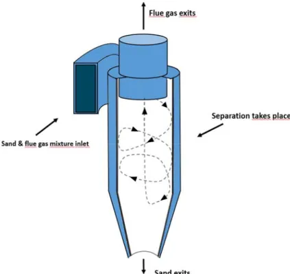
CFB type boilers are the most appropriate for large-scale applications, primarily because of its high investment cost. As the name suggest, the bed material in CFB type boilers is not restricted to the bottom of the furnace, but instead swirls around in the entirety of the boiler. Achieving the circulating effect is possible by increasing the velocity of the primary air to a point where the bed surpasses the bubbling state, which occurs at an air stream velocity of around 6 m/s. By design, a CFB boiler is very similar to the BFB boiler, but since the thermal bed covers a wide area of the boiler, the heat transfer to the cooling water reaches a higher efficiency; CFB type boilers can reach an efficiency up to 95 %. (José & Pascual, 2011) The circulating bed does present some new problems however. Due to the swirling of the sand, some of it exits the boiler along with the flue gases. To separate the sand from the flue gases, it passes through a separating cyclone. As the mix of sand and flue gases enters the cyclone, it begins to move in a helical pattern, as it is pushed toward the cyclone wall. Since the sand particles are heavier than the flue gases, it loses its kinetic energy faster as the air continues its spinning pattern. This will cause the sand and the flue gases to start separating from each other, the sand will slide downwards the bottom of the cyclone, and the flue gases begins to change direction and moves up in the center of the cyclone container. The

illustration in figure 1 shows the principles of this phenomenon in a cross section of a separation cyclone and the paths of sand and flue gas particles. (Howstuffworks.com, 2016)

(18)

Figure 1 CFB-type boiler separation cyclone principle

3.2 Emissions and combustion theory

A direct consequence of combustion is the formation of flue gases. Flue gases contains a number of substances that are each more or less harmful to either humans or the environment. Substances are e.g. different oxides (oxygen compounds), such as carbon oxides, nitrogen oxides and sulfur oxides. Different oxides have different properties, but what most of them have in common is that they are directly harmful to both humans and the environment.

Carbon Oxides – CO and CO2

The greatest byproduct from combustion are the carbon oxides, consisting mainly of carbon monoxide (CO) and carbon dioxide (CO2). Carbon dioxide is commonly known for its

contribution to the greenhouse effect, but is beyond that not directly harmful to humans or the environment as long as it is not in a concentrated state. Carbon Monoxide on the other hand poses a direct threat to humans, when inhaled; it could permanently reduce the

capability of blood to transport oxygen. In addition, it carries a risk for humans to suffer from heart diseases (Wester, 2013). Both CO and CO2 is the product of carbon released from the

fuel during combustion, which oxidizes with combustion air. The main factor regarding the formation of CO is the amount of oxygen available in the furnace during combustion. Not enough oxygen results in more CO formation and unburned fuel remaining, while too much air reduces the efficiency of the combustion. Figure 2 shows the relationship between the air factor, the amount of unburned fuel, and the O2 and CO formed in the final flue gases.

(19)

Figure 2 Unburned fuel and CO vs Theoretical air factor

Nitrogen Oxides – NOx

Nitrogen oxides (NOx) is a gathering name for nitric oxide (NO) and nitrogen dioxide (NO2), NO constitutes roughly 95 % of the total NOx formed during combustion. Nitrogen oxides contributes to the formation of ground level ozone, which has a negative effect on the lung function of humans. Symptoms for high concentration of ozone can be irritation in the respiratory system, as well as inflammatory effects. NO2 also impairs the development of the

lungs for children, which can lead to permanent health defects, for instance there are clear connections between nitrogen oxides and asthma. In very high doses, the gas is directly fatal. From an environmental point of view, nitrogen oxides are harmful in the sense that it

acidifies both land and water. It also contributes to over fertilization, which leads to a lack of oxygen in the water and harms any life in the water (Trafikverket, 2016).

The majority of NOx formed during combustion originates from the nitrogen chemically bonded in the fuel, while a small part of the NOx originates from the nitrogen present in combustion air. There are three important factors, which increases the potential of formation of nitrogen oxides, the supply or concentration of oxygen, high temperatures and the

presence of hydrocarbons in the furnace (Wester 2013). Figure 3 shows the relationship between NOX and CO formation and oxygen level. A higher fuel-to-air ratio equals more

oxygen in the combustion process. More oxygen reduces CO formation but increases NOX

formation. The efficiency of the combustion also decreases with more air, due to its cooling effect.

(20)

Figure 3 CO, NOx, O2 and efficiency vs Air-to-fuel ratio

Another nitrogen-based emission is nitrous oxide N2O, also known as laughing gas or simply

nitrous. N2O is not generally included in the term NOx but it is also an oxide of nitrogen.

Nitrous is also a greenhouse gas and has a potential global warming impact about 300 times higher than CO2, as reported by Gutierrez, Baxter, Hunter and Svoboda (2005). N2O is not

only a greenhouse gas however; it can reach the stratosphere where it may be destroyed and eventually form NO. Municipal solid waste incineration is one of the sources of human N2O

emissions; its formation varies by temperature but is generally low due to the low nitrogen content in MSW (Gutierrez, Baxter, Hunter & Svoboda, 2005)

Sulfur Oxides – SOx

Sox consists by 95 % of SO2, which is formed when sulfur-containing fuel is combusted.

Sulfur oxides shares many properties with nitrogen oxides. Exposure to environments with a high concentration of sulfur oxides, for instance high traffic areas, could lead to respiratory diseases. The environmental effects are also similar to those of nitrogen oxides, contributing to acidification and the disintegration of cultural monuments (Wester, 2013).

The amount of SO2 produced during combustion can according to Wester (2003) be reduced

by feeding chalk either to the flue gas duct or by wet or dry reactor. The chalk contains calcium, which bonds with the sulfur to produce either calcium sulfide (CaS) or calcium sulfate (CaSO4). Thus, reducing the sulfur available for oxidation. Adding chalk can also

reduce the formation of other harmful pollutants such as hydrogen chloride (HCl) and hydrogen fluoride (HF).

Hydrogen chloride – HCl

When chlorine, which is present in some fuels, is combusted it forms the acidic gas HCl. Plants, food, paper and especially plastics such as PVC, contains chlorine. The mechanics of HCl formation is that plastics polymer chain is ruptured during combustion, which results in the release of the chemically bonded chlorine, in the form of gaseous HCl. MSW is always a source of chlorine, but even if there were no PVC plastics in the fuel, there would surely be other sources, such as household chlorine, present. This means that there is always going to

(21)

be HCl present in the flue gases of incineration, which must be removed before being released in to the atmosphere. It is estimated that PVC is responsible for about half of the formation of HCl when combusting MSW, while the rest comes from wood, paper, etc. (Ciotti & Sevenster, 2013)

Acid gases such as HCl and SOX can be neutralized by adding chalk, containing the active

substance calcium. This leads to the formation of the corresponding salts of the substances instead of the acidic gases like HCl. (Ciotti & Sevenster, 2013)

Hydrogen fluoride – HF

Hydrogen fluoride is an extremely acidic gas; it is formed during combustion of fluorinated hydrocarbons, which are found in e.g. plastics. HF is a highly dangerous gas, even more corrosive and reactive than HCl; it can cause blindness to humans by destruction of the corneas. When HF is exposed to water, it forms the very toxic hydrofluoric acid, which will severely corrode glass, metals, minerals and many organic substances. (sepa.org, 2016)

3.3 Data analysis

Data analysis is an important aspect of many fields such as chemistry, medicine and chemical engineering. Chemical investigations to systems such as industrial boilers provide lots of data and we need tools to analyze these data in order to provide knowledge about the systems (MacGregor, 2002). It is important to note that a significant constraint to data analysis is that the results it present should be compliant with the theory and philosophy of chemistry. The amount of data provided by chemical systems has significantly increased between 1970 and 2001, to the point that the meaning of lots of data has substantially changed. For

example, the number of variables has increased from usually being between 5-10 variables to now being 100-1000 (Kettaneh, Berglund & Wold, 2005).

Principal Component Analysis (PCA) and Partial Least Squares regression (PLS-R) are two methods often used in the analysis of very large sets of data (Jackson, 1991)(Wold &

Josefson, 2000). The methods works computationally well for a large amount of variables and observations. Both methods provides the relatively simple concepts of latent variable models existing in multidimensional spaces, and data being projected on to these latent variables. It is an effective way for utilizing the richness of information in the data sets and summarizing it in an easy to grasp way (Kettaneh, Berglund & Wold, 2005).

Large data sets can provide a lot of knowledge but there are some serious problems with large sets of data. According to Kettaneh, Berglund and Wold (2005) there must be actions taken in the analysis of large data sets in order to avoid arriving at seriously misleading results. This may especially be a problem when just a small subset of the large data set is selected for analysis, which is a popular approach. One of the possible actions to increasing the accuracy of data analysis results, are to target outliers. Outliers are data points that are so far from the rest of the data that if they are included in the model, they will severely distort the results. All large sets of data contain outliers, which must be identified and removed from the data set before modeling may begin. Two additional problems with large data sets, described by Kettaneh, Berglund and Wold (2005), are non-linearities and model inadequacies. Many variables in large sets of data vary over a large range, which is a source of non-linearities. In the case of combustion, many variables are also dependent on each other in a non-linear way. In complicated problems that generate a large set of data, there are always going to be

(22)

(2005) puts it; there is nothing to do about this except to have diagnostics telling how wrong the model actually is. Common issues are that important variables are missing from the data and that the inputs of the model result in delayed responses.

PCA

Principal component analysis (PCA) is a general name for a mathematical multivariate method that transforms a large number of related variables to a smaller set of unrelated variables called principal components. PCA is according to Abdi and Williams (2010), arguably the most popular multivariate statistical technique and is utilized in almost all scientific fields. PCA is used to analyze a data table containing observations of several variables, which often are correlated to each other. The goal with PCA is to find the useful information in the data table and express it as a new set of variables, which are linear

combinations of previous variables and called principal components. Observations (points of data) can be projected onto these new components when they have been constructed (Abdi & Williams, 2010).

When accounting a large data set, it is very convenient to illustrate them visually as points in a graph, where each point in the graph represents a sample of data or an observation. By doing a feature selection, it clarifies what part is of particular interest in the graph by narrowing the dimensions of which the data is presented, which is within the area of the points of data, as visualized in figure 4.

By picking a direction and drawing a line, called a principal component, (PC1) that is diagonal in relation to the x & y axis and then projecting the data points onto the new line, the variance will be significantly larger than on either of the original x & y dimensions. PCA also finds another direction which is perpendicular to the PC1 dimension, creating a new principal component (PC2). By projecting the data points to the new PC axis, it is very convenient to rotate the axis and use the PC’s as new base dimensions, shown in figures 4 through 7.

(23)

3.3.1.1. Interpreting the results

The result of a PCA is a visualization as the correlation between different variables of a

dataset. A software used to compute PCA called The Unscrambler X, has the option to display multiple different visuals such as graphs and chart to help find correlations between

variables. A loadings plot shows the correlation between principal components and variables and is used to find correlations, an example is shown in figure 8. Variables diagonally

opposite to each other are negatively correlated while variables close to each other are

positively correlated. The circles represent how well the variables are explained by the model, the inner circle represents 50 % explained variance while the outer circle represents 100 %. This means that variables close to the outer ring are of great importance while those inside the inner circle can be regarded to have less of an impact on the model.

Figure 4 PCA 2 Figure 5 PCA 1

Figure 7 PCA 4 Figure 6 PCA 3

(24)

Figure 8 PCA correlation loadings example

3.3.1.2. PCA Scores

The PCA score plots every individual point of data in the sample on to a graph. This is very useful as it shows how the data points are distributed. The score plot can be used to get an overview of the samples and identify if they follow any obvious patterns, i.e. if they are grouped together or if there are a lot of outliers. The PCA score has a range between 0-1, where samples that are clustered contributes to a high score, and outliers contributes to a low score. This can later be used to evaluate the reliability of the PCA.

PLS-R

Partial Least Square Regression (PLS-R) is a mathematical method that specifies the relation between one or more dependable Y variables and a set of predictor X variables. PLS-R is also known as Projection to Latent Structures but is still the same method. PLS-R is a relatively new method and combines the qualities of Principle Component Analysis (PCA) and multiple regression. The method is particularly useful when the goal is to predict a set of variables depending on a larger set of explanatory variables (predictors) which may have a large correlation to each other (Abdi, 2007).

Abdi (2007) reports that there are two different PLS-R methods, which differ by the number of dependable (response) variables they specify. Method 1 (usually called PLS1) predicts one response variable while method 2 (PLS2) predicts multiple response variables. The main goal of both PLS-R methods is to build a linear model of the form

(1) Where Y is the dependable response value and X is the predictor variable. While equation (1) shows the principle of the simplest linear equation, the full final linear models resulting from

(25)

PLS-R can be described in the form of equation (2) below, provided by Koudadri et al. (2011).

⋯ (2)

The B values are the regression coefficients, which describes the impact a given predictor (Xn)

has on the response (Y). From equation (2), it is possible to predict the Y value by inputs of the X variables.

(26)

4 SYSTEM IDENTIFICATION

4.1 Description of the boiler

Boiler 6 (B6) is a CFB-boiler and at maximum load, has a fuel power of 167 MW. The annual fuel consumption can at the most reach 480 000 tons of household waste. The height of the boiler measures about 27m and the width is almost 12m while the depth is close to 4m. Fuel is fed to the bottom of the boiler in four separate ducts visible to the bottom left of the boiler in figure 9. Primary air is fed in under the bed of the boiler while secondary and tertiary air is added further up along the height of the boiler. Two cyclones seen to the right in figure 5 separates the bed material from the flue gases.

(27)

Fuel preparation process

Before the waste can be used in the boiler as fuel, it has to go through a sorting process, which converts the waste from a raw, unsorted product into a ready to use fuel. The waste makes its way to the power plant from afar by either trucks, ship or train. Regardless of the transportation method, all waste is dumped in a large bunker. At the bunker, there are two automated claws, which has two tasks:

1. The claws mix the waste and gives it a homogeneous mixture.

2. The claws transport the waste to the next step in the handling process.

From the waste bunker, the claws drop the material into 3 different pockets, each one having a feeding table. Here the waste is being fed into mills, which grinds the waste into a size similar to a human fist. After the mill the material falls on a conveyor belt, which moves it through a sorting process that separates metals and other unwanted heavy materials such as glass, rocks, metals and concrete. After this stage, the waste has been converted into RDF, fuel ready for combustion. It is now sent to the RDF-bunker which acts as a buffer, until the fuel is needed in the boiler. (Malarenergi.se, 2015)

4.2 Site visits

The power plant

To get an understanding of the actual appearance of the boiler, and the process of the flue gas cleaning, there has been a site visit to the power plant. The opportunity was given to have a tour around the boiler, led by one of Mälarenergi's employees. The tour had a very good learning effect, as it provided a more practical understanding of the different sections of the boiler and the combustion process.

Fuel analysis lab, Belab AB

Three times a day the personal at Mälarenergi takes a fuel sample of the RDF fuel before it is fed to the boiler. The sample is taken to analyze its properties, what different materials the fuel contains and to identify of the waste contains anything that shouldn't be in it.

Mälarenergi examines the moisture content on site, before the samples are being sent to the energy laboratory Belab AB in Norrköping. To get a better understanding of how a fuel analysis is performed, and also to learn more about the fuel in general, a visit was made to the laboratory in Norrköping.

4.3 Analysis and modeling

Data acquisition

(28)

years, since the commissioning of the boiler up until 2016. In total, this amount to close to four million cells of data in excel. After examining the dataset and removing unnecessary and faulty variables, the data was imported to The Unscrambler X for analysis. A table of the descriptive statistics of the data set is shown in appendix 1.

PCA

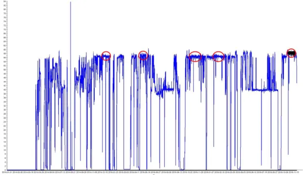
The first step in The Unscrambler X was to identify a variable which would correlate with the boiler load, in order to find time periods where the boiler was operated under relatively stable load. Steam flow was the variable chosen which was plotted in a line diagram. The steam flow visualized the boiler operation and made it possible to identify periods of stable load. Figure 10 shows what the plotted steam flow values looked like, the circled parts show the periods of stable loads which were chosen for the analysis. PCA analysis was performed for all five different time periods all together, called the global time period.

Figure 10 Steam flow and selected time periods

After a stable load period was chosen, all measured values during that time period could be analyzed using PCA. The Unscrambler X was used to perform the PCA analysis and produce multiple graph that could be interpreted to find correlations between variables. In figure 11, the most important type of graph produced by The Unscrambler X is shown.

(29)

Figure 11 PCA correlations

The graph shows all the variables and how they might be correlated. Values in opposite corners have a high chance of being negatively correlated with each other. The circles

represent how well the variables are explained by the model, the inner circle represents 50 % explained variance while the outer circle represents 100 %. This means that variables close to the outer ring are of great importance while those inside the inner circle can be regarded to have less of an impact on the model. In figure 9 we can for example see that the variables O2

and CO2 are opposite and there is also a valid explanation for why they might be correlated

which increases the probability of them being correlated in reality.

Recalculations of the PCAs were also made by first removing variables which were of the same kind i.e. multiple readings of the temperature in the bottom of the boiler. These multiple variables which showed almost exactly the same thing were not needed for the analysis and therefore complicated the PCA unnecessarily.

After recalculating PCAs they were interpreted once again. Findings about correlations between variables was used to select predictors and responses for the next step in the system identification process, the partial least squares regression modeling PLS-R.

(30)

PLS-R

There are two different methods of performing PLS-R, PLS1 and PLS2. In both methods, several predictors (X-values) are selected, the difference is the number of responses (Y-values). PLS1 analyses just one response with multiple predictors while PLS2 calculated both multiple predictors and multiple responses.

This study focuses on the use of PLS1. 64 different variables were chosen as predictors, for example temperatures, pressures, fuel composition and air flows in the boiler. The responses were as mentioned analyzed one by one and were all part of the flue gas in the flue gas duct directly after the boiler. They were as follows: SO2, HCl, H2O, NH3 and O2 at the cyclone. The

Unscrambler X was used to perform the PLS-R analysis using the mentioned predictors and responses.

(31)

5 RESULTS AND DISCUSSION

5.1 Principle Component Analysis

To provide the most accurate result possible, the PCA was performed for all five time-periods together. The PCA plot shown in figure 12 represents a summation of the data from all of the selected time periods 1 through 5. This plot is mainly used to find correlations between different variables and to get clues as to which of the variables should be predictors and responses in the next step of the system analysis, which is the PLS-R model.

(32)

5.2 PLS Regression

This chapter presents all the results concluded by the PLS regression modelling. Each selected response variable is presented in its own sub-chapter from 5.2.1 to 5.2.5.

Predictors and responses

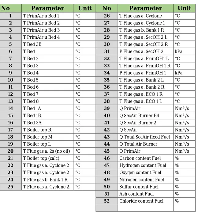
60 different variables were chosen as predictors for the PLS-R model, while 13 responses were selected. The reasoning behind the selection comes from combustion theory and results of the PCA. Table 1 show all selected responses while table 2 shows the responses.

Table 1 Predictor variables

No

Parameter

Unit

No

Parameter

Unit

1 T PrimAir u Bed 1 °C 26 T Flue gas a. Cyclone °C

2 T PrimAir u Bed 2 °C 27 T Flue gas a. Cyclone 1 °C

3 T PrimAir u Bed 3 °C 28 T Flue gas b. Bank 1 R °C

4 T PrimAir u Bed 4 °C 29 T Flue gas a. SecOH 2 L °C

5 T Bed 3B °C 30 T Flue gas a. SecOH 2 R °C

6 T Bed 1 °C 31 P Flue gas a. SecOH 2 kPa

7 T Bed 2 °C 32 T Flue gas a. PrimOH1 L °C

8 T Bed 3 °C 33 T Flue gas a. PrimOH 1 R °C

9 T Bed 4 °C 34 P Flue gas a. PrimOH 1 kPa

10 T Bed 5 °C 35 T Flue gas a. Bank 2 L °C

11 T Bed 6 °C 36 T Flue gas a. Bank 2 R °C

12 T Bed 7 °C 37 T Flue gas a. ECO 1 R °C

13 T Bed 8 °C 38 T Flue gas a. ECO 1 L °C

14 T Bed 1A °C 39 Q PrimAir Nm³/s

15 T Bed 1B °C 40 Q SecAir Burner B4 Nm³/s

16 T Bed 3A °C 41 Q SecAir Burner 2 Nm³/s

17 T Boiler top R °C 42 Q SecAir Nm³/s

18 T Boiler top M °C 43 Q Total SecAir fixed Fuel Nm³/s

19 T Boiler top L °C 44 Q Total Air Burner Nm³/s

20 T Flue gas a. 2s (no oil) °C 45 Q PrimAir Nm³/s

21 T Boiler top (calc) °C 46 Carbon content Fuel %

22 T Flue gas a. Cyclone 2 °C 47 Hydrogen content Fuel %

23 T Flue gas a. Cyclone 2 °C 48 Oxygen content Fuel %

24 T Flue gas b. Bank 1 R °C 49 Nitrogen content Fuel %

25 T Flue gas a. Cyclone 2.. °C 50 Sulfur content Fuel %

51 Ash content Fuel %

(33)

Table 2 Response variables

No Variable Description Unit

1 CO Rökgaskanal f. skorsten Carbon monoxide level in flue gases before chimney mg/Nm³ 2 NOx Rökgaskanal f. skorsten Sulfur dioxide content in flue gases after boiler mg/Nm³dg 3 CO2 Rökgaskanal f. skorsten Hydrochloric acid content in flue gases after boiler mg/Nm³ 4 N2O Rökgaskanal f. skorsten Water level content in flue gases after boiler mg/Nm³dg CO

The plot in figure 13 shows the correlation loading of the different predictors. The variables contributing to the greatest impact is highlighted with a circle. There seems to be strong correlations between the chloride content in the fuel. A logical explanation for this is that chlorine has very high electronegativity, which means that it has a higher tendency to bond with other atoms. Carbon has lower electronegativity than chlorine, which makes the chlorine more favourable for oxygen to bond with. So as the oxygen has a greater potential to bond with the chlorine rather than the carbon, the oxygen content in the combustion air could get insufficient, and therefore more CO is formed.

The CO also correlates negatively with variables such as the bed temperatures of the boiler. This would be expected, as the temperature of the combustion is one of the key factors for CO formation. An increase in the combustion temperature contributes to a lower concentration of CO formation, according to basic combustion theory. (chemguide.co.uk, 2013)

(34)

(35)

The PLS-R for the CO shown in figure 14 provided an acceptable value of explained variance. There are quite a few outliers affecting the result, most of the samples does follow a linear pattern. With a bit more effort, further investigation could be put to the narrowing of outliers and receive an even better result, but as the explained variance is within acceptable limits, no further effort will be made as of this time. The potentiality of improvements will instead be suggested for further work and is a task to be taken into account for the future.

The diagram in figure 14 below presents the regression coefficients of the predictor variables, where those who has a positive impact on the CO concentration is listed as positive value on the y-axis, and the variables who has a negative impact, is listed as negative. Those variables which had a very little impact is marked as blue, and if there would be any interest of a continued work on this project, these blue marked variables could be removed, and the PLS-R recalculated. As the diagram shows, the weighted regression coefficient displays the NH3

concentration in the flue gas duct to have the greatest positive impact.

(36)

On the opposing side of the diagram, the NOx in the flue gas has a negative impact on the regression model. As the correlation loading plot in figure 15 shown below, the chloride content of the fuel does have a great impact on the CO, and it has been proven that the impact indeed is negative. (chemguide.co.uk, 2013)

Figure 15 Weighted regression coefficients CO

Table 3 below presents the raw regression coefficients (RRC) of what the model has identified as the most positive impact variables. According to the result, the nitrogen content of the fuel is the highest impact variable to the formation of CO. According to PhD student Johanna Aurell, carbon monoxide is a byproduct of when hydrogen cyanide (HCN) binds with oxygen to form NCO + H, and will eventually react with NO to form N2O + CO. The primary air flow

will also play an important role, as it delivers oxygen to the combustion. Table 3 Positive impact variables CO

Fuel Nitrogen Content 0,677

NH3 Flue gas duct after boiler 0,202

Q PrimAir 0,099

Fuel Ash Content 0,091

(37)

Regarding what factors that has the highest negative impact on the CO formation, the sulfur content in the fuel plays an important role. This could be explained as both sulfur and carbon has the same value of electronegativity on the Pauling scale. By having the same amount of electronegativity, both elements has the same potential to bond with oxygen. This would mean that the carbon has to compete with the sulfur of the available oxygen, and thus reduce the amount of CO formed.

A similar explanation can be used for the chlorine content of the fuel. However in this case, chlorine has a higher electronegativity than both sulfur and carbon, meaning that the chlorine is more favorable to bond with, and thus do not have to compete at the same level with the sulfur, and wherefore has a lower impact on the CO formation.

Table 4 Negative impact variables CO

Sulfur content fuel ‐2,518

Chlorine content fuel ‐1,267

Hydrogen content fuel ‐0,329

Q SecAir Load.Br2 ‐0,283

(38)

NOX

The loading graph resulting of the PLS-R with NOx as a response is shown below in figure 15.

NOx is shown as a red dot and appears to be positively correlated to several of temperature

related variables. Airflows also has some positive correlations, as well as the N2O

concentration in the flue gas.

In the third quadrant, it is possible to read the negative correlations, where the chlorine content of the fuel, as well as the concentration of ammonia appears to play an important role. These findings will be discussed later on in this chapter.

(39)

Figure 17 shows that there is quite a few outliers in this PLS-R. This may lead to inaccuracies in the model. The score is however within acceptable limits, and no further improvements will be made as of this time, but will instead be left as a suggestion of improvements for the future. The graph does display that according to the data set, NOx is an unstable molecule which can have large changes in formation rate depending on ongoing operating conditions.

(40)

It is shown in figure 18 that some variables have a high negative impact on the model while some has a high positive impact. General conclusion is that temperatures have a mostly positive impact while pressure contribute with a negative impact.

Looking at the wighted regression coefficients, the concentration of NH3 is a decisive variable

in the reduction of NOx in flue gases, which is what to expect as the NH3 is beeing added for

that purpose. As for the positive contributer to NOx, temperatures seems to play a role for the WRC. This would realistic as temperature does play a role in the formation rate of NOx, but it should not play an important role for the final model, as the combustion temperatures of Boiler 6 doesen´t achieve high enough temperatures for thermal NOx to be any important contributor.

Figure 18 PLS-R Weighted regression coefficients NOx

It is not very surprising to discover that the secondary air flows are being a top contributor to an increase in NOx shown in table 5. What is surprising however, is that the nitrogen content of the fuel does not appear as any of the most impactful variables, which contradicts what was earlier discussed in chapter 3.2.2.

Table 5 Positive impact variables NOx

Q SecAir Load.Br2 0,951428

Oxygen content fuel 0,66453

Hydrogen content fuel 0,346133

Q SecAir 0,244781

(41)

According to our model, the chloride content of the fuel has the greatest negative impact on the formation of NOx in the combustion process, having a RRC of -5.8. According to PhD student Johanna Aurell (2008), a number of studies has been made investigating the impact that chlorine has to the NOx formation, where some of these studies have found obvious correlations between the two. In a series of experiments performed by Eva-Lena Wikström, she investigated seven different fuel, each with a varying chlorine concentration that ranged between 0.12 to 1.72 %. According to her results, the chlorine concentration of a fuel does not contribute to a significant increase in NOx, until it reaches a threshold of around 1.7 %, where values exceeding that having a large impact on the NOx formation (Aurell, 2008)

As for our current model, the chlorine content of the fuel has an interval that ranges between 0.47 to 0.87 %, and should therefore not have chlorine as a positive contributor to the

formation of harmful emissions. As our result proposes the opposite, where the chlorine content is instead resulting in a decrease in NOx. The explanation is likely to once again be related to the similarities of the level of electronegativity in nitrogen and chlorine. Both are having a score of 3 on the Pauling scale, and therefore makes chlorine a contester to the available oxygen. In a conversation with the staff of Mälarenergi (2016), they informed that the ammonia is being added in the transition between the boiler and the two cyclones. The ammonia is being used as a scrubber to reduce the NOx, and does explain the negative impact on the result of NOx.

Table 6 Negative impact variables NOx

NH3 FG‐Duct a. boiler ‐4,259

O2 flue gas duct b. chimney ‐3,285

SO2 flue gas duct b. chimney ‐0,796

(42)

CO2

There has been a selection of variables for the model made for the CO2. According to our

model, selecting only 19 variables was sufficient to achieve an impressive score of explained variance. These remaining variables has been selected based on the fundaments of

combustion theory, where the variables are directly connected with the three necessary properties for incineration, temperature, oxygen and fuel. This was made to reduce the amount of variables that had a low, or close to none impact on the process, and provides a greater focus on what actually is important. Figure 19 shows a clear negative correlation between the concentration of the CO2 and the amount of oxygen in the flue gases. This is an

expected finding, as the oxygen and CO2 are directly connected to each other.

(43)

When choosing predictor variables for the CO2 model, it was sufficient to select a lot fewer

variables, and still achieve an impressive score with over 90 % explained variance with only 19 variables. The sample points are following a close to linear pattern and indicates a good quality of the measurements, seen in figure 20. It is worth to note is that the CO2 is measured

as a percentage of the total emissions leaving the plant chimney.

(44)

For the weighted regression coefficients of the carbon dioxide, the result shows that the oxygen rate in the flue gas is the largest cause for CO2 reduction. As a second source of

reduction, the chlorine content of the fuel plays a similar role as for previous findings. The most important variables that has a positive impact on CO2 is in this case the

temperature at the top of the boiler, and the sulfur content of the fuel.

Figure 21 Weighted regression coefficients CO2

Table 7 show that the sulphur content of the fuel has the most positive impact on CO2

formation, more than ten times the impact of the second most important variable, air flor of secondary air.

Table 7 Positive impact variables CO2

Sulfur content fuel 3,014

Q SecAir LoadBr2 0,274

Hydrogen content fuel 0,191

Ash content fuel 0,088

(45)

The regression model presents the hydrogen content in the fuel as the greatest reducer of CO2, shown in table 8. There has been quite a difficulty to gain theoretical support for this

finding, but speculations have taken us to a phenomenon called The Sabatier reaction, which is a reaction discovered by French chemist Paul Sabatier. In this reaction, at elevated

temperatures, CO reacts with 4H2 molecules to form CH4 (methane) and 2H2O. (VanderWiel

et. al, 2002)

According to basic combustion theory, in stochiometric combustion, there wouldn´t be any unbound oxygen left in the flue gas, as it should have either converted into CO2 or have

bonded with some other molecule. As stochiometric combustion is practically impossible, it will in every case of combustion remain a portion of oxygen left in the flue gas. As the carbon failed to bond with the oxygen, it would be logical to assume that oxygen in the flue gas would have a negative effect.

Table 8 Negative impact variables CO2

Nitrogen content fuel ‐1,359

O2 flue gas b. chimney ‐0,998

Q SecAir ‐0,028

(46)

N2O

Gutierrez, Baxter, Hunter and Svoboda (2005) states that the N2O formation in incinerators

vary according to temperature and that materials with high nitrogen content such as leather and plastics would be expected to increase N2O emissions. Figure 22 show a generally

negative correlation with the fuel chloride, sulfur, carbon and even nitrogen content. An assumption could be made that higher quantities of substances other than nitrogen in the fuel would lead to a decrease in N2O emission, true to the graph. The slightly negative

correlation between N2O and nitrogen may be a result of N2O being measured before the

chimney, meaning that it has been through the flue gas cleaning facility, resulting in the unexpectedly negative correlation to fuel nitrogen content. It may also be mentioned that the fuel nitrogen content is relatively close to the middle of the graph meaning it is not well explained by the model and its result should not be too closely considered.

SYSTEM IDENTIFICATION OF A WASTE-FIRED CFB BOILER : Using Principal Component Analysis (PCA) and Partial Least Squares Regression modeling (PLS-R)