CourseScheduler

(1)

СОФИЙСКИ УНИВЕРСИТЕТ “Св. Климент Охридски”

Факултет по Математика и Информатика

ДИПЛОМНА РАБОТА

Тема: MyCourses – Система за изтотвяне на

график на лекциите в университет

Дипломант:

Теодора Проданова Пулева, ФН М22333

Научен Ръководител: Томас Левек, Университет

„Малардален“, Швеция

Консултант:

доц. Силвия Илиева,

катедра „Софтуерни технологии“, ФМИ

2010  София

(2)

MASTER THESIS IN

COMPUTER SCIENCE

15 CREDITS, ADVANCED LEVEL

School of Innovation, Design and Engineering

MyCourses – A Course

Scheduling System

Teodora Puleva

Date: September 2010

Advisor at MDH: Prof. Ivica Crnkovic Examiner: Thomas Leveque

(3)

(4)

iii

SUMMARY

Course timetabling is a time consuming problem that arise every year in each university. This is a problem that deals with assigning a large number of courses to a limited number of rooms and timeslots while satisfying a set of predefined constraints. Most of the existing timetabling systems can only be used at the university involved in the research, as each university has its own needs and requirements that differ specifically. MyCourses software tries to make a difference by allowing each university to configure which scheduling rules to use. It provides a way to schedule courses for a whole semester rather than on weekly basis. It also gives teachers the ability to easily specify their preferences, faculty members to enter various university data and also provides an optional way for scheduling university courses. The MyCourses’s automation solver uses Simulated Annealing as an optimization technique for solving the NP hard scheduling problem. Simulated Annealing searches for a better solution as well as it has advantage to escape from local minimum by allowing to move to worse solution in comparison with other algorithms which always seeks a better one.

(5)

iv

Chapter 6 TECHNOLOGIES 34 6.1 Server-side Technologies ... 34 6.1.1. .Net Platform ... 34 6.1.1.1. .Net Framework ... 35 6.1.1.2. Microsoft SQL Server ... 42 6.2 Client-side Technologies ... 42 6.3 System Requirements ... 46 Chapter 7 SOLUTION 47 7.1 Database Design ... 47 7.2 Class Diagrams... 50 Chapter 8 IMPLEMENTATION 55 8.1 Architecture ... 55

Chapter 9 TEST PLAN 67 9.1 Goal ... 67

(6)

v 9.2 Scope ... 67 9.3 Testing Strategy ... 67 9.4 Test Schedule... 68 9.5 Tools ... 72 Chapter 10 CONCLUSIONS 74

Chapter 11 FUTURE WORK 76

Chapter 12 ACKNOWLEDGEMENTS 77

(7)

vi

TABLE OF FIGURES

FIGURE 1 LOCAL AND GLOBAL MINIMAS OF A FUNCTION 2

FIGURE 2 SOFTWARE DEVELOPMENT LIFECYCLE OF MYCOURSES PROJECT 5 FIGURE 3 BRIEF OVERVIEW OF THE PROJCT PLAN FOR MYCOURSES'S PROJECT 8 FIGURE 4 MYCOURSES USE CASE DIGRAMS. MAIN ACTORS ARE ON THE LEFT SIDE, WHILST ALL

OTHERS ARE ON THE RIGHT SIDE. 14

FIGURE 5 SIMULATED ANNEALING ESCAPING FROM LOCAL MINIMUM BY CHAOTIC JUMPS. (57) 27 FIGURE 6 FLOW CHART OF SIMULATED ANNEALING’S STRUCTURE (58) 29

FIGURE 7 THE PROCESS OF CALCULATING NEXT SOLUTION 31

FIGURE 8 PSEUDO-CODE OF SIMULATED ANNEALING 33

FIGURE 9.NET PLATFORM 35

FIGURE 10 .NET FRAMEWORK 4.0 36

FIGURE 11 LINQ ARCHITECTURE (33) 38

FIGURE 12 T4 TEMPLATE THAT GENERATES CLASS WITH NAME SPECIFIED IN FIELD CLASSNAME. 41 FIGURE 13 GENERATED CLASS WHEN THE ABOVE T4 TEMPLATE IS SAVED. 41

FIGURE 14 SAMPLE HTML DOCUMENT. 43

FIGURE 15 SAMPLE STYLE FOR BODY ELEMENT. 43

FIGURE 16 SAMPLE JAVASCRIPT FOR ACCESSING QUERY STRING PARAMETERS. 44 FIGURE 17 SAMPLE JQUERY USED FOR COLLAPSING PAGE CONTENT. 44 FIGURE 18 SAMPLE JQUERY OBJECT USED FOR VISUALIZING TIMETABLE IN MYCOURSES. 45 FIGURE 19 SAMPLE CALL OF SERVER-SIDE METHOD FROM CLIEN-SIDE. 46 FIGURE 20 MYCOURSES USERS HIERARCHY. USERS ENTITY STORES DATA COMMON FOR ALL SYSTEM

USES. LECTURER ENTITY STORES DATA SPECIFIC FOR LECTURER. STUDENT ENTITY STOERS DATA

SPECIFIC FOR A STUDENT. 48

FIGURE 21 MYCOURSES DABASE STRUCTURE 49

FIGURE 22 USERS CLASS DIAGRAM 51

FIGURE 23 PROGRAMS AND COURSES CLASS DIAGRAM 52

FIGURE 24 SCHEDULE CLASS DIAGRAM 54

FIGURE 25 MYCOURSES ARCHITECTURE 56

FIGURE 26 REPOSITORY PATTERN INCLUDING A CONCRETE IMPLEMENTATION FOR COURSE ENTITY. 57

FIGURE 27 COURSE SPECIFIC REPOSITORY 58

FIGURE 28 COURSE SPECIFIC STATIC REPOSITORY 58

(8)

vii

FIGURE 30 SAMPLE METHOD FOR RETREIVING ALL ACTIVE COURSES. 61

FIGURE 31 MYCOURSES HOME PAGE. 62

FIGURE 32 MASTER PAGES HIERARCHY. BASE.MASTER CONTAINS THE COMMON ELEMENTS FOR ALL PAGES. SCHEDULE.MASTER CONTAINS THE SIDE MENU SPECIFIC FOR COURSE SCHEDULING PAGES. MYCOURSES.MASTER CONTAINS THE SIDE MENU THAT IS COMMON FOR ALL OTHER

PAGES. 63

FIGURE 33 CONTEXT MENU 64

FIGURE 34 ACCORDION MENU 64

FIGURE 35 MYCOURSES'S SCHEDULE 65

(9)

1

INTRODUCTION

University course scheduling is a tedious and error-prone task. Each year a large number of universities are facing this time-consuming task – scheduling courses. For this reason automatic timetabling software would be very useful for universities. There are various applications that currently exist, but they can be used only in the university involved in the research, as each university has its own needs and requirements that differs specifically. If such software, that only specify the list of supported constraints without the ability to switch on and off some of them, is used, the university might end up having courses scheduled according constraints that are not applicable in the university. For example, some universities allow a lecturer to teach more than one class at the same time, while most of the existing applications have a constraint that limits those classes to be scheduled together. If the application does not allow the university to set the corresponding constraint as inactive, then those courses will not be scheduled at the same time. That is why, designing and implementing an automation solver satisfying university needs in a flexible way is an important task. Using such a system in the universities can save a lot of time and effort for the program administrators and program managers who are involved in creation and management of course schedules. Also, it will save time for the lectures when requesting their preferences and availability.

There is also a wide variety of fields where timetabling problem arise including employee timetabling, examination timetabling, transport timetabling and many others. All these kinds of timetabling problems share similar characteristics. Because most of them have very specific requirements and they are very hard to be solved, a general solution of the problem does not exist. In particular, course timetabling is part of the whole timetabling problem. It has

(10)

2

been extensively studied for over 35 years and some limited success has been reported. During this time various approaches have been studied and some of them are graph colouring, backtracking, heuristic algorithms, and local search algorithms such as genetic algorithms, tabu search and simulated annealing algorithm. Each of them aims to minimize the conflicts in a schedule.

The process of minimizing the conflicts can be formulated as an optimization problem which seeks to minimize the value of the cost function. A cost function is a function that represents the constraints being violated. For solving the current course scheduling problem the Simulated

Annealing algorithm was chosen. It is a local search algorithm that has the advantage to escape from local minima compared to algorithms that always search for better solutions such as Hill Climbing, because the cost of a solution can increase as well as decrease. If the algorithm got stuck at a local minimum, it means that it has found the lowest value of the cost function for a limited range, but the optimization needs to continue until it finds the lowest value for the whole range of solutions, e.g. the global minimum. Figure 1 illustrated the difference between the local and global minima of a function. Simulated Annealing algorithm starts from a random point and gradually reduces the search radius around minima that is found. Periodically, the solver will reset and start searching a wider radius allowing the algorithm to jump out of local minima and find the global minima. As a result the algorithm finds an optimal solution or one that is as close as possible to the optimal.

One of the main objectives of MyCourses project was to develop an automation solver that finds qualitative and feasible solution. Another objective was to provide a user friendly interface that allows users to easily modify and maintain the schedules proposed by the solver. The solver’s configuration (i.e. active constraint, prioritizing them, entering required input data) should also be exposed to the administrators and other involved participants in a way that is

global minimum local

minimu m

FIGURE 1 LOCAL AND GLOBAL MINIMAS OF A FUNCTION

(11)

3

understandable and easy to use. The system’s architecture had to be designed in flexible and easily extendable manner. For example new constraint types may need to be added and this should be achievable in easy way that does not require breaking changes to the existing code. The presentation logic should be built in such a way, so its customization does not require interventions in solver’s logic.

The development process of the MyCourses project required requirements solicitation, requirements identification and analysing, design and implementation of the timetabling system. The process used a compound of the agile methodologies Extreme Programming and Feature Driven Development. This approach provided multiple and frequent deliverables to the stakeholders allowing them to monitor the progress of the software completeness. The development process is described in details in 0.

This report is organized as follows, the next section introduces the main concepts followed during the development process. 0 presents the analysis of the requirements. University course scheduling problem is described in 0. 0 introduces the details of the Simulated Annealing algorithm. The techonologies used for the project implementation are overviewed in 0. 0 represents the system design. The implementation results are discussed in 0 and the testing phase is described in 0. Finally the conclusion and future work are represented in 0 and 0 respectively.

(12)

4

DEVELOPMENT PROCESS

The same as in the traditional software development, the process of web site development can also be divided into different life cycle steps. That is why the usage of agile methodology is applicable for MyCourses project.

1.1 Development Process Overview

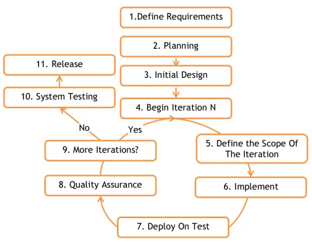
The system development life cycle is a process of creating or altering systems and refers to the models or methodologies that people use to develop those systems (1).The development lifecycle followed the agile methodologies. They were chosen because according to the results of a statistical analysis of a survey made by Scott Amber, the agile methods do indeed improve outcomes from software development projects in term of quality, satisfaction, and productivity, without a significant increase in cost (2). Using a single agile methodology is not always the best choice. The reason is that the development methodologies are designed to be used under certain conditions. When they are changed, it is needed to change the existing model so that it becomes applicable in the new conditions or to combine several different models that work together successfully (3). For the purposes of the project two methodologies were combined: extreme programming and feature driven development. Both of them concentrate heavily on software implementation practices (4), which means that the emphasis was on the application development. In all agile methodologies the software development lifecycle determines the start and the end of the project, essential phases of the project management, the processes and the stages for managing the project (3). This means that the combined process also has the standard stages: gathering user requirements, design and documentation, development, testing and deployment. These phases are illustrated in Figure 2.

(13)

5

The project started with defining the requirements. At the end of this phase, usually most important and time consuming requirements are identified. This allowed creating detailed project planning. Gathering as much as possible requirements at the beginning enable creation of a complete and detailed project plan. This means that only minor changes can be made later at the beginning of an iteration. Thus, the project end date is fairly accurate.

After that an initial design of the application was be created. This includes designing the database and the architecture of the application. Each of these steps was performed once at the beginning of the project. Then the process continued with the realization of the iterations compounding the development stage. The duration of each iteration was in the range of 1 to 3 weeks. An iteration consists of the following phases: implementing the features scheduled for the iteration, testing them and deploying them on a test server. Finally, the

FIGURE 2 SOFTWARE DEVELOPMENT LIFECYCLE OF MYCOURSES PROJECT 1.Define Requirements 2. Planning 4. Begin Iteration N 8. Quality Assurance 11. Release 10. System Testing 6. Implement Functionality 7. Deploy On Test Server

5. Define the Scope Of The Iteration 9. More Iterations?

No _Yes

(14)

6

process ended with a system testing and a deployment. System testing had to verify that the system was developed according to the system requirements. After the system was tested it was released. The phases are explained in details in the next section.

1.2 Process Stages Gathering Requirements

Studies indicate that between 40% and 60% of all defects found in the software projects can be traced back to errors made while gathering requirements (5). Thus, identifying problems during the stage of gathering requirements is vital, because changes are much easier to be made than on a later stage. The reason is that the impact of a later change is much bigger. There are various ways to gather the requirements. Each of them has its advantages and disadvantages, but the most important thing is to use the one that works well for the team. Thus, the methods of feature driven approach were chosen for gathering the MyCourses’ requirements. The advantages they gave in comparison with the extreme programing’s stage are as much as possible requirements are identified in the beginning, UML diagrams are produced and expected final date can be defined. UML diagrams represent the business needs in a way that is understandable for both the customer and the developers. The fact that the features are determined at the beginning of the project, still allows adding features for subsequent releases. This list makes it possible to specify the project’s timeline more precisely in comparison with the XP principles. This means that following FDD a detailed project plan with an approximate completion date can be created.

There are two types of system requirements: functional and non-functional requirements. The functional requirements state what is to perform. This means that they include all requirements associated with implementing the business processes in the system and criteria for their examination (3). While the non-functional requirements specify criteria that can be used to judge the operation of a system, rather than the specific behaviour (6).

(15)

7 Functional Requirements

As mentioned above the approach used in this project is simply keeping a list of requirements borrowed from feature driven development method. They were grouped in logical elements from the business model, for example programs, courses, etc. Once the requirements were collected, a requirements traceability matrix was filled [Table 1, 0, 1.5 Use cases]. For each requirement an identical number, priority and use case name was given. After the features were identified, the use cases were described. Use cases translate the requirements into a package that allows easier understanding of the interaction of a user with the system. Then each use case was described in details as well as the actors. The first two stages of the project life cycle are explained in details in 0.

Non-functional

Non-functional requirements include performance requirements, interface requirements, data requirements, operational requirements, etc. Interface requirements describe interaction of the system with the users. Data requirements describe the data entities, their decomposition and their definitions. They describe the business data needed by the application. They do not describe the physical database and do not identify field names. Operational requirements describe how the system runs and communicates with operations personnel. It defines how reliable the system must be. Both of the types are explained below in the context of the project.

The non-functional requirements defined for the project were data requirements and interface requirements. The interface requirements included building a user friendly interface that allows various users to use the system without difficulty. This included providing a way for users to create and modify a schedule in a simple and fast way. The result is described in 1.16. The data requirements were defined through the entity-relationship diagrams. Thus, the major entities were identified as well as their relationships. They are presented in details in 1.14.

(16)

8 Planning

The next step in the process was defining the planning of the project. Microsoft Project was used for the preparation of the project plan and tracking the progress. The end of each iteration of the incremental process finished with a milestone. Milestones represent the time when a deliverable was ready to be reviewed from the stakeholders. This means each iteration finishes with a complete functionality. While planning, the scheduling algorithm was considered as the most risky task. Therefore, it was scheduled as early as possible in the project plan. An overview of the project plan is shown on the next figure. A complete project plan can be view in Appendix Appendix B.

The project plan was used for tracking the progress during the development. There are several commonly used methods for updating the project plan in the Microsoft Project with the current status. Some of them are using percent complete, actual work and using baselines. The later was chosen. Although this approach gives a more general and a high level view of the completeness status, it is faster and easier to be used. The approach uses the general measures of how complete a task is.

(17)

9 Design and documentation

For this phase the XP principle was chosen, which follows the principle that the coding must be done in a way that the need of documentation is minimized. The reason is because of one of the main principles of agile development process. It states that the working software is more important than an exhaustive documentation. Therefore, too much documentation is worse than too little (3). The documents that were written for the project are the only necessary for developing a working application according to the university needs.

During the phase the data model and the application architecture were designed. This includes identifying the general entities required for the software and their relationships, which are discussed in section 1.14 Database Design. After that the layers were identified described in 0. In addition the algorithm was selected which allowed to verify that the design was appropriate to adopt the algorithm.

Development

The development part of the process was divided into iterations each lasting between 1 and 3 weeks. This phase stacked to XP’s principles, except with the pair programming. XP focuses on the coding stage, minimizing the time spent on other tasks.

Despite the methodology that is chosen, it is essential using source control tool. Subversion was used for this purpose. It is an open source version control system, which requires front end tools. The tools used in MyCourses projects were TortoiseSVN and AnkhSVN. TortoiseSVN is a windows shell extension (7), which requires an additional tool that supports Visual Studio 2010, AnkhSVN. Both of the tools are also open source and are reliable.

The identified bugs with high priority from previous iterations were included in the next iteration following the XP practices. The glitches in the system were managed and prioritized through a bug tracking system named BugNet (8). It is open source software allowing its users to customize the issue’s attributes, flexibility to track issue status and history, etc.

(18)

10

During the development coding standards were followed. This helps the code to be easily read from other people and can be more efficiently reviewed if needed at a later stage. The code convention was a combination of Microsoft’s (9) and Lance Hunt’s convention (10). Another good coding practice that was used is writing good and meaningful comments making the code more maintainable (11). The reason is that the comments tend to become out-dated over the time which usually causes confusion. Such were added in methods with more complicated functionality or in pieces of code with tricky logic.

Testing

Automated tests of the user interface were created using the Visual Studio 2010. It provides a tool called Coded UI Test. The tests created using this tool provides functional testing of the application’s user interface and validation of the user interface controls. Thus, they enable quicker testing of code changes and reduce the risks introducing errors after those code changes. The coded UI test performs actions on the user interface controls for an application and verifies that the correct controls are displayed with the correct values (12). Various tests were recorded focusing on the main business processes in MyCourse’s web system.

Deployment

According to the agile methods the deployment is not executed as the last stage of the process as it is in the waterfall, but also is part of the iteration cycle. The result of each iteration was deployed on a test server as soon as it was completed allowing the completeness of the development to be tracked.

(19)

11

REQUIREMENT ANALISYS

The essence of the requirements was to develop easy to use web-based course scheduler, MyCourses. The web system was built by considering simplicity and the performance of the system. Considering the system was designed for online usage by many different people, its usability and user friendliness is very important. Therefore during the design phase the emphasis was to design a system that will allow users to enter data and requirements in a simple way and calculate an error free schedule.

1.3 Goal

All projects are defined by their goals, objectives, boundaries and constraints. Getting a detailed but clear picture of the project scope will make it possible to complete the project successfully (13). So the first step was to identify the project goal. It has been describes in the task description for this thesis as follows:

The goal of the project is to develop a course scheduler, MyCourses. MyCourses will make it possible to enter data and requirements in a simple way using a web-based interface, calculate and propose a schedule, enable manual updates, and finally present the schedule for the selected courses.

Next thing was to defining the project scope, which included identifying all the work that the project had to accomplish in order to achieve the goal.

1.4 System Scope

The scope of the project was to develop timetable management program that enables entering data, calculates and proposes a scheduling for courses,

(20)

12

allows manual update of a schedule and provides a presentation of scheduled courses. In order to achieve the objectives, the scope of the timetable system covers the following features:

Features Priority

General

1. Reduced gaps for students Should

2. Reduced gaps for lecturers Should

3. Design user interface Must

4. Automatic scheduling programs Must

5. Import/Export students’ data Must

6. Import/Export lecturers’ data Must

7. Import/Export classes’ data Must

8. Import/Export rooms data Must

9. Import/Export programs data Must

10. Online help for different user roles Must 11. Variety of presentations for a program Must

12. List unsatisfied conditions Should

13. Notify users for changes in schedule May

14. Verify schedule for conflicts Must

15. Multi-language user interface Should

Administrator

16. Configure system’s graphic user interface – colour theme and university

logo May

17. Configure different scheduling rules Must

18. Define rooms and details about them Must

19. Login Must

20. Create/Modify lecturers Must

21. Create/Modify students Must

22. Create/Modify other faculty members Must

23.

Allow defining priority of lectures according their type (heads of department, part time lectures, other lecturers, etc.) when scheduling courses

May

Program administrator

24. Define program definition Must

25. Assign program manager Must

26. Import program from previous year Must

Program manager

27. Enter all details about a program Must

28. Enter courses details Must

(21)

13

30. Enter predefinition of a schedule Must

31. Manually make modifications of a proposal Must

32. Freeze schedule Must

Lecturer

33. Define constraints for course schedule he/she is assigned to Must

Main Lecturer

34. Defines the details of courses he or she is assigned to Must 35. Import details of course from previous instance of a course Must 36. Defines requirements for the rooms that the course requires Must 37. Submits a proposal for the courses he/she is assigned to Must

Student

38. View his/her schedule May

TABLE 1 IDENTIFIED SYSTEM FEATURES

In the feature list there are three priority levels defined– must, should and may. Priority “must” is used for the features that are critical for system functioning and must be implemented during the development phase. Priority “should” defines features that are important for the project, but can be omitted for short deadlines. Features with priority “May” are features that would be nice to have.

1.5 Use cases

UML use case diagrams are used to describe the main processes and functionality of the Course Scheduling System. They give a high-level view of the application scenario. The purpose of having use case diagram is to identify the scope of the system. Use case diagrams consist of named pieces of functionality (use cases), the persons or things invoking the functionality (actors), and possibly the elements responsible for implementing the use cases (subjects) (14). Figure 4 illustrates the use cases that exist in the application. The actors on the left hand side are the main actors, e.g. those that will use the system often, and the others are on the right hand side.

(22)

14 Actors

The following actors were identified:

FIGURE 4 MYCOURSES USE CASE DIGRAMS. MAIN ACTORS ARE ON THE LEFT SIDE, WHILST ALL OTHERS ARE ON THE RIGHT SIDE.

(23)

15  Administrator

The administrator is a person who manages and maintains the system. The administrator has full control over the system. The administrator can add, edit and delete new users, assign roles to new and existing users. The administrators can define and edit rooms as well as adding or changing existing room facility types and course types. The administrator is responsible for the system configuration including turning on and off constraints and setting priority for soft constraints, managing timeslots, university periods, school days and holidays.  Program administrator

The program administrator is a user that is responsible for management of the programs at the university. The program administrator identifies the program, its running period (starting and ending year), and a program manager. In cases where no program manager is defined, the program administrator runs the automatic scheduler.

 Program manager

The program manager is a user responsible for a program. The program manager can create a new or modify existing courses, add a course instance to an existing course and assign main lecturer to a course instance. The program manager can run automatic course schedule, manually modify schedule, approve or discard a course proposal from a lecturer, and freeze the schedule.

 Main Lecturer

The main lecturer is a person responsible for details about a course instance he or she is assigned to. Main lecturer can add or modify existing course element for a given course instance. Main lecturer can define the other people that are participating in the teaching process. The main lecturer can copy the data for a course instance from currently existing course instances.

(24)

16

The lecturer is a person who participates in the process of teaching students. The lecturer can see the schedule of courses he or she is teaching.

 Student

The student is a person who attends university courses. The student can view the schedule of courses that he or she is attending.

 System

The system actor is an external system that uses the data that is exported from the application.

Use case description

Use case name: Define programs

Goal: A set of programs for the university is defined Actors: Program Administrator

Preconditions: User should be authenticated Steps:

1. User identifies the program 2. User sets its running period 3. User enters a program manager

Post conditions: A new program is created

Use case name: Import program from previous year

Goal: Program previous year is imported with some changes Actors: Program administrator

Preconditions: User should be authenticated; at least one program from previous years should exists

Steps:

1. User selects a set from programs to import 2. User launches import functionality

(25)

17

Post conditions: A program is imported from previous year

Use case name: Define program specification Goal: All details for the program are entered Actors: Program administrator

Preconditions: User should be authenticated; at least one program should exist Steps:

1. User chooses a program to specify

2. User enters all details for a program - which courses it includes, which courses are obligatory, which courses are optional, etc.

Post conditions: All program details are completely defined

Use case name: Verify schedule Goal: No conflicting constraints Actors: Program manager

Preconditions: User should be authenticated; a schedule should exist Steps:

1. User chooses part of the schedule or the whole schedule 2. User runs verification process

Post conditions: The schedule is verified and no conflicts exist

Use case name: Freeze schedule Goal: A final version of the schedule Actors: Program manager

Preconditions: User is authenticated; all the courses are scheduled without conflicts

Steps:

1. User selects the schedule 2. User marks the schedule as final

(26)

18

Post conditions: The schedule is final and cannot be modified

Use case name: Enter program details Goal: Program details are entered Actors: Program manager

Preconditions: User should be authenticated; Program should exist Steps:

1. User chooses a program to specify

2. User enters all details for a program - which courses it includes, which courses are obligatory, which courses are optional, etc.

Post conditions: Program details are entered

Use case name: Manually update schedule

Goal: A program is updated according to the specific requirement of the user Actors: Program manager; Main lecturer

Preconditions: User should be authenticated; Use should have access to the program

Steps:

1. User selects a program to update 2. User updates the schedule data 3. User saves the changes

Post conditions: A program is updated according to the specific requirement of the user

Use case name: Run schedule Goal: Schedule courses

Actors: Program administrator; Program manager; Main lecturer Preconditions: user should be authenticated

(27)

19 1. User selects a set of courses

2. User launches automatic scheduling

3. User resolve conflicts by updating proposed schedule

Post conditions: The selected courses are scheduled without conflicts

Use case name: Define instance of courses Goal: A new instance of a course is created Actors: Program Manager; Main Lecturer

Preconditions: User should be authenticated; a course should exist Steps:

1. Choose an existing course

2. User creates a new instance of the selected course Post conditions: A new instance of a course is created

Use case name: Mark schedule as proposal Goal: A proposal is defined

Actors: Main Lecturer

Preconditions: User is authenticated; user is assigned to a subject Steps:

1. User selects a course

2. User runs scheduler for the course 3. Use marks the schedule as a proposal

Post conditions: A proposal for a course is defined

Use case name: Add constraints Goal: A constraint is defined Actors: Main Lecturer; Lecturer

Preconditions: User is authenticated; user is assigned to a subject Steps:

(28)

20 1. User selects a course

2. User defines preferences for his or her availability for the course Post conditions: A constraint for lecturer’s availability is defined

Use case name: Define resources Goal: Resources are defined

Actors: Administrator; Program Administrator Preconditions: User is authenticated

Steps:

1. User defines different data about resources Post conditions: Resources are entered

Use case name: View schedule presentation Goal: A presentation of the schedule is visualized

Actors: Administrator; Program Administrator; Program Manager; Main Lecturer; Lecturer; Student

Preconditions: User is authenticated; a schedule is defined Steps:

1. User chooses a program or a set of courses from a program 2. User views the presentation of the selected program Post conditions: A presentation of the schedule is visualized

Use case name: Import/Export Data Goal: Data is transferred

Actors: Administrator; System

Preconditions: user is authenticated; data for export/import should exist Steps:

(29)

21 2. User exports or imports the data

Post conditions: Data is exported or imported in appropriate format

Use case name: Configure

Goal: A scheduling rule are defined Actors: Administrator

Preconditions: user is authenticated Steps:

1. User defines a rule of scheduling

(30)

22

PROBLEM FORMULATION

Before describing the system implementation it is essential to define the problem that it tries to solve. It is separated in two areas. The first one is the actual problem that was solved and the second one is the concrete implementation of the mathematical model.

1.6 Scheduling Problem

University course timetabling problems is an NP-hard problem, which is very difficult to solve by conventional methods and the amount of computation time required to find optimal solution increases exponentially with problem’s size (15). The problem involves assignment of courses to limited timeslots and rooms satisfying a number of constraints. The constraints are divided in two types: hard constraints and soft constraints. Hard constraints are those constraints that must be satisfied when scheduling the timetable. Soft constraints are desirable to be satisfied, but those that are unsatisfied must be kept at minimum. Weights were defined for each constraint allowing prioritization. Hard constraints are more significant than soft constraints. This means that hard constrains have much higher weight, so when they are violated the cost function’s value will be high. The weights of soft constraints might not be equal, which makes some of them more important than others. The following list contains the constraints and the corresponding default weights given in parentheses that were identified during the requirement gathering phase:

Hard constraints:

(31)

23

(H2) No more than one class per room at the same time (1000) (H3) No more than one class per student at the same time (1000)

(H4) Room capacity is less than or equal to course maximum students and facilities required for the course are existing in the room (1000)

Soft constraints:

(S1) Courses are scheduled according to predefined order (100)

(S2) Course elements (lectures, labs, etc.) are allocated according to the lecturer’s preferences (25)

(S3) A course is not scheduled more than a given number of times per week (25)

(S4) The gaps between lecturer’s classes are minimized (10) (S5) The gaps between student’s classes are minimized (10)

A solution satisfying all hard constraints is called feasible solution. If the solution does not violate all soft constraints it is called optimal. The objective is to find a feasible assignment of courses that minimizes the violations on soft constraints. The fact that a weight is given for each constraint, means that a cost function can be defined for evaluating the quality of the solution. This function is an arbitrary measure of the quality of the solution. The optimization problem becomes one of minimising the value of this cost function (15).

1.7 Implementation problems

The above basically defines a representation of the core problem that MyCources project tries to solve, e.g. creating optimal and error free course timetable in fast and easy way. In order for the solver, which is part of the system, to work it needs some data entered and managed through the user interface. Entering and managing the data is done by several user roles: administrator, program administrator, program manager and lecturer. The administrator is responsible for the global settings of the system such as activating and deactivating constraints, prioritizing them, available recourse, etc. Program administrator can manage the programs at the university. He/she

(32)

24

can create and modify existing program details and assign a program manager. The program manager is in charge for program details including the courses that are part of the program and course details. The main lecturer is a type of lecturer with additional rights on a course or a concrete instance of it. The main lecturer can define the details about a course instance and the other lecturers that will participate in the teaching process. The lecturer can specify preferred time for a course part that he/she is in charge of, the time convenient or inconvenient for him/her.

The solver had to implement an appropriate algorithm that handles the university timetabling problem. It has to schedule a course or a set of courses. As a result the courses have to be assigned to a timeslot and a room. In addition the room’s capacity has to be greater or equal the number of students attending the course and has the facilities required for the course. The solver can be run by users from several roles: main lecturer, program manager and program administrator if no program manager is assigned to a program. The main lecturer can schedule his/her courses and mark the output as a schedule proposal. The program manager and the program administrator can run the solver for courses that are part of his/her programs or for a whole program. When schedule is completed and no more changes will be made the program manager can define the program as official, which means that it cannot be modified. This is a brief overview of the use cases that exist. A more detailed explanation is given in section 1.5 Use cases.

MyCourses application had to allow not only specifying which constraints are applied in the university, but also prioritizing the soft constraints. The reason only soft constraints are prioritized is that hard constraints are in high degree physical ones, e.g. it is impossible for a student to attend two classes at the same time, and all of them have to be satisfied. There are some cases when a lecturer can take one or more classes depending on which kind of course he is in charge. In these cases the responsible user should specify whether the teacher is involved in one or more classes at the same time. Thus the necessity of prioritizing and activating constraints required a flexible mechanism for

(33)

25

managing constraints. Moreover new constraints have to be added easily, without breaking the existing code, if required.

An important part of the project was finding a suitable visual presentation of the data appropriate for different user roles. Example of presentations are “Availability and utilization of the facilities”, “Schedule of a particular course”, “Schedule for a faculty member”, “A schedule for a student”, and similar.

(34)

26

ANALYSIS OF THE PROBLEM

1.8 Analogy with Physical Annealing and Simulated Annealing Algorithm Simulated annealing (SA) is motivated by solid state physics: the annealing process. The annealing is a technique involving heating and controlled cooling of a material to increase the size of its crystals and reduce the defects (16). When the solid is heated to a high temperature, its atoms are free to move around allowing them to become unstuck from their original position (a local minimum of the initial energy). The goal is to allow atoms to rearrange while cooling down the solid until they make an ordered configuration. At this state the energy is the lowest which means that it is the state with highest stability. The movements are carried out by random displacements through stages with higher energy. The quality of the result strongly depends on the cooling temperature (17). Slowly cooling down the material makes the atoms to form large crystals and thus the material is free of crystal defects. Whereas, if it is cooled rapidly, the crystals will contain imperfections due to the amorphous structure of the material. This means that this state has a higher energy.

An example of the annealing process is shown in the following figure. The areas with the highest temperature are coloured in red, whereas the coldest parts are coloured in dark blue. The red paths are the cases when the process flowed smoothly, e.g. in each state the system energy is lower than the one in the previous state. The orange curves are the “jumps”. They show the stages in which the energy was higher, but the system configuration was accepted according to the probability from formula (1).

(35)

27 1.9 Simulated Annealing Algorithm

Simulated annealing establishes the connection between this type of thermodynamic behaviour and the search of global minima for a discrete optimization problem (18). The matching of simulated annealing to the physical annealing is relatively straight forward. The atoms are replaced by courses. The energy is replaces by a cost function, change of state by calculating the neighbourhood solution. The cost function reflects the quality of the course schedule, just as the system energy reflects the quality of the material. The temperature controls the probability used for accepting worse solution, such as the temperature in annealing process controls the crystals’ structure.

Simulated Annealing, applied in MyCourses scheduler, starts with a random solution, e.g. each course is assigned to a random room and timeslot. The initial

FIGURE 5 SIMULATED ANNEALING ESCAPING FROM LOCAL MINIMUM BY CHAOTIC JUMPS. (57)

Start

Optimal Solution Start

(36)

28

cost is calculated and the initial temperature is set. Then the algorithm can start to search the optimal solution by moving from one solution to a new one (described below in “Neighbourhood Searching”). On each iteration SA algorithm calculates a new solution from the current one by making small modifications. The new solution is called neighbour. Then the difference (∆) between the cost functions of the current solution and the next solution is calculated. The generated solution is accepted in two cases. The first one is if it does not worsen the overall value of the current solution (19), e.g. ∆ < 0. The second case is when the probability of the increase is lower than the expected at the given temperature T. The probability is calculated using the formula that follows:

( ) ( ) ₍₁₎

Where ∆ is the change of the cost function, T is the current temperature. If this probability is greater than a randomly selected value in the range (0, 1), the new solution is selected. The temperature is decreased by a cooling rate that is between 0 and 1. As the temperature decreases, the probability of accepting worse moves decreases (20). The process continues until the final temperature is reached.

The annealing process stops usually when the temperature reaches 0, but the practice shows that if no progress is made for long time, there is no use of continuing calculating the next solution. There are some implementations that allow the process to terminate after a predefined maximum iteration count is reached.

For easier understanding the following flow chart illustrating the algorithm process is provided.

(37)

29

SA uses random numbers when determine whether to accept a solution or not. This means that the result solution might not be equal every time. That is case when an optimal solution cannot be found, a feasible solution is returned instead.

(38)

30

The design of a good annealing algorithm is nontrivial. It generally comprises three components (21): (1) neighbourhood structure, (2) cost function and (3) cooling schedule.

Neighborhood Searching

SA requires a neighbourhood structure to be defined in order to move from one state to another. The classical simulated annealing swaps two random elements. Unlike it, the neighbourhood in MyCouses’s solver is constructed by unassigning a random course on each iteration. Then the solver tries to assign it to an available timeslot and room. If this is not possible, the course is added to a list of unassigned elements. Then the solver tries to assign a random course from this list which is different from the first one as long as it is possible. On each iteration the solver aims to assign as much as possible courses left unassigned from previous steps. One course can remain unscheduled if no suitable free timeslot and room is available in the current solution. In this way the neighbourhood construction is the closest to the general version of the algorithm. This approach was chosen instead of the original one, where the classes are considered to be with equal duration, two elements are simply swapped. This would cause problems when trying to reschedule classes with different duration.

(39)

31 Cost calculation

As mentioned earlier some of the constraints are more important than other when calculating the timetable. These requirements can be defined by weighting the different components of the cost function. Thus, calculating the cost of a solution means calculating the cost of each constraint. It can be expressed by the following formal formulation. If s is current solution and fi are the individual cost functions for each constraint, where i is between 1 and n. Then the cost function can be calculated with the formula:

Unassging the selected course Other unassigned courses? Select a random course Stop Select unused unassging course Can assign it?

Assign the course Yes

Yes

No

(40)

32

( ) ∑ ( )

(2)

where n is the number of constraints.

In the general case the computation of the cost function is the most expensive part of the algorithm. Instead of calculating every time the cost function of the timetable, it can be improved by evaluating the cost of the difference. This means that the cost of unassigning a course from a period is subtracted from the cost of assigning it to another period (22).

Cooling rate

Cooling rate is an important part of the Simulated Annealing algorithm as it determines the effect of the cooling process, e.g. the quality of the solution. According to a number of experiments conducted by D. Abramson in (23), the optimal cooling rate is determined. During the test the same input values were annealed using different control parameters. The cooling rate values studied were 0.1, 0.5, 0.9, 0.95 and 0.99. According to the results increasing the cooling rate (i.e. slower cooling) produces better results (23). One possible explanation of the result is that very slow cooling allows exploring large portions of the search space. Thus, the algorithm gets stable cost of the final solution. The results of several researches ( (24), (25), (23), (26), (27)) including the mentioned above suggest that the cooling rate should be between 0.80 and 0.99. The cooling rate for MyCourses was fixed at 0.99.

1.10 Implementation of Simulated Annealing

As a conclusion of the structure of Simulated Annealing algorithm explained above, a pseudo code is presented to provide more thorough understanding. It outlines the main steps which the implementation of the algorithm follows while searching for a solution. The pseudo code is presented in Figure 8.

(41)

33

The function SimulatedAnnealing takes three input parameters. The parameter initial that contains the initial solution, initialTemp is the initial temperature the algorithm starts from and finalTemp is the final temperature that the algorithm has to reach. The function returns the best solution found by the algorithm.

FIGURE 8 PSEUDO-CODE OF SIMULATED ANNEALING

function SimulatedAnnealing(initial, initialTemp, finalTemp) {

current = initial; best = current;

//Set current temperature to initial temperature

Temp = initialTemp;

//Set decreasing temperature rate

tempRate = (log (initialTemp) - log (finalTemp))/IN; while (Temp > finalTemp)

{

//Generate new solution (solutionNew) by Applying //Random neighbourhood from different neighbourhood //structure to the current solution “current”

//Calculate Fitness (solutionNew);

if (Fitness (solutionNew) < Fitness (best)) { current = solutionNew; best = solutionNew; } else {

delta = cost(solutionNew) - cost(current) randomNumber = GenerateRandNumber(); if (randomNumber ≤ e - delta/Temp )

current = solutionNew; }

Temp = Temp - Temp * tempRate; }

return best; }

(42)

34

TECHNOLOGIES

This section outlines the technologies used for the development of MyCourses project. Because the timetabling system is a web-based system, the client-server model is applied. The client-server describes the relationship between two computer programs in which one program, the client, makes a service request from another program, the server, which fulfils the request. This requires the usage of two types of technologies - server-side technologies and client-side technologies, which are outlined in the sections below.

1.11 Server-side Technologies

Server-side technologies, commonly used in e-commerce applications and back-end databases, provide interactive web sites that allow a user to interface databases and retrieve or modify data residing on a web server (28).

1.11.1. .Net Platform

.Net is a software platform. It is a collection of tools, technologies, and languages that all work together in a framework to provide solutions that are needed to easily build and deploy truly robust enterprise applications. These .NET applications are also able to easily communicate with one another and provide information and application logic (29).It is a language-neutral environment for writing programs that can easily and securely interoperate. The .Net platform encapsulates four technologies and ideology components: .Net Enterprise Servers, .Net Framework and Visual Studio, Building Block Services, and .Net Smart Clients (30). For the development purposes of the project the following parts of the .net were used:

(43)

35

1.11.1.1. .Net Framework

.Net Framework is a software platform for development and execution of .Net products. It gives programming model and a base class library for application development and unified environment for execution of managed code. It supports different programming languages and their collaboration. The .NET Framework provides tools and solutions for building rich applications in the stateless environment of the Internet.

The following figure shows the .Net 4.0 Framework architecture. The .Net Framework consists of two main components – the common language runtime and the base class library. Each of these parts plays an important role in the development of .NET applications and services.

(44)

36

FIGURE 10 .NET FRAMEWORK 4.0

Common Language Runtime (CLR) is the foundation of the .Net Framework. It is a virtual machine that manages the execution of the .Net code. It provides various services such as memory management, thread management and other system services. CLR also enforces type control and code accuracy. It allows programs written in any of the supported languages, to share common object-oriented classes. The programmers need not to worry about managing the memory themselves in the code. Instead CLR will take care of that letting the programmers to focus on the logic of the application.

The second core component of .Net Framework is the class library, which is divided in two parts – the Framework Class Library (FCL) and the Base Class Library (BCL). The Framework Class Library is a collection of thousands of

(45)

37

reusable classes, interfaces and value types (31). The Base Class Library (BCL) is part of the FCL that provides the most fundamental functionality. BCL is comprehensive object-oriented collection of reusable types and classes that provides base system functionality. BCL enables developers to accomplish a wide range of common programming tasks, such as input-output operations, data collection, string management, network services, security, multithreading and others.

The top layer of the .Net framework architecture is the layer for building interface for the end user of the application and provides functionality for web and windows based user interface as well as web services. ASP.NET provides an easier way for building dynamic web sites and web applications and web services.

ASP.NET

ASP.NET is a web application framework marketed by Microsoft that programmers can use to build dynamic web sites, web applications and XML web services. It compounds the interface layer to the end user of the application and provides rich functionality for creating web-based user interface. ASP.NET gives an easy way for developing flexible dynamic web sites and applications. It can be used to create anything from small, personal websites to large, enterprise-class web applications. ASP.NET aims for performance benefits over other script-based technologies by compiling the server-side code. ASP.NET pages execute on the server and generate markup such as HTML, WML, or XML that is sent to the browser. ASP.NET pages use a compiled, event-driven programming model that improves performance and enables separation of application logic and user interface (32).

ADO.NET

ADO.NET provides consistent access to data sources such as Microsoft SQL Server, as well as data sources exposed through OLE DB and XML. Data sharing

(46)

38

consumer applications can use ADO.NET to connect to these data sources and retrieve, manipulate and update data.

LINQ to SQL

LINQ stands for Language INtegrated Query. It was introduced in .Net Framework 3.5. It gives query capabilities using C# and Visual Basic. Visual Studio 2008 and higher comes with LINQ provider assemblies with capabilities of querying in memory collections, SQL relational database, ADO.NET datasets, XML documents and other data sources (Figure 11 shows the LINQ architecture) (33). LINQ is actually a set of operators, called standard query operators, which allow the querying of any .NET sequence. The queries are integrated into the language which allows they are verified compile time and there is a design time support.

LINQ is based on one of the new features introduced in .NET Framework 3.5, lazy evaluation. Lazy evaluation is essential for performance of LINQ queries, because it avoids generation of intermediary unnecessary results by delaying the execution until the latest possible moment, when all information about what is wanted is known.

LINQ to SQL is a dialect of LINQ that allows the querying of a SQL Server database. It also includes object relational mapping and tools for generating

FIGURE 11 LINQ ARCHITECTURE (33) Data Sources

.NET Languages supporting LINQ Language Integrated Query ADO.NET LINQ to Datasets LINQ to SQL LINQ to Entities LINQ to Objects LINQ to XML

(47)

39

domain model classes from a database schema (34). Rather than mapping to a conceptual data model, these generated classes map directly to database tables, views, stored procedures and user-defined functions. Entity partial classes are generated for each table that map the database. Each entity has properties corresponding to the table columns. Instances of so created entity classes can be used as data transfer objects (or also called Data Mapper by Martin Fowler (35)).

DataContext

The data context is the source of all entities mapped over a database connection. LINQ to SQL queries are converted using the DataContext into native SQL queries. DataContext provides the ability to manipulate SQL data through the entity classes. It tracks changes that the developer makes to all retrieved entities and maintains an “identity cache” that guarantees that entities retrieved more than one time are represented by using the same object instance (36).

At the same time the DataContext implements a number of other commonly used patters for a domain model:

- identity map pattern is applied when DataContext is cashing copies of all objects retrieved from the database during an operation. As long as the DataContext instance is alive, the same copy of the object is returned without the need of a new query.

- lazy loading pattern allows only a specific part of the model’s graph to be loaded.

- optimistic offline lock pattern is applied when DataContext ensures that any changes that are about to save are not conflicting with changes that another transaction may have committed.

- unit of work pattern is applied when DataContext tracks changes made to any object that is loaded. At any time the DataContext knows

exactly what changes and how (delete, update, insert) has occurred. This knowledge makes possible to submit all pending changes in transaction.

(48)

40

- data mapper pattern is the abstraction that represents the mapping between the SQL Server database and the auto-generated domain objects.

T4 Templates

T4 Templates (Text Template Transformation Toolkit) is a template-based powerful code generation engine shipped out of the box within Visual Studio. It can generate C#, Visual Basic, T-SQL, XML and any other text files. The text templates consist of text blocks and control logic that can generate a text file (37). Text templates can be used for code generation and runtime text generation. The runtime text generation can be used to generate part out the program output, for example HTML report, while the code generation generates part of the source code that is used in the application. Only code generation capabilities have been used in MyCourses project.

The only thing that is needed to make it generate code is simply adding a T4 Template with the extension “tt” and Visual Studio will do the rest. The T4 engine performs two steps to generate the template output. During the first step it parses the processing instructions, text and code blocks, generates a concrete TextTransformation class, and compiles it into a .Net assembly. During the second step, the T4 engine creates an instance of the GeneratedTextTransformation class, calls it TranformText method and saves the string it returns to the output file (38). The example output file bellow (Figure 12) contains the generated source code for MyClass class.

The following is a simple example illustrates how to generate “Hello World” method in class with a given name using T4 template (39).

(49)

41

This template will generate a class with the name specified in ClassName

field. When the template is saved the following class is generated: FIGURE 12 T4 TEMPLATE THAT GENERATES CLASS WITH NAME

SPECIFIED IN FIELD CLASSNAME.

FIGURE 13 GENERATED CLASS WHEN THE ABOVE T4 TEMPLATE IS SAVED.

<#@ template language=“C#” #> // <autogenerated>

// This code was generated by a tool. Any changes made manually will be lost

// the next time this code is regenerated. // </autogenerated>

using System;

public class <#= this.ClassName #> {

public static void HelloWorld() {

Console.WriteLine(”Hello, World!”); }

} <#+

string ClassName = “MyClass”; #>

// <autogenerated>

// This code was generated by a tool. Any changes made manually will be lost

// the next time this code is regenerated. // </autogenerated>

using System;

public class MyClass {

public static void HelloWorld() {

Console.WriteLine(“Hello, World!”); }

(50)

42 1.11.1.2. Microsoft SQL Server

Microsoft SQL Server is a Relational Database Management System (RDBMS) designed to run on various platforms ranging from laptops to large multiprocessor servers. It is commonly used as a backend system for websites and corporate systems and can support thousands of concurrent users. Microsoft SQL Server is comprehensive, integrated data management and analysis software that enables organizations to reliably manage information and confidently run today’s increasingly complex business applications.

1.12 Client-side Technologies

Client-side technologies give the user a nice representation of the data that is manipulated and stored from server-side technologies.

XHTML

XHTML stands for eXtensive Hyper Text Markup Language. XHTML is a markup language designed to structure information for presentation of web pages. XHTML is used to create hypertext documents that are platform independent. XHTML is the same as HTML, except it has clearer syntax. It uses the same tags as HTML, but it adds some new rules, such as each opening tag needs to have corresponding closing tag; tags need to be nested properly; tags must be in lowercase; all attribute values must be quoted and there must be only one root element.

It is preferable to use XHTML than plain HTML if the website is an e-commerce site, it accesses a database or another source of information that uses a different programming language. It is also preferred if the web site is expected to grow and exist for many years.

XHTML is used to be compatible with XML programming. Following the rules would make it possible to include XML programming in the future. For example, XHTML is used when referring to XML files used for RSS feeds, some music players and many more applications (40).

(51)

43 Cascading Style Sheets (CSS)

Cascading style sheets control the way web pages are displayed in the browser, and allow the separation of presentation from structure and content. CSS helps to ensure that the web pages are presented in an accessible way to all visitors over a range of different browsers.

JavaScript

JavaScript is a lightweight scripting technology which is used alongside XHTML documents to make websites more interactive. JavaScript allows developers to make the static web pages interact with the users and react on

FIGURE 14 SAMPLE HTML DOCUMENT.

FIGURE 15 SAMPLE STYLE FOR BODY ELEMENT.

<!DOCTYPE html PUBLIC

"-//W3C//DTD XHTML 1.0 Transitional//EN" "http://www.w3.org/TR/xht ml1/DTD/xhtml1-transitional.dtd">

<title>MyCourses - Home</title> </head> <body> <p>Welcome to MyCourses</p> </body> </html> body {

background: #FFFFFF url(../images/img04.gif) repeat-x;

font-family: "Trebuchet MS", Arial, Helvetica, sans-serif;

font-size: 13px;

margin: 0;

padding: 0;

color: #7F7772; }