Do the Stock Market and the Commercial Real Estate Market Cointegrate? : A Study for Sweden

Do the Stock Market and the Commercial

Real Estate Market Cointegrate?

A Study for Sweden

Master’s thesis within Business Administration and Finance Authors: Annika Florin 901019

Evelina Magito 910531

Tutors: Prof. Andreas Stephan PhD Candidate Jan Weiss Examiner: Assistant Prof. Urban Österlund Presentation: May 22nd _{2014 at 08.00}

Acknowledgements

We would like to thank our supervisor Andreas Stephan for his support and guidance throughout the thesis process. We would also like to thank the assisting supervisors for their feedback during the seminars. Lastly, we would like to thank the other students attending the same seminars for providing us with helpful feedback. Your guidance and support are very appreciated by us.

X

Annika Florin

X

Evelina Magito

Jönköping International Business School Sweden, May 2014

Civilekonom Examensarbete Företagsekonomi (30hp)

Title: Do the Stock Market and the Commercial Real Estate Market Cointegrate? – A Study for Sweden

Author: Annika Florin and Evelina Magito Tutor: Andreas Stephan and Jan Weiss Date: May 2014

Subject terms: Cointegration, causality, correlation, commercial real estate market, stock market, diversification

_____________________________________________________________________

Abstract

In recent years, investors have become more concerned about where they invest their capital and how to spread the risk among different asset types. The interest in commercial real estates has increased as this market is seen as less volatile than the stock market. Previous research for other economies has found that the commercial real estate market and the stock market do not cointegrate. Therefore it is possible to invest in both asset classes to create diversified portfolios. This thesis examines if such cointegration relationship exist on the Swedish market. Furthermore, the thesis examines the correlation and the lead-lag relationship between the two asset classes. The observed data is quarterly between the years 1994-2013 and the indices used are OMX Stockholm, sold multi-dwelling and commercial buildings, and sold manufacturers industries. To examine if there exist any cointegration between the indices the Engle-Granger 2-step method is used and the lead-lag relationship is tested by using the Granger Causality test.

The results from the different tests do not show any short- or long-term relationship between the Swedish stock market and the Swedish commercial real estate market, neither do the assets show any lead-lag relationship. This means that the portfolio risk decreases and it is therefore possible for investors to diversify their portfolios with both short- and long-term time horizons.

Table of Contents

1

Introduction ... 1

2

Frame of Reference ... 6

2.1 The History of the Swedish Commercial Real Estate Market and the Stock Market... 6

2.1.1 The Swedish Commercial Real Estate Market ... 6

2.1.2 The Swedish Stock Market ... 7

2.2 Previous Research ... 9

2.3 Relationship between Real Estates and Stock Returns... 13

2.4 Modern Portfolio Theory ... 14

2.4.1 Portfolio Risk ... 15

2.4.2 Minimum Variance Portfolio ... 16

2.4.3 Risk Preferences ... 17

2.4.4 Sharpe Ratio ... 17

2.5 Investment Alternatives ... 18

2.5.1 Characteristics of a Direct Real Estate Investment... 18

2.5.2 Investment Alternatives in Real Estates ... 19

2.5.3 Investment Alternatives on the Stock Market ... 20

3

Method ... 22

3.1 Research Methodology ... 22

3.2 Data ... 22

3.2.1 OMX Stockholm... 23

3.2.2 Sold Multi-dwelling and Commercial Buildings ... 23

3.2.3 Sold Manufacturers Industries ... 24

3.2.4 Discussion of Data... 24

3.3 Cointegration ... 24

3.3.1 Stationarity ... 25

3.3.2 The Engle-Granger 2-step Method ... 27

3.4 Correlation and Standard Deviation... 28

3.5 Test for Lead-lag Relationship ... 29

3.6 Discussion of Methods ... 29

4

Empirical Results and Analysis ... 31

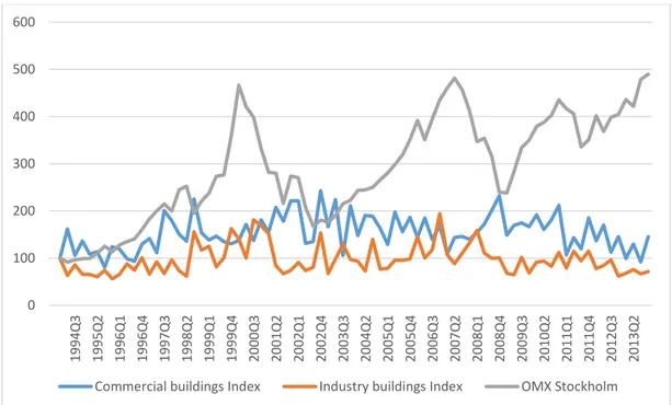
4.1 Historical Data ... 31

4.2 Test for a Unit Root ... 32

4.2.1 Test for a Unit Root in the Commercial Buildings ... 32

4.2.2 Test for a Unit Root in the Industry Buildings ... 33

4.2.3 Test for a Unit Root in OMX Stockholm ... 34

4.3 Engle-Granger 2-step Cointegration Test ... 35

4.4 Lead-lag Relationship ... 36

4.5.1 Correlation ... 37

4.5.2 Standard Deviation ... 38

4.5.3 Evaluation of the Portfolio ... 40

4.6 Integrated Analysis ... 41

5

Concluding Remarks ... 44

6

References ... 47

7

Appendices ... 50

7.1 Appendix 1-4 Unit Root Test for Commercial Buildings ... 50

7.2 Appendix 5-6 Unit Root Test for Industry Buildings ... 53

7.3 Appendix 7-10 Unit Root Test for OMX Stockholm ... 54

7.4 Appendix 11-14 Unit Root Tests for the Residuals ... 57

7.5 Appendix 15: Granger Causality Test ... 60

List of Figures

Figure 2.1: Efficient frontier for portfolios with multiple assets... 15

Figure 4.1: Nominal price movements with 1994Q1 as base ... 31

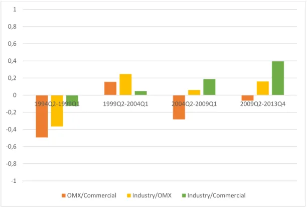
Figure 4.2: Correlations over five year periods... 38

Figure 4.3: Minimum Variance Portfolio ... 40

List of Tables

Table 4.1: Unit root tests for the levels on commercial buildings ... 33

Table 4.2: Unit root tests for the first difference on commercial buildings ... 33

Table 4.3: Unit root tests for the levels on industry buildings ... 33

Table 4.4: Unit root tests for the levels on OMX Stockholm ... 34

Table 4.5: Unit root tests for the first difference on OMX Stockholm ... 34

Table 4.6: Unit root test on the residuals with OMX Stockholm as the dependent variable ... 35

Table 4.7: Unit root test on the residuals with commercial buildings as the dependent variable ... 35

Table 4.8: Granger Causality test ... 36

Table 4.9: Correlations over the period 1994Q2-2013Q4 ... 37

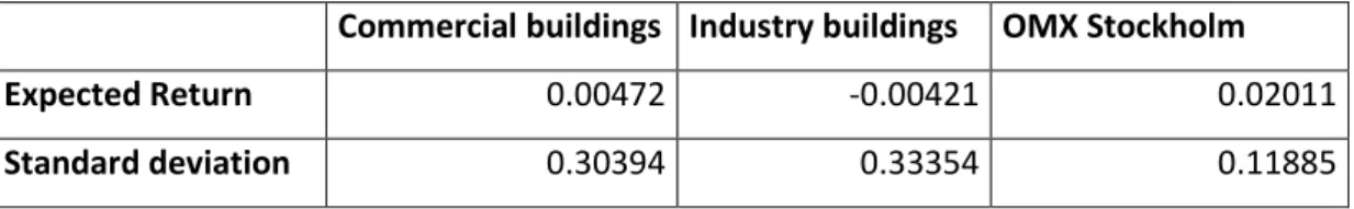
Table 4.10: Risk and return per quarter over the whole observation period ... 39

Table 4.11: Total annual return in percentage ... 39

Definitions

Commercial real estate: Investments in commercial real estates are used for business purposes. This type of real estates includes office buildings, retail premises, warehouse storages and industries.

Cointegration: Cointegration measures the long-run relationship between two variables.

Segmentation: Two variables are segmented if they do not cointegrate.

Short-run: The short-run time horizon in this thesis is zero to two years.

Long-run: The long-run time horizon in this thesis is more than two years.

1 Introduction

In this chapter we introduce the reader to cointegration analysis and how it can be used to forecast a possible long-run relationship between the stock market and the commercial real estate market. This chapter also includes a problem discussion followed by purpose and research questions.

1.1 Background

The study of cointegration between the stock market and the real estate market is important to both institutional and private investors. Stocks are relatively convenient assets to invest in since they usually are both liquid and have low transaction costs, whereas an investment of a real estate is often a more important decision, given that it is a more expensive and more illiquid asset (Lin & Lin, 2011). Despite that, a real estate can be a good asset to invest in because it usually has lower price fluctuations compared to the stock market (Fraser, Leishman, & Tarbert, 2002).

This thesis studies the cointegration between the stock market and the commercial real estate market. Cointegration measures the long-run relationship between two variables. In the literature, there are different opinions if such cointegration exists. A number of authors (e.g. Liu, Hartzell, Greig, & Grissom, 1990; Wilson, Okuen, & Ta, 1996) argue that the returns from commercial real estate do not appear to be highly cointegrated with the stock market, while other studies (e.g. Ling & Naranjo, 1999) find evidence on cointegration. If these two markets are cointegrated the investor could use this information to predict one market by observing the other market. On the other hand, if the markets are segmented it could provide investors with great diversification benefits (Lin & Lin, 2011). By creating a multi-asset portfolio with segmented assets the investor will be able to reduce some of the portfolio risk (Fraser, Leishman, & Tarbert, 2002).

The number of studies that have found evidence of segmentation between the markets are somewhat surprising since both markets are affected by the same factors, such as economic activity and interest rates (Quan & Titman, 1999). A decrease in interest rate

tends to increase asset returns, whereas an increase will have the opposite effect. However, this correlation can be reduced by other factors, such as rental growth, booms and busts. The trends in rental growth are one of the main factors that drives the commercial real estate returns. It follows economic activity when it peaks but as the economic activity decreases the rental growth tend to lag. Booms and busts tend to increase the risk of commercial real estate investments but since the performance of the commercial real estate market have shown evidence to be lagged in the economic cycle, this tend to reduce the correlation with the stock market (Fraser, Leishman, & Tarbert, 2002).

The study of volatility on the stock market is much more extensive than the study of fluctuations on the commercial real estate market (Wilson, Okuen, & Ta, 1996). As institutional investors have become more active in the purchase of commercial real estates, this market has shown a tendency of price fluctuations (Quan & Titman, 1999). However, as commercial real estates are of a non-liquid nature it makes the market inefficient compared to the stock market, which in turn tend to lag and smooth out prices and returns (Fraser, Leishman, & Tarbert, 2002).

Previous research on the cointegration between the stock market and the commercial real estate market has been done for different countries, such as U.S., U.K., Australia and Singapore. However, to the best knowledge of the authors, a recent study of this kind has not been performed on the Swedish market, which makes it an interesting market to study. Furthermore, the Swedish market is interesting to study as it did not experience any major problems on the commercial real estate market during the recent financial crisis, which most of the other countries did (Nordlund & Lundström, 2011). Since the stock market decreased during this crisis and the commercial real estate market did not, this could be an indication that there do not exist any relationship between these two markets.

1.2 Problem Discussion

Diversification is a well-known technique to reduce portfolio risk. It is common for investors to diversify their portfolios within the same class of assets, but an even better approach to reduce risk is to diversify among different assets classes, thus creating a

multi-asset portfolio. Common assets to invest in are stocks and bonds. With this thesis, we intend to examine if it is possible to create a well-diversified portfolio by combining OMX Stockholm with commercial buildings and industrial buildings.

As investors have different time horizons for their investments it is essential to be aware of both the short- and the long-term relationship between the two markets. Correlation tests are used to test for the short-run relationship whereas cointegration tests measures the co-movement of the markets and thus test the long-run relationship. If the markets have a high degree of correlation and cointegration the diversification benefits are poor, hence, commercial real estates securities are not a good complement to get a diversified portfolio. However, this result could instead help to predict the future of one market by observing the other market. On the other hand, if there are no sign of correlation and/or cointegration it could offer investors great diversification benefits.

Investors have different risk preferences. Some are risk averse while others are risk seekers. With this in mind, it is important to get the knowledge of how risky an asset is. This can be measured with volatility. As the investor takes on more risk, the possibilities of generating higher returns are greater. By measuring volatility and return on the commercial real estate market and the stock market it is possible to observe if the market with the highest volatility also have the highest return.

1.3 Purpose

The purpose of this thesis is to examine if there exist any short- and/or long-term relationship between the Swedish stock market and the Swedish commercial real estate market. Further, we examine the volatility of the markets to observe if the market with the highest volatility also has the highest return. By considering both the relationship and the volatility we will be able to create better diversified portfolios for institutional investors with different risk preferences and time horizons.

1.4 Research Questions

With this thesis we want to examine and answer the following questions:

 Are there any short- and/or long-term relationship between the Swedish stock market and the Swedish commercial real estate market?

o How can these results be used when creating a portfolio?

 Which market has the highest volatility and return?

o How will this affect the percentage part of each asset included in a portfolio?

o Does the market with the highest volatility have the highest return?  If no, what are the reasons for this?

1.5 Academic Contribution

This thesis contributes with new knowledge on how the Swedish stock market and the Swedish commercial real estate market relate to each other. Previous research of this type has been performed on other markets, such as the U.K., the U.S. and the Asian markets, but it has not been performed on the Swedish market. Many of the previous studies have performed cointegration tests on these assets, whereas in this thesis we also include tests for correlation and lead-lag relationship which tests the short-run relationship. By performing several tests it provides us with a better overall picture and also with a more robust result. Furthermore, we create different portfolio alternatives that are suitable for investors with different risk preferences.

1.6 Delimitations

This thesis focus on whether there exist any relationship between the Swedish commercial real estate market and the Swedish stock market rather than discussing the underlying macroeconomic factors that affects the returns on the markets. These factors will therefore not be taking into account.

Furthermore, the focus will be on commercial real estates and will not include residential real estates. Therefore this thesis will not focus on individual investors as

they are unlikely to invest in the commercial real estate market. This since commercial real estates are very expensive and it is difficult for these investors to diversify portfolios consisting of commercial real estates.

We will not observe specific geographical areas as the data studied covers the whole Swedish commercial real estate market. Furthermore, the commercial real estate indices only cover the appreciation of the commercial real estates and not the current earnings, such as rental prices. Since there are some flaws with the data, the results in this thesis may only claim if there exist any relationship between the stock market and the commercial real estate market. Further research is needed to ensure this relationship. Years before 1994 will not be considered because data availability is rather limited for years before 1994. Further, regarding interpretation of the result, we believe that the years between 1994 and 2013 are sufficient enough.

2 Frame of Reference

This chapter presents the history of the commercial real estate market and the stock market and is followed by the previous research on cointegration analysis. In this chapter we also present different investment alternatives and the modern portfolio theory.

2.1 The History of the Swedish Commercial Real Estate

Market and the Stock Market

By studying the history of the stock market and the commercial real estate market it provides us with an overall picture of how these markets have performed in previous years. It also provides us with an insight of the factors that affect the Swedish markets.

2.1.1 The Swedish Commercial Real Estate Market

In the 1970s and 1980s the Swedish commercial real estate sector was in a growing stage, with an increased demand for commercial real estates. The ownership structure of commercial real estates were changed and got a more financial structure, which made the commercial real estate market more liquid (Nordlund & Lundström, 2011).

In the first period of the 1980s there were poor conditions for the economy. The real interest rates were high, which was due to low inflation rates. During the second half of the 1980s the economy showed an improvement in the conditions. The real interest rates declined, which was reflected by an increase in asset price inflation. Together with other factors, such as financial deregulation, this led the real estate bubble to burst. According to professor Jaffee (1994) this is one of the major reasons for the crisis to occur. The Swedish economy suffered severe from the crisis, with high loan default rates, decrease in asset prices, negative financial situation for the lending institutions and high vacancy rates. This in turn led to huge losses for the investors of the commercial real estates but also for the major banks as the investors were not able to repay their debts. The crisis had a major impact on all kinds of commercial real estates, but the office buildings in the cities were affected the most (Jaffee, 1994).

The 1990s were marked by poor conditions for the Swedish economy, with an increase in real interest rates, reduction of the housing sector subsidies and falling real estate prices. Not until the middle of the 1990s the Swedish economy started to recover from the severe crisis (Jaffee, 1994).

The prices for the commercial real estates are primarily determined by the rental prices but also by the returns from investors’ investments. After the crisis in the 1990s, the prices for the commercial real estates have followed the development of the rental prices. There has only been one deviation in 2005-2007, where the prices of the commercial real estate rose dramatically compared to the rents. During 2007 the prices of the commercial real estates increased with 14% in Stockholm and 20% in Göteborg, while the rental prices and the demand for commercial real estates were almost unchanged (Nyberg, 2007). The ownership structure of commercial real estates, which was changed during the 1980s, was changed after the crisis in the 1990s as it got involved in the global market (Nordlund & Lundström, 2011). Since then, the Swedish commercial real estate market has been more attractive for foreign countries and, in 2006, 40% of the investments in this market were made by foreign investors. This has had a positive effect on the Swedish market as the risk has been diversified and the Swedish commercial real estate market has become more liquid (Nyberg, 2007).

Recently the interest for investing in commercial real estates has increased. This has especially been observed during the financial crisis as the commercial real estate market is seen as less volatile than the stock market. Though, as the banks are rather cautious with lending money to investors it is quite difficult for small investment companies to acquire commercial real estates to their portfolios as they do not have alternative financial opportunities (NAI Svefa, 2013).

2.1.2 The Swedish Stock Market

In the early 1980s the credit regulations in Sweden were rather strict. This affected the stock market as it limited the choices of portfolios and also the tax-arbitrage transactions. Due to a rapid development of the financial markets, there was a deregulation of the Swedish economy in the middle of the 1980s. This led the stock market index to raise dramatically and between the years 1985 and 1988 the index

increased by 118%. Though, the years before the deregulation, between 1982 and 1985, the stock market index rose with 97%, which could have been an indication of a long-term trend. The deregulation had positive effects on the market as it increased the competition on the credit markets and also over the market shares (Englund, 1999). The 19th of October 1987 the Black Monday occurred, the day where the Dow Jones decreased with 22.6%. At the beginning, the Swedish stock market was not as affected as it only fell 6% that day and 8% the day after. Though, after a couple of weeks the index fell about 40%. According to the economist Claes Hemberg, from Avanza, the decrease in 1987 was not as disastrous for the Swedish stock market as it was to the rest of the world (SvD näringsliv, 2012). For the Swedish stock market, the Black Monday was just an indication of what was coming in the next years; the financial crisis (Bernhardsson, 1996). On the 16th of August 1989 the stock market index had its peak. After that day the stock market index started to drop and in one year it fell with 25%, while the commercial real estate index fell with 52% that year (Englund, 1999). In 2008 the world economy was hit by another financial crisis and the Swedish stock market index fell with 42% (SvD näringsliv, 2009).

During the past decades the stock market has shown a tendency of being rather volatile and due to an unstable international financial market this has led to an increased interest in alternative investments, such as direct investments in commercial real estates. Historically it has shown that downswings in the stock market have increased the direct investments of commercial real estates. After the crisis in 2008 until 2012 the return from the stock market have increased with 14.4% compared to the return of 9.6% for the commercial real estates (NAI Svefa, 2011).

In 2012 the total value of all the shares listed on Stockholm stock exchange were about 3.9 billion SEK, which was an increase of 12% from 2011. Throughout the years more investors from other countries have shown their interest in the Swedish market and, in 2012, 40% of the investments in the stock market were made by foreign investors (Sveriges Riksbank, 2013).

2.2

Previous Research

In portfolio management, the relationship between different assets is important to understand for efficient allocation because investors want to maximize the returns of their portfolios (Lin & Lin, 2011). During the last three decades institutional investors have changed their approach of investing by becoming more active in the direct purchase of commercial real estates. This may have been motivated by academic studies which propose that the covariance between the stock market and the commercial real estate in the U.S. are rather low (Quan & Titman, 1999).

One of the primary studies that investigated to which extent the commercial real estate market and the capital market are segmented was done by Liu, Hartzell, Greig, & Grissom (1990). They define integration and segmentation as follows:

“Integration exists if the only risk that is priced for both real estate and stocks is

the systematic risk relative to the overall market index. No additional premium is therefore associated with real estate market risk. Investors thus earn the same risk-adjusted expected return on stocks and commercial real estate.

Segmentation arises if the only risk that is priced for real estate is systematic risk relative to the commercial real estate market. Investors, therefore, do not necessarily earn the same expected return on commercial real estate and stocks.” (Liu, Hartzell, Greig, & Grissom, 1990, pp. 261-262)

By using a single-factor Capital Asset Pricing Model (CAPM) developed by Jorion and Schwartz (1986) they reach the conclusion that the commercial real estate market is segmented from the stock market in the U.S. market when appraisal-based returns are used. However, they find conflicting evidence that the commercial real estate market is integrated with the stock market when equity real estate investment trusts (REIT) was used for testing (Liu, Hartzell, Greig, & Grissom, 1990). Similar studies were conducted by Wilson, Okunev, & Ta (1996), Okunev & Wilson (1997), Ling & Naranjo (1999) and Liow (2006) but the results has to some extent been differing.

Wilson et al. (1996) used the Arbitrage Pricing Model (APM) to test if the real estate and the stock market on the Australian market were cointegrated. They found that the cointegrated relationship was weak between these two assets.

Another approach on the study of cointegrating relationship between the stock market and the real estate market was conducted by Okunev & Wilson (1997) when they discussed that the cointegration between the two markets may not be linear. They came up with a nonlinear test which allowed for a stochastic trend term. The results of the test showed that the markets are fractionally integrated. This was compared to the result of an established Engle-Granger cointegration test which suggested that the real estate and the stock markets are segmented. The results from this study differ substantially from previous studies, as they found that the two markets fractionally integrate.

Ling & Naranjo (1999) used the multifactor asset pricing model to test for integration between both the exchange traded, the non-exchange traded commercial real estate market and the stock market on the U.S. market. Their results supported their hypothesis that the exchange traded real estate market, including REITs, are integrated with the stock market. They also found that when smoothed out real estate returns were used for testing, the integration was rejected. This is consistent with the results from Liu et al. (1990).

Liow (2006) investigated the long- and short-run relationship between the stock market and the real estate market on the Singapore market by using an Autoregressive Distributed Lag (ARDL) cointegrating model. They found a long-run relationship between the two markets. However, both the long-run and the short-run relationship decreased after controlling for macroeconomic variables.

From an international perspective, Quan & Titman (1997), examined the relationship between the stock market and the real estate market in 17 countries. Consistent with previous studies they found that there is no significant relationship between the two markets in the U.S. However, for the United Kingdom, Japan and some other smaller countries they found a strong positive relationship between the stock market and the commercial real estate market. Furthermore, they found that if economic activities affect corporate profits and rents at the same time it may cause the stock market and real estate market to move together. Rational and irrational expectations of future profits and rents also tend to increase the relationship between the two markets.

In addition to the study of cointegration between the stock market and the real estate market, the causality relationship could help to explain to which extent the two markets

are causally related. Okunev, Wilson, & Zurbruegg (2000) studied the dynamic relationship between the real estate market in the U.S. and S&P 500 index by employing both linear and nonlinear causality tests. The result from the linear causality test were spurious, which means that causality runs from the stock market to the real estate market even though there is no evidence of any long-run relationship. However, the nonlinear causality test showed that there was a unidirectional relationship that ran from the stock market to the commercial real estate market. Fraser, Leishman, & Tarbert (2002) and Lin & Lin (2011) have also tested for causality in other studies. Fraser et al. (2002) tested the relationship between the commercial real estate market with both the bond and the stock market in the United Kingdom. They employed the Engle-Granger method and the multivariate Johansen method to test for cointegration but the two tests resulted in conflicting evidence of cointegration. Furthermore, they used the Granger Causality test to investigate causal relationships between variables and they found that bonds and stock returns lead commercial real estate returns, which suggest that there exists a diversification possibility in the short-run.

Lin & Lin (2011) used the Johansen cointegration test and the Granger Causality test to investigate the relationship between the stock and real estate markets in six Asian countries. They found that the two markets are integrated in Japan and that the markets are fractionally integrated in China, Hong Kong, and Taiwan. However, they found evidence of segmentation between the stock market and real estate market in South Korea and Singapore. The results from the causality relationship test showed that the real estate market lead the stock market in Taiwan and Singapore.

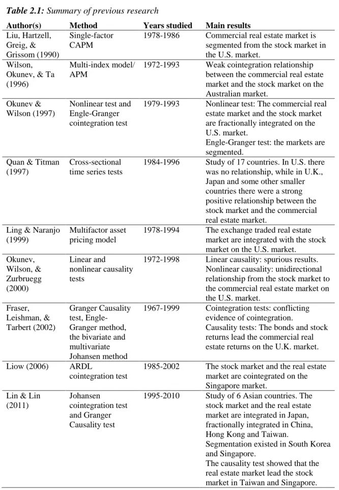
The previous studies of the relationship between the stock market and the real estate market have shown various and inconsistent results. The reasons for this may be because different time periods have been studied, the quality of data, the method(s) employed, and different economies and countries that may have differing political environment.

Table 2.1: Summary of previous research

Author(s) Method Years studied Main results

Liu, Hartzell, Greig, & Grissom (1990)

Single-factor CAPM

1978-1986 Commercial real estate market is

segmented from the stock market in the U.S. market.

Wilson, Okunev, & Ta (1996)

Multi-index model/ APM

1972-1993 Weak cointegration relationship

between the commercial real estate market and the stock market on the Australian market.

Okunev & Wilson (1997)

Nonlinear test and Engle-Granger cointegration test

1979-1993 Nonlinear test: The commercial real

estate market and the stock market are fractionally integrated on the U.S. market.

Engle-Granger test: the markets are segmented.

Quan & Titman (1997)

Cross-sectional time series tests

1984-1996 Study of 17 countries. In U.S. there

was no relationship, while in U.K., Japan and some other smaller countries there were a strong positive relationship between the stock market and the commercial real estate market.

Ling & Naranjo (1999)

Multifactor asset pricing model

1978-1994 The exchange traded real estate

market are integrated with the stock market on the U.S. market.

Okunev, Wilson, & Zurbruegg (2000) Linear and nonlinear causality tests

1972-1998 Linear causality: spurious results.

Nonlinear causality: unidirectional relationship from the stock market to the commercial real estate market on the U.S. market.

Fraser, Leishman, & Tarbert (2002) Granger Causality test, Engle-Granger method, the bivariate and multivariate Johansen method

1967-1999 Cointegration tests: conflicting

evidence of cointegration.

Causality tests: The bonds and stock returns lead the commercial real estate returns on the U.K. market.

Liow (2006) ARDL

cointegration test

1985-2002 The stock market and the real estate

market are cointegrated on the Singapore market.

Lin & Lin (2011)

Johansen

cointegration test and Granger Causality test

1995-2010 Study of 6 Asian countries. The

stock market and the real estate market are integrated in Japan, fractionally integrated in China, Hong Kong and Taiwan.

Segmentation existed in South Korea and Singapore.

The causality test showed that the real estate market lead the stock market in Taiwan and Singapore.

2.3 Relationship between Real Estates and Stock Returns

As this thesis examines the relationship between the stock market and the commercial real estate market it is essential to understand how the markets affect each other and also what external factors that can affect the markets in different directions.

Both the real estate market and the stock market are affected by economic activity, as well as they are affected by each other. Changes in real estate prices can lead to changes in the real economy through the interaction between the real estate market and equity markets along with housing markets and the motives of households’ precautionary savings. Gatson (2009) came up with three channels, the collateral, the lending and the household channel, that group the different effect of these interactions;

The collateral channel builds upon that a large downturn in the price of a collateralizable asset, such as real estate, is based on a decline in asset markets. This leads to negative effects of the company’s credit ratings and decreases its debt capacity, which in turn means that the company will not be able to make profitable investments and thus reduce its profits.

The lending channel describes how negative impacts of banks’ financial situations affect the real economy. This may be caused by a decrease in the assets markets. Since a large exposure of the banks’ balance sheets typically is to real estate markets, a significant change in real estate prices may be transmitted through banks’ decreased ability to lend to companies, which in turn forces the companies to forego profitable investments and therefore decreases the stock prices.

The household channel is comparable to the collateral channel because house owners are able to use their houses as security for financing of their households. An increase of real estate value typically leads to an increased consumption response since a household with limited liquidity can use the security of an increased value in their homes to finance consumption. However, Gan (2010) claims that the positive consumption responses only comes into effect after a sale or a refinancing of the house. Since this is something that does not occur frequently, a more likely reason to the increased consumption is that the precautionary savings motive decreases as the house prices increases.

Although some economic shocks are expected to cause the real estate market and the stock market to move in the same direction, there are other changes in the economy that are likely to cause the two markets to move in opposite directions. Quan & Titman (1999) state two possible reasons for the stock market and the real estate market to move in opposite directions. If companies have increased investment opportunities it may cause the stock prices to increase and thus lead to increased real interest rates, which in turn may cause the commercial real estate values to decrease, even if the rents in commercial real estates increases. Another economic activity that is likely to cause the two markets to move in opposite directions is if it exists some foreign competition, wages may be pressed down leading to increased profits for the companies but decreased values for the commercial real estates since the decrease in replacement values. Quan & Titman (1999) argue that these factors are of higher importance for the large and developed countries in North America and Europe, and in Japan than in smaller and undeveloped countries.

2.4 Modern Portfolio Theory

There are different theories of how to create a portfolio. We have chosen to use the Modern Portfolio theory presented by Harry Markowitz in 1952. This theory implies that a diversified portfolio will have the highest expected return with the lowest possible variance. The rule of this theory is to see the expected return as something wanted and the variance as something unwanted (Markowitz, 1952).

To create a portfolio the investor first needs to determine how much risk she is willing to take for her portfolio. Thereafter the investor is able to select different assets that suit her risk preferences. By investing some of the capital in each asset the investor will diversify her portfolio, and thus minimizing the risk. The selection of the assets needs to be done with careful consideration. By taking the co-movement between the assets into account the portfolio could be less risky. If the characteristics of the assets are identical with the characteristics of the portfolio the risk will not be reduced, since the portfolio return is the weighted average of the assets return. The risk of the portfolio on the other hand is not the weighted average of the assets and needs to be measured (Elton, Gruber, Brown, & Goetzmann, 2011).

The portfolio theory advises the investor to construct an efficient frontier, which shows the relationship between the risk and the return, with different portfolio opportunities. The minimum risk and the maximum expected return are at each of the ends on the efficient frontier (Markowitz, 1952) shown in Figure 2.1.

Figure 2.1: Efficient frontier for portfolios with multiple assets (authors own figure)

In Figure 2.1 there are different portfolio options. Portfolio B to D are efficient portfolios to invest in. The portfolio choice depends on the risk preference the investor has. A risk averse investor would prefer to invest in portfolio B since it has the lowest risk while an investor with a risk seeking preference would prefer portfolio D. Portfolio A is not efficient to invest in since portfolio C offers the same risk level but with a higher return (Elton, Gruber, Brown, & Goetzmann, 2011).

2.4.1 Portfolio Risk

When creating a portfolio it is important to consider different combinations of assets to be able to minimize the risk of the portfolio. By investing different proportions of the capital in each asset, the investor is able to diversify the portfolio and thus reduce some of the portfolio risk. To be able to create a well-diversified portfolio the investor should invest in assets within different industries since it is more likely that assets within the same industry generate poor returns at the same time. Another important term when discussing diversification of portfolio risk is covariance. Investing in assets that have

0 0,00005 0,0001 0,00015 0,0002 0,00025 0,0003 0,00035 0 0,005 0,01 0,015 0,02 0,025 0,03 Re tu rn Risk

Efficient Frontier

low covariance will also reduce the risk. Firms within the same industry tend to have a higher covariance than those assets that are operating in different industries (Markowitz, 1952).

Even though diversification can minimize the portfolio risk, all the risk cannot be diversified. The individual risk of each asset can be reduced by creating a well-diversified portfolio, while the market risk cannot be eliminated (Elton, Gruber, Brown, & Goetzmann, 2011). The individual risk, also called the non-systematic risk, is affected by firm-specific news, such as fluctuations in the stock’s return. This risk only affects the asset from the specific firm and it can be eliminated if the investor creates a well-diversified portfolio. The market risk, the systematic risk, on the other hand cannot be eliminated by diversification. Factors such as market-wide news on the whole economy, inflations, interest rates or natural disasters affect all firms and therefore also the whole stock market. It is therefore not possible to minimize this type of risk (Berk & DeMarzo, 2011).

2.4.2 Minimum Variance Portfolio

In this thesis we create a minimum variance portfolio, which is a combination of two or more assets. By including more than one asset to the portfolio the investor is able to reduce some of the risk. The minimum variance portfolio is used to generate a high expected return at the lowest possible risk. This type of portfolio is preferable for risk averse investors as they prefer as little risk as possible. The minimum variance portfolio is given by the equation:

𝑋_𝐶 = 𝜎𝑆 2_{− 𝜎} 𝐶𝜎𝑆𝜌𝐶𝑆 𝜎_𝐶2_{+ 𝜎} 𝑆2− 2𝜎𝐶𝜎𝑆𝜌𝐶𝑆 (2.1) Where 𝑋𝐶 is the weight of asset c in the portfolio, 𝜎𝑆2 and 𝜎𝐶2 are the variance of asset s

and c, 𝜎𝐶𝜎𝑆 are the standard deviation for each asset and 𝜌𝐶𝑆 is the correlation between

the assets. In this thesis asset c stands for commercial real estates and asset s for stock market (Elton, Gruber, Brown, & Goetzmann, 2011).

2.4.3 Risk Preferences

Any choice that does not have a certain outcome involves risk. Risk preference is someone’s tendency to select a certain amount of risk for a choice with an uncertain outcome. There are different types of risk preferences which are associated with how much risk the decision maker is willing to take on an investment.

A person with a risk averse preference does not like to invest in risky investments and does always choose the safe investment before taking chances to achieve high returns that involves the risk of failure.

The opposite of a risk averse preference is a risk seeking preference. A person that is risk seeking is willing to take more risk in order to achieve returns that are above the average. In order to decide if the risk is worth the chance, a person with risk seeking preferences weigh all the risk factors involved in the investment and evaluate these against the probabilities of different outcomes.

The last personality is a person that has a risk neutral preference. A risk neutral person is not concerned about how much or little risk that is involved in an investment, but only cares about the results in the end. A person with this kind of personality will select the investment that has the highest possible outcome without taking the risk of failure into account (Elton, Gruber, Brown, & Goetzmann, 2011).

2.4.4 Sharpe Ratio

To evaluate the portfolio we use the Sharpe ratio. This ratio measures the return compared to how much risk the investor has taken. The equation for the Sharpe ratio is:

𝑆ℎ𝑎𝑟𝑝𝑒 𝑟𝑎𝑡𝑖𝑜 =(𝑅̅𝑃−𝑅𝐹)

𝜎𝑃 (2.1)

Where 𝑅̅_𝑃 is the return for the portfolio, 𝑅_𝐹 is the risk free rate and 𝜎_𝑃 is the standard deviation for the portfolio.

If the Sharpe ratio is high it means that the return is high relative to the risk of the portfolio. Thus, a portfolio with a lower return can still spot a higher Sharpe ratio if the standard deviation is rather low. If the Sharpe ratio is negative this means that the return

of the portfolio has been lower than the risk free rate (Elton, Gruber, Brown, & Goetzmann, 2011).

2.5 Investment Alternatives

This thesis focuses on the direct investment of commercial real estates and stocks. However, there are different investment alternatives for the investors to choose among. It is important for investors to be aware of the characteristics of a direct commercial real estate investment as they differ from investments in both stocks and real estate funds.

2.5.1 Characteristics of a Direct Real Estate Investment

Direct investments in real estates are different from investments in other asset classes, such as investments in stocks and bonds. This is because real estates have some specific characteristics that distinguish them from other asset classes. Hoesli & MacGregor (2000) states some of the important features of a real estate investment;

First, real estates are unique and have its fixed location. Shares and bonds are identical, but there are no properties that are exactly the same as another property. They differ in size in land area and building, location, age, construction and maintenance. These factors are of high importance for the values of the property.

Second, the unit value of a property is very high. Unlike shares and bonds, which you can buy for a small amount of money, the direct purchase of real estates is very expensive and it is difficult for private investors and even for small institutions to construct diversified real estate portfolios. As a consequence of the high costs of investing in real estates, borrowing is an important part. However, to finance part of the investment with debt can be advantages for institutional investors because of the tax advantages.

Third, real estates require management during the whole period of the investment. Owning shares requires no liability of the investor, whereas real estates require the investor to manage everything from technical management, renovation, rent collection,

the leasing activities, to the transaction costs and the strategy to keep holding a well-diversified portfolio.

Fourth, there exists an information asymmetry in the real estate market. Prices on the stock market are decided by the interaction of many sellers and buyers in a central market. For the real estate market, there is no single trading market or central price listing and the price information available is therefore limited. An investor cannot get the price information from one transaction to use as a proxy for another property as all properties are unique and thus do not have the same value. Furthermore, the buyer typically has some information disadvantage since the seller of a property has more information than the potential buyer. Therefore, the buyer has to obtain knowledge from a professional valuer, which results in higher costs.

Lastly, the real estate market is illiquid and transaction costs are high. Often it can take several months to transact an asset. This is mainly because each property has a high unit cost, all properties are unique, it does not exist a single trading market to match sellers and buyers, and the negotiation between the seller and the potential buyers is time consuming.

2.5.2 Investment Alternatives in Real Estates

In Sweden, there are three investment alternatives in the real estate sector for the investor to choose between. One alternative is the direct purchase of a property which means that the investor has the rights of ownership to a land area, usually with a building (Hoesli & MacGregor, 2000). Another alternative is to invest indirect through a real estate fund, which in turn invests in real estates. This means that an investor can have a fraction of the real estate market in the portfolio without having to invest a large amount of money. The returns from both direct and indirect investments of real estates are generated through the appreciation of the property and a part of the return comes from the current earnings, for example the rental price. A third alternative is to invest indirect in real estates by investing in shares of listed real estate companies. However, this has been proven to give worse diversification effect to the portfolio as it has a higher correlation with the stock market (Public Banking, 2012).

Different investment alternatives are, however, more developed in other countries. In 1960, the congress in the U.S. created a real estate investment alternative called real estate investment trusts, REIT. It is a form of investment where there are a limited number of shares that the investors can purchase on central trading markets, such as the New York Stock Exchange. The purpose with REITs was to make real estate investments return available for investors without the resources to purchase property directly. One advantage with REITs is that it provides the investor with tax-related benefits as the investors does not have to pay any federal tax on income or capital gains, which cannot be offered through direct ownership of a property. Other advantages with REITs compared to direct investments in properties are that it is liquid and does not require any management. However, since REITs are traded at central trading markets, factors that are not related to the real estate market may affect the REIT stock prices, which in turn make the REITs more correlated with the stock market (Baker & Filbeck, 2013). Other countries that have REITs are Canada, Finland and Italy among others (Pwc, 2013). A similar form of investment was presented by Vinell (1996) where he suggested a Swedish solution to a new form of investment in real estates. His proposal was submitted as a motion to the parliament in 1996, but it has not yet been approved. However, this might be an alternative for investments in real estates in the future.

2.5.3 Investment Alternatives on the Stock Market

An investor that wants to invest in the stock market has several options. A common alternative is to purchase shares in a company. A share generates return based on the company’s profit after the creditors of the company have received their part (Sveriges Riksbank, 2013). Another investment alternative is funds. A fund is a portfolio of securities, such as stocks, and it is managed by a fund company that handles the investments and the administration. There are different types of funds, for example stock funds, interest funds, hedge funds and index funds (SEB).

One alternative that has become popular in recent years are exchange-traded funds (ETFs), which are baskets of underlying securities, commodities or fixed-income investments. Usually these funds are index funds. As stocks and funds, these are traded on the Stockholm Stock Exchange. An investment type that is not traded on any market

place is Contract For Difference (CFD). These are forward contracts without a maturity date and they reflect the changes in asset prices, usually consisting of shares, commodities or currencies (Sveriges Riksbank, 2013).

Many of the funds and the CFD contracts have an extra commission or brokerage fee, which might make the investment in shares a more attractive alternative (Sveriges Riksbank, 2013).

3 Method

In this chapter we present the research methodology and the data chosen. Further, we present the different methods and steps, which we use to answer our research questions.

3.1 Research Methodology

There are different types of research designs, such as descriptive, explanatory and exploratory (Blumberg, Cooper, & Schindler, 2008). The most appropriate research designs for the purpose of this thesis are to use a descriptive and an explanatory study. This will be done by performing statistical test in order to define whether there exist any relationship between the markets or not.

The perspective of the research can be either deductive, inductive or a combination of both (Blumberg, Cooper, & Schindler, 2008). This study is deductive as it is based upon previous research and leads the authors towards the result and the conclusion.

Quantitative and qualitative studies are two different research approaches to use when collecting and analyzing data. The main difference between these two studies is the kind of information that is used. A quantitative study is based on quantitative information, such as numbers that are statistically tested, while a qualitative study is based on qualitative information, for example, interviews (Blumberg, Cooper, & Schindler, 2008). The best suitable approach for this thesis is a quantitative study since the authors intend to use already existing data to perform correlation and cointegration tests.

3.2 Data

The data that will be used is secondary data collected from Thomson Reuters Datastream and Statistics Sweden. We used OMX Stockholm as a market proxy for the stock market and we chose two indices, sold multi-dwelling and commercial buildings and sold manufacturers industries, for the commercial real estate market. Since the commercial real estate market includes renting office buildings, retail premises, warehouse storages, and industry buildings it is preferable to study both the indices. It

could also be useful to study both indices to see if they distinguish from each other. When deciding which commercial real estate index to use in this thesis we chose between the indices of a direct investment and another index that consists of the largest listed commercial real estate companies. As the latter does not reflect the true commercial real estate values and is more correlated with the stock market we chose to use the indices that reflects the direct investments of commercial real estates.

The data that will be studied are quarterly and will be studied between the years 1994Q1 until 2013Q4. We believe that this time horizon investigated is sufficient as it covers the 1990s when the Swedish economy started to recover from the recession and the most recent crisis during 2007 and 2008.

3.2.1 OMX Stockholm

OMX Stockholm is a market index with all the listed companies on the Stockholm Stock Exchange and currently has 282 traded stocks (Nasdaq OMX Nordic, 2014). A common index to use as a market proxy is OMX Stockholm 30 but as it only covers the 30 most traded stocks it does not give a fair picture of the whole Swedish stock market. Therefore OMX Stockholm is an appropriate index to use in this thesis since this index includes all the stocks traded.

3.2.2 Sold Multi-dwelling and Commercial Buildings

Sold multi-dwelling and commercial buildings is one of the commercial real estate indices used in this thesis. The index is constructed by Statistics Sweden and it includes the average price for sold apartment buildings, offices and stores for each quarter. This index covers all purchases in the whole country and it is not weighted towards any specific geographical areas. Also, the prices are in nominal terms. This index does not include current earnings, such as rental prices, rather it reflects the real value of the appreciation of these commercial real estates. The index corresponds to a direct investment in commercial real estates and it is not exchange traded. Further in the thesis, this index will be referred to as commercial buildings.

3.2.3 Sold Manufacturers Industries

Sold manufacturers industries is the other commercial real estate index that we have used. This index is constructed in the same way as the sold multi-dwelling and commercial buildings index but instead it includes industry buildings. We will refer to this index as industry buildings.

3.2.4 Discussion of Data

The commercial buildings and the industry buildings indices are not weighted towards any specific geographical areas, which mean that there are large gaps in the prices between the cities and the countryside. Furthermore, the indices do not include rental prices, which are one of the main reasons to invest in commercial real estates. Therefore the results might be misleading and not give a fair view of the reality. However, commercial real estate indices in Sweden are limited. After careful consideration when choosing the indices we came to the conclusion that these two indices are the most appropriate for the purpose of this thesis, as the main purpose is to examine if there exists any relationship between the stock market and the commercial real estate market. Since there are some flaws with these indices, we choose to compare the results with another commercial real estate index conducted by IPD (IPD, 2013). This index includes the total percentage return, both appreciation and the direct return, such as rent. However, the index only contains yearly returns and is therefore not suitable for performing cointegration, correlation and lead-lag relationship tests as these tests requires a certain number of observations. Even though, it can be useful to compare and discuss this index with the results from our own tests.

3.3 Cointegration

Testing for cointegration can be used to forecast future time series. In this thesis we will use cointegration tests to investigate if there exist any long-term relationship between OMX Stockholm and the commercial real estate indices. This relationship exists when the two time series move closely together and they appear to have the same stochastic

trends. If a linear combination of the times series is stationary the markets are cointegrated. Time series that are non-stationary can move together in the long-run because they are affected by macroeconomic factors, and thus, are bounded by a relationship. It is also possible that the markets show no relationship in the short-run, but it appears in the long-run, thus indicating that the markets are cointegrated (Brooks, 2008).

3.3.1 Stationarity

To get a trustworthy result from the cointegration tests, it is important to state whether the data is stationary or non-stationary, since we then should treat the data differently. In the case where the data are stationary, this means that the mean, the variance and the autocovariances are constant for each given lag. Hence, it means that the future does not differ from the past, in a sense of probability distribution. On the other hand, if the data are non-stationary this implies that the data in period one are not related to the next period of the data. This in turn can lead to a spurious regression (Brooks, 2008). If the two markets are non-stationary and follows a stochastic trend over time they can show a close relation even though the markets are not related (Stock & Watson, 2012).

If the data is non-stationary it has to be transformed to become stationary. This is done with the following equations:

𝑦𝑡 = 𝑦𝑡−1+ 𝑢𝑡 (3.1)

Where 𝑦𝑡 is the data of one market at time t, 𝑦𝑡−1 is the data of one market one period

previous of time t, and 𝑢_𝑡 is a white noise error term. By subtracting 𝑦_𝑡−1 from both sides in equation 3.1 we will get:

∆𝑦𝑡= 𝑢𝑡 (3.2)

The new variable ∆𝑦𝑡 is now stationary and has no unit root. Depending on how many

unit roots the non-stationary data has, this will determine how many times it needs to be differenced. By applying these equations d number of times, it leads to an I(0) process, which is a stationary series with no unit roots. A series with I(1) means that it is

integrated of order one, thus contains one unit root and to become stationary it needs to be differenced once (Brooks, 2008).

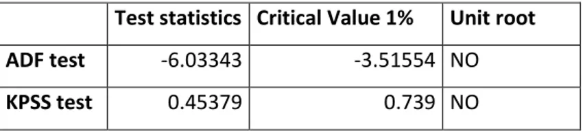
To test for the degree of unit roots in OMX Stockholm and the commercial real estate indices the augmented Dickey-Fuller (ADF) test and the Kwiatkowski-Phillips-Schmidt-Shin (KPSS) test will be used. By performing both tests it will provide us with a more reliable result.

The null hypothesis of the ADF test is ψ = 0, which means that the data contains a unit root, against the alternative hypothesis that the data has no unit root and is therefore stationary. To reject the null hypothesis the t-statistic has to be more negative than the critical values for Dickey Fuller tests at a significance level of 1 %. The test is performed with the following equation (Brooks, 2008):

∆𝑦_𝑡= ѱ𝑦_𝑡−1+ ∑ 𝛼_𝑖∆𝑦_𝑡−1+ 𝑢_𝑡

𝑝

𝑖=1

(3.3) Where α is an unknown coefficient and p is the number of lags in the regression. The number of lags can be determined by either Akaike information criterion (AIC) or the Bayes information criterion (BIC). The difference between these two models is that with AIC the number of lags will be more than with the BIC. We will use the AIC model as it is recommended to have more lags when performing an ADF test. It is essential to use the right amount of lags since too few does not reduce the autocorrelation whereas too many will increase the uncertainty.

The formula for AIC is (Stock & Watson, 2012):

𝐴𝐼𝐶(𝑝) = ln [𝑆𝑆𝑅(𝑝)_𝑇 ] + (𝑝 + 1)2_𝑇 (3.4) Where 𝑆𝑆𝑅(𝑝) is the sum of the squared residuals of an autoregression and T is the number of observations.

The KPSS test is also a test for stationarity. The difference between this test and the ADF test is that the null and the alternative hypothesis are reversed (Brooks, 2008). It has been found evidence that standard test of stationarity, like the ADF test, tend to fail

to reject the null hypothesis, that the data contains a unit root, because there has to be strong evidence against the null hypothesis. The KPSS test is therefore a good complement to the ADF test since we then test both the null hypothesis that the data is stationary and the null hypothesis that the data contains a unit root (Kwiatkowski, Phillips, Schmidt, & Shin, 1992). To get a robust result of the two tests the outcome should be that one of the tests rejects the null hypothesis and the other test accepts the null hypothesis (Brooks, 2008).

3.3.2 The Engle-Granger 2-step Method

The Engle-Granger method is one method to use to examine if the stock market and the commercial real estate market are cointegrated. This method is used to measure if there is any stochastic trend in the time series (Brooks, 2008).

The first step in this method is to make sure that OMX Stockholm and the commercial real estate indices contain one unit root, which is done by performing the ADF and the KPSS tests. By running the OLS cointegration regression, the parameter values, β1 and

β2, and the residuals will be estimated. We will run the OLS regression twice for each

combination to have both indices as dependent and independent variables to get a more robust result. If the residuals in the OLS regression model are stationary one can proceed to the second step. To test the stationarity we will use the ADF and the KPSS tests. If the residuals contains one unit root there is no cointegration relationship between the variables.

In the second step the residuals from step one are put in the error correction model: ∆𝑦_𝑡 = 𝛽₁∆𝑥_𝑡+ 𝛽₂(û𝑡−1) + 𝑣𝑡 (3.5)

Where û_𝑡−1 is equal to 𝑦_𝑡−1− 𝜏𝑥_𝑡−1 and 𝑣_𝑡 is the error correction. The 𝜏 is known as the cointegrating vector, which measures the long-run relationship between the markets (Brooks, 2008).

3.4 Correlation and Standard Deviation

In this thesis we investigate if there is any correlation between the commercial real estate market and the stock market in order to see if there exists any short-run relationship between the two variables.

Correlation measures if there is a linear relationship between two variables, where the correlation coefficient is somewhere on a scale from -1 to +1. It describes the average relationship from one observation to the next observation, which in this study is quarterly. A correlation coefficient equal to zero would mean that there is no relationship between the variables. If the correlation coefficient is equal to one the linear relationship between the variables are perfect. This means that if one of the variables increases the other variable also increases. When the correlation coefficient is equal to minus one there is a perfect negative relationship, which means that the variables are moving in perfect opposite directions (Aczel & Sounderpandian, 2009). If this is the case an investor have the opportunity to create a diversified portfolio with no risk. The correlation coefficient (p) is calculated by using the following formula (Aczel & Sounderpandian, 2009):

𝑝 =𝐶𝑜𝑣(𝑅𝑥,𝑅𝑦)

𝜎𝑥𝜎𝑦 (3.6)

Where 𝐶𝑜𝑣 is the covariance, 𝑅𝑥 and 𝑅𝑦 are the average returns on the commercial real

estate market and the stock market, and 𝜎𝑥 and 𝜎𝑦 is the standard deviations of the two

markets. The standard deviation measures the spread of the data around its mean. A high standard deviation is an indication of high uncertainty of the investment.

The correlation coefficient along with standard deviation can be used to calculate the standard deviation of a multi-asset portfolio. By creating a portfolio with shares of the commercial real estate indices and shares of the OMX Stockholm an investor can choose a portfolio with low standard deviation and thus minimizing the risk in relation to the return. If the two assets have a low correlation the standard deviation in the portfolio will be lower because the investments do not move together (Elton, Gruber, Brown, & Goetzmann, 2011).

3.5 Test for Lead-lag Relationship

The Granger causality test is used to test the hypothesis that changes in the commercial real estate return is lagged by changes in the stock market returns. The F-statistic of a time series regression with multiple predictors tests the null hypothesis that the lags of one variable have no predictive content over the other variable in the model. The equation for the time series regression with multiple predictors is (Stock & Watson, 2012):

𝑦𝑡= 𝛽0+ 𝛽1𝑦𝑡−1+ 𝛽2𝑦𝑡−2+ ⋯ + 𝛽𝑝𝑦𝑡−𝑝+ 𝛿1𝑥𝑡−1+ 𝛿2𝑥𝑡−2+ ⋯ + 𝛿𝑞𝑥𝑡−𝑞+ 𝑢𝑡

(3.7) Where 𝑦_𝑡 is the stock market at time t, 𝑥 is the commercial real estate market, 𝛽 and 𝛿 are unknown coefficients for the variables, 𝑝 and 𝑞 are the number of lags, and 𝑢𝑡 is the

error term.

The Granger causality does not in fact really indicate causality, but the test is more used to see if a lead-lag relationship exists (Stock & Watson, 2012). If there exist Granger causality between commercial real estates and the stock market the strength of accepting a low or negative correlation weakens, hence the diversification benefits weakens. Investors with a short investment horizon could still take advantage of an existing lead-lag relationship. For example, if commercial real estate returns lead-lag the stock market by a year an investor with a shorter time horizon could benefit from holding a multi-asset portfolio.

3.6 Discussion of Methods

When testing for unit roots we have chosen to use the ADF test and the KPSS test. Though, there also exists a unit root test called Phillips-Perron (PP). The ADF test and the PP test are very similar to each other as they often generate the same conclusions and they suffer from the same limitations. Therefore it is not necessary to conduct both these tests. The criticism of the ADF and the PP tests is that it is difficult to reject the null hypothesis, due to insufficient information in the sample. To avoid this problem we will perform both the ADF test and the KPSS test as the hypotheses of these tests are