Master’s Thesis in Environmental Science
Carbonaceous aerosols and trace metal deposition in
high-latitude snow –
A comparative study in Sweden and Alaska
Anika Pinzner
Carbonaceous aerosols and trace metal deposition in
high-latitude snow –
A comparative study in Sweden and Alaska
Anika Pinzer
Supervisor: Youen Grusson, Department of Soil and Environment, SLU Assistant supervisor: Anders Svensson, University of Copenhagen, Niels Bohr Institute, Center for Ice and Climate
Assistant supervisor: Christian Zdanowicz, Department of Earth Sciences, Uppsala University
Assistant supervisor:Martin Stuefer, Geophysical Institute, Atmospheric Sciences University of Alaska Fairbanks,
Examiner: Jon Petter Gustafsson, Department of Soil and Environment, SLU Credits: 30 ECTS
Level: Second cycle, A2E
Course title: Independent Project in Environmental Science – Master´s thesis Course code: EX0431
Programme/Education: EnvEuro – European Master in Environmental Science 120 credits Course coordinating department: Soil and Environment
Place of publication: Uppsala Year of publication: 2019
Cover picture: 2017, Denali National park, photo by: Anika Pinzer Title of series: Examensarbeten, Institutionen för mark och miljö, SLU Number of part of series: 2019:07
Online publication: http://stud.epsilon.slu.se
Keywords: now, PM, carbon particles, pXRF, Arctic, subarctic, EC/OC, LAHM, PSAP, TOT, ICP-MS, filter, contamination, albedo
Abstract
This study investigates the advantages and disadvantages of several destructive and non-destructive analytical methods that can be employed to characterize airborne par-ticulate matter (PM) deposited in seasonal snow. To this end, a comparative study was conducted on PM obtained from snowpack surveys in two Arctic/subarctic re-gions of Northern Sweden and Interior Alaska, USA. This study measured and char-acterized carbonaceous particles (CPs) in snow-filtered PM using three different op-tical analyop-tical methods: a Particle Soot Absorption Photometer (PSAP), a Thermo-Optical Transmittance (TOT) analyser, and a Light-Absorbing Heating Method (LAHM) instrument. The study additionally tested the applicability of a portable X-Ray Fluorescence (pXRF) analyser for quantifying the particulate trace metal content in the snow. The ratios of analytes from the measurements performed with the pXRF were also compared with the ratios of elements from bulk chemical analyses by In-ductively Coupled Plasma Mass Spectrometry (ICP-MS). Snow meltwater was fil-tered with two filtration set-ups (syringe and vacuum-pump) on two differently sized tissuquartz filters (25 mm and 50 mm). The analysis of CPs suggests a higher corre-lation between the measurements of PSAP/TOT in comparison to LAHM/TOT meas-urements. The lower association between LAHM and TOT were i.a. assumed to de-rive from heterogeneities of the loading of the filter material especially on the smaller 25 mm filters produced by syringe-filtration. Organic carbon (OC) and elemental carbon (EC) values derived from TOT measurements gave insight into possible emis-sion sources in different geographic regions of Sweden and Alaska. High OC values in rural Alaska suggested the influence of wood smoke on the particle composition in the snow. The chemical analysis of the empty and blank tissuquartz filters used for filtration showed high base elemental concentrations. Despite these high initial val-ues of the filter matrix, an analysis of the two inbuilt calibrations ‘GeoMining’ and ‘GeoExploration’ showed that both calibrations measure relatively precisely. pXRF calibration ‘GeoExploration’ further yielded higher count rates and thus is more suit-able for trace metal analysis filters than calibration ‘GeoMining.’ The correlation of ICP-MS vs. pXRF further showed no significant relationship between the measure-ments of the two methods. Yet, for filters with high filter loadings the relative con-centration pattern (RCP) of the pXRF measurements reflected the chemical compo-sition of the respective sample environment. This suggests that further investigations into using pXRF for snowpack analyses could be a valuable time- and cost-effective tool for the analysis of chemical composition of snow.
Keywords: PM, carbon particles, trace metals, pXRF, Arctic, subarc-tic, EC/OC,
Snow has many important functions: It serves as animal habitat, enables transporta-tion (e.g. by dogsled), regulates the climate and yields water for almost two billion people worldwide. Even though snow is primarily composed of water, snow-flakes can scavenge small particles emitted by natural or anthropogenic sources and deposit them on the snowpack. Such particles, also called particular matter (PM), can also be deposited via settling of particles on the snow or other forms of dry deposition. Of concern are particles which contain carbon, and which are therefore dark in colour. Dark particles take up more energy than ice crystals in snow and can therefore lead to an earlier beginning of the snow melt season. Another concern is the level of trace metals in PM which, in certain amounts, can be toxic to humans, animals, and plants once released to streams and waterbodies.
To analyse and characterize the different components of PM in snow, snow sam-ples were taken in Northern Sweden and Interior Alaska in places with varying hu-man influence and proximity to different emission sources. The snow was subse-quently melted and filtered with two different filtration set-ups and the resulting loaded quartz filters were analysed using five methods. To measure carbonaceous particles (CP) in snow, three methods were applied, and the respective results com-pared. The methods were based on different physical principles (thermal or optical), and thus introduced different uncertainties into their measurements. It was found that a lesser load of particles on the filters is preferable for the analysis of CP. Snow sam-ples were screened for trace metals using two methods, one of which was rather ex-ploratory in design, as the respective method hasn’t been widely applied to such filter material yet. Some of the snow samples showed concerning high concentrations of certain elements which could be related to the environmental setting in which the samples were taken. It was also shown that filtering snow meltwater with a vacuum pump instead of a syringe produced more homogeneous filter loadings.
Due to the increase of human activities in Arctic and subarctic regions and the important ecosystem functions of snow, quantifying the different impurities in snow can help increase understanding and prediction of snow melt rates as well as ecosys-tem responses to change.
I, Anika PINZNER, declare that this thesis titled, “Carbonaceous aerosols and trace metal deposition in high-latitude snow: A comparative study in Sweden and Alaska” and the work presented in it are my own.
I confirm that:
• This work was done wholly or mainly while in candidature for a research degree at the above-mentioned Universities.
• Where I have consulted the published work of others, this is always clearly attributed.
• Where any part of this thesis has previously been submitted for a degree at this University or any other institution, this has been clearly stated. • Where I have quoted from the work of others, the source is always given.
With the exception of such quotations, this thesis is entirely my own work. • I have acknowledged all main sources of help.
Signed:
Date:
List of tables 10
List of figures 12
Abbreviations 15
1 Introduction 19
1.1 Motivation and Objectives 21
2 Background 23
2.1 Atmospheric Pathways to the Northern Regions 24 2.2 Deposition of Atmospheric Particulate Matter on Snow 28 2.3 Atmospheric particulate metals in northern regions 28 2.4 Carbonaceous aerosols in northern regions 31
3 Terminology 36
3.1 Environmental Contamination and Pollution 36
3.2 Trace or ‘Heavy’ Metals 36
4 Study Area 38
4.1 Northern Sweden 38
4.1.1 Climate 38
4.1.2 Snow Conditions 39
4.1.3 Surficial Materials and Soil Chemistry 40 4.1.4 Pollution Sources: Local and Global 40
4.2 Interior Alaska 42
4.2.1 Climate 42
4.2.2 Surficial Materials and Soil Geochemistry 44
4.2.3 Snow Conditions 44
4.2.4 Pollution Sources: Global and Local 45
5 Materials and Methods 48
5.1 Site Description 48
5.1.1 Northern Sweden 48
5.1.2 Interior Alaska 51
5.2 Snow Sampling 57
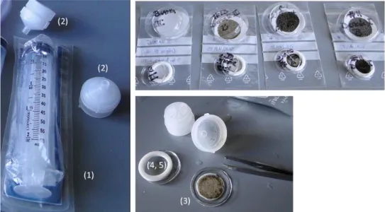
5.3 Filtration Procedure and Filter Handling 57
5.3.1 Vacuum pump filtration set-up (50 mm filters) 58 5.3.2 Syringe filtration set-up (25 mm filters) 59
5.4 Laboratory Analysis 60
5.4.1 Methods for the detection of carbonaceous particles 60 5.4.2 Methods to for the detection of trace elements 64
5.5 Statistical and Graphical Analysis 66
6 Results and Discussion 68
6.1 Analysis of Carbon Particles 68
6.1.1 Method comparison: TOT vs PSAP and TOT vs LAHM 69 6.1.2 Comparison of CP levels: Northern Sweden and Interior Alaska 72 6.1.3 CP in N. Sweden and I. Alaska within the Arctic/subarctic context 79
6.2 Analysis of trace elements 82
6.2.1 Element concentration on blank and empty filters 82 6.2.2 Coefficient of variation analysis of pXRF measurements 87
6.2.3 Effects of pXRF calibrations 91
6.2.4 Geographic categorization – pXRF measurements 93 6.2.5 Source and environmental categorization – pXRF 97 6.2.6 Comparison of pXRF and ICP-MS 104
7 Conclusion 109
References 111
Acknowledgements 123
Table 1. Sets of tissuquartz filters measured by the TOT, PSAP, and LAHM
method for filter sets AK25, AK50, SW50 69 Table 2. Correlation coefficient R and coefficient of determination R² for RMA
regression of PSAP/TOT and LAHM/TOT. 69 Table 3. OC and EC values for Swedish and Alaskan snow samples and their
respective environmental setting and CP source categories 74 Table 4. Descriptive statistics of OC and EC concentrations for geographic
categories of the two regions Alaska and Sweden 75 Table 5. OC/EC ratios for Interior Alaska and Northern Sweden 77 Table 6. EC concentrations of ‘remote’ Alaska and Sweden samples as well as
mean EC concentration of both regions 80 Table 7. CV values of pXRF measurements sorted according to analyte for
each of the filter sets and calibrations 90 Table 8. Correlation coefficient R and coefficient of determination R² for the
RMA regression of the methods pXRF and ICP-MS for both regions 106
Appendix - Tables
Table A.1. Coefficients of Variation for filter set AK25E 131 Table A.2. Coefficients of Variation for filter set AK25M 132 Table A.3. Coefficients of Variation for filter set AK50E 133 Table A.4. Coefficients of Variation for filter set AK50M 134 Table A.5. Coefficients of Variation for filter set SW50SE 135 Table A.6. Coefficients of Variation for filter set SW50SM 136
Table A.7. Coefficients of Variation for filter set SW50SME and SW50SMM 137 Table A.8. Coefficients of Variation for filter set SW50DE and SW50DM 138 Table A.9. Coefficients of Variation for filter set AK25BLE, AK25BLM,
AK50BLE, AK50BLM, EME, and EMM 139
Table A.10. LODs for Tracer 5i GeoExploration and GeoMining calibration 140
Figure 1. The Arctic/subarctic region 23 Figure 2. Positive and negative AO phases since 1965 25
Figure 3. The Atlantic Oscillation 26
Figure 4. The major physical pathways of contaminants to the Arctic 27 Figure 5. Total annual deposition of lead to the Arctic in 1990 30 Figure 6. Surface concentration of black carbon for average of AeroCom models 32 Figure 7. Snow sample locations of previous field campaigns 34 Figure 8. Map of Sweden with sample region marked with black box 38
Figure 9. Thematic maps of Northern Sweden 39
Figure 10. Climate maps of the snow cover in Northern Sweden 39 Figure 11. Snow depth in Northern Sweden in 2017 40
Figure 12. Mines in Northern Sweden in 2018 41
Figure 13. Map of Alaska with sample region 42
Figure 14. Mean Annual Temperature Alaska 42
Figure 15. Downscaled projections of rain/snow partitioning for Alaska shown as
Snow-day Fraction 43
Figure 16. Mean Annual Precipitation Alaska 43
Figure 17. Snow water equivalent Alaska 45
Figure 18. Last day of spring snow cover Interior Alaska 2016 with schematic delineation of the large-scale geographic regions 45 Figure 19. Mines and Mineral Deposits in Interior Alaska 46 Figure 20. Sample sites with sample-IDs in Northern Sweden 49
Figure 21. Snow sampling site in Umeå 50
Figure 22. Sample sites with sample-IDs in Interior Alaska 52
Figure 23. Cleary Summit in sight of the Fort Knox gold mine 53
Figure 24. Healy coal power plant 53
Figure 25. Sample location A21 along the US Creek Road 56 Figure 26. Vacuum pump filtration set-up with 50 mm tissuquartz filters and filters
after snow meltwater filtration. 58
Figure 27. Syringe filtration set-up with 25 mm tissuquartz filters and filters after
snow meltwater filtration. 59
Figure 28. Example thermogram from analysis of OC and EC 61 Figure 29. A schematic cross-section of the PSAP 62
Figure 30. LAHM instrument set-up 63
Figure 31. Measurement set-up of the pXRF instrument Tracer 5i from Bruker 64 Figure 32. Schematic display of the measurement point on the different filters 65 Figure 33. Reduced Major Axis regression of TOT/PSAP 72 Figure 34. Reduced Major Axis regression of TOT/LAHM 72 Figure 35. OC, EC, mean TC concentrations and OC/EC ratios of Interior Alaska
and Northern Sweden according to geographic settings 78 Figure 36. OC, EC, mean TC concentrations and OC/EC ratios of Interior Alaska
and Northern Sweden according to the dominant CP source of
emission 79
Figure 37. BC concentrations in the Arctic/subarctic region 81 Figure 38. Mean trace metal levels of filter batch No. 3167 of MK 360 filters as
provided by Munktell Ahlstrom product catalogue 84
Figure 39. Measurements of empty filter #9 84
Figure 40. Measurements from nine empty filters measuring with calibration
GeoExploration and GeoMining 86
Figure 41. pXRF results from blank II of both filter sizes 87 Figure 42. Box-and-Whisker plots for CVs of the different sets of filters 89 Figure 43. Box-and-Whisker plots for CVs sorted by analytes 92 Figure 44. Levels of trace elements of all filters of each calibration run sorted by
analytes 92
Figure 45. Relative abundance of the log-transformed trace element
concentrations for Sweden 95
Figure 46. Mean trace element levels of calibrations GeoExploration and
GeoMining for sample JK01 95
Figure 48. Mean trace element levels of calibrations GeoExploration and
GeoMining for sample A12 DPR III 97
Figure 49. Relative abundance of trace elements for Sweden 98
Figure 50. Close-up of figure 49 99
Figure 51. Relative abundance of trace elements for Alaska 100
Figure 52. Close-up of figure 51 101
Figure 53. Mean trace element levels of calibrations E and M for samples A13 AIR, A14 AIR_L, and A22 AIR_C for both filter sizes 103 Figure 54. Levels of trace elements measured with all calibration runs for both
calibrations for sample A4 50 mm 104
Figure 55. Mean trace element levels of calibrations GeoExploration and
GeoMining for sample A23 for both filter sizes 101 Figure 56. Reduced Major Axis (RMA) regression fitted to the pXRF and ICP-MS
analyte ratios from Sweden and Alaska for both calibrations 108
Appendix - Figures
Figure A.1. Global short-lived climate pollutant (SLCP) emissions 124 Figure A.2. Mean trace metal levels of filter batch No. 3167 125 Figure A.3. Typical Levels of Trace Elements on empty filters (catalogue) 126 Figure A.4. Trace element values of blank filters of both sizes 127 Figure A.5. Coefficient of Variation values of every filter in every set of filters
ordered by element 128
Figure A.6. Log-trans. trace elements levels for SW/ source categorization 128 Figure A.7. Log-trans. trace elements levels for AK/ source categorization 129 Figure A.8. Log-trans. trace elements levels for AK/ source categorization 134
AC Atmospheric Circulation
Al Aluminium
AK Alaska
AMAP Arctic Monitoring and Assessment Programme AO Arctic Oscillation
Ar Argon
ARM Atmospheric Radiation Measurement
As Arsenic
Ba Barium
BC Black Carbon
BCe Black Carbon equivalent
Ca Calcium
Cd Cadmium
CO Carbon monoxide
CP Carbon/ carbonaceous particle
Cu Copper
Cr Chromium
CV Coefficient of variation
DI Deionized
E GeoExploration
eBC Equivalent Black Carbon
EC Elemental Carbon
EDXRF Energy dispersive X-Ray Fluorescence EEA European Environmental Agency
EPA United States Environmental Protection Agency Est.BC Estimated Black Carbon
Fe Iron
H2O2 Hydrogen peroxide
HF Hydrofluoric acid
Hg Mercury
HNO3 Nitric acid
ICP-QP-MS Inductively Coupled Plasma Quadrupole Mass Spectrometer IUPAC International Union of Pure and Applied Chemistry
K Potassium
LAHM Light-Absorption Heating Method LAI Light absorbing impurity
LED Light emitting diode LOD Limit of Detection
LRTAP Long-Range Transboundary Air Pollution
M GeoMining
MAC Mass absorption cross sections
MD Mineral Dust mL Millilitre Mg Magnesium Mn Manganese MS Mass Spectrometry Na Sodium Ni Nickel
NSIDC National Snow & Ice Data Center NOX Nitrogen oxides NO3- Nitrate O3 Ozone OC Organic Carbon Pb Lead PM Particulate Matter Ppm Parts per million
PSAP Particle Soot Absorption Photometer pXRF portable X-Ray Fluorescence
Rb Rubidium
RCP Relative concentration pattern
Refl Reflectance
RSD Relative standard deviation SD Standard deviation
Sb Antimony
Se Selenium
SLCP Short-lived Climate Pollutant
SO2 Sulfur dioxide
SO42- Sulfate
Sr Strontium
SW Sweden
SWE Snow water equivalent
TC Total Carbon
TOT Thermal-Optical Transmittance Trans Transmittance
USGS U.S. Geological Survey
V Vanadium
VOCs Volatile Organic Contaminants WHO World Health Organization
The changing state of the global atmosphere has received a great deal of scien-tific and, increasingly, political attention during the last decades. Rising global tem-peratures caused by ‘climate forcers’ such as atmospheric levels of carbon dioxide (CO2), methane (CH4) and ozone (O3) have been the focus of climatic concerns. In
parallel with this, there has also been a growing concern about deteriorating air qual-ity in many parts of the world, which affects climate as well as the health of humans and that of the ecosystems they depend upon. According to new data from the World Health Organization (WHO), nine out of ten people worldwide breath contaminated air, with an estimated 4.2 million premature deaths per year caused by ambient air pollution alone (WHO, 2018). The United States Environmental Protection Agency (EPA) identifies six ‘criteria air pollutants’, which are deemed specifically harmful to human health and the environment (EPA, 2018). Besides noxious gases such as sulphur dioxide (SO2), carbon monoxide (CO) and nitrogen oxides (NOX),
ground-level O3, lead (Pb) and particulate matter (PM) are cited on the infamous list (ibid;
NIH, 2018).
In this context, PM or aerosol describe a mixture of both solid and liquid particles suspended in air, such as soot, dust, or smoke, which can be either natural or emitted from anthropogenic sources (UCAR, 2019; EPA, 2018). These particles or droplets can vary greatly in size, with some particulates being so big and dark that they create a haze which is visible to the naked eye, while others can only be detected through an electron microscope (EPA, 2018; IVHHN, 2018). Despite their differences in chemical composition and surface properties, a distinction is oftentimes made be-tween inhalable particles with a diameter <10 µm (PM10) and particles with a
diam-eter <2.5 µm (PM2.5). The sources of aerosol are manifold: some are emitted directly
in particulate form from sources such as forest fires, soil dust, sea spray, mines or smokestacks (primary aerosols), while others are formed as a result of chemical re-actions between gaseous pollutants in the atmosphere, emitted e.g. by cars, indus-tries or power plants (secondary aerosols) (UCAR, 2019). In addition to the
amplify heart diseases, some aerosols can consist of, or contain, toxic substances. Examples include certain toxic metals, which can be associated with power plant or vehicular emissions, and volatile organic contaminants (VOCs) such as carcino-genic benzopyrene, often associated with soot (Valavanidis et al., 2008; Dickhut et al., 2000).
The geographic dispersion of polluting aerosols is partly determined by their size and partly by prevailing weather conditions. Gravity forces larger particles to quickly settle to the ground near emission sources (gravitational settling), mostly in a matter of hours, whereas smaller and lighter particles (~<1 µm), can stay sus-pended in air for weeks and months at a time and thus travel much longer distances (102 -103 km; UCAR, 2019). Some aerosols, such as black carbon (BC; a refractory type of soot) can be efficiently removed from the atmosphere by wet deposition in rain, fog droplets, ice grains, or snow (Paramonov et al., 2011). Snowflakes are es-pecially efficient aerosol scavengers and even a moderate snowfall can deposit a substantial number of particulates on the ground surface (Bourgeois & Bey, 2011). At its annual peak extent, the perennial and seasonal snow cover occupies ~30% Earth’s surface (NSIDC, 2019). It is an important natural resource having great im-pact on Earth’s global and regional climate (Mankin et al. 2015), supporting a unique ecosystem (Callaghan et al., 2011; Starr and Oberhauser, 2003), and impact-ing economic livelihoods (Ghaderi et al., 2013). Seasonal snowpacks constitute a vital source of drinking water (NSIDC, 2019) with about 1.9 billion people world-wide depending heavily on runoff from snowmelt (Mankin et al., 2015). However, the expanding global human population, increasing fossil fuel soot emissions, in-creasing anthropogenic activities (e.g., resource extraction), and a warming climate are now raising concerns about rising urban and rural pollution levels in snow and snow meltwater (Law and Stohl, 2007). Airborne contaminants deposited over the course of a single year (seasonal snow) or several years (perennial snow) can be released by melt into surface waters or undergo chemical transformations creating different types of hazardous contaminants, such as the toxic metal mercury (Hg) which can be subject to transformations to form the potent neurotoxin methylmer-cury (MeHg) (Dupuis, 2017; Larose et al., 2013). Additionally, light-absorbing (i.e., dark) airborne PM, such as dust or soot, deposited on snow alters the radiative prop-erties of snowpacks which can lead to significant increases in melt rates, particularly in spring (Schmitt et al. 2015). The amount and the different types of PM deposited on snow cover may vary with geographical location, meteorological conditions and atmospheric composition (Paramonov et al., 2011). In certain regions such as the Arctic or the Andes, the accumulation of PM on snow can have significant impacts on both people and ecosystems considering the multitude of functions and ecosys-tem services of snow as well as its widespread distribution. With the rapidly chang-ing climate in the high-latitudes human activities in those regions are expected to
increase substantially in the near future, which gives rise to concerns of increasing snow cover pollution in the Arctic and subarctic regions (Huntington et al., 2007).
1.1 Motivation and Objectives
Sources of airborne contaminants and their transport pathways to the polar re-gions have been the subject of several studies (Fischer, 2011; CACAR II, 2003; AMAP, 1998; Barrie et al. 1992). Particulate contaminants deposited in the snow-pack can affect its physical properties (e.g., albedo) and be released in snowmelt, adversely impacting freshwater and marine ecosystems (AMAP, 1998). This is of particular concern for local populations, who may be exposed to hazardous levels of contaminants in drinking water or in their traditional fish/game diet. Light-ab-sorbing impurities (LAIs) deposited in snow may also hasten snow melt onset in northern regions, which can have both local (hydrological) and global (albedo feed-back) impacts.
The perennial and seasonal snow cover is widespread at high latitudes in winter, which makes it a convenient sampling medium to investigate geographical differ-ences in the deposition of airborne particulate contaminants (Orr et al., 2019). How-ever, at present few comprehensive surveys of airborne particulate matter (PM) in snow exist for the Arctic and subarctic regions. Existing published surveys of this sort are primarily local in character and have been carried out using a variety of methods, making any intercomparison difficult (Caritat et al., 2005). Systematic sur-veys of airborne PM in snow across parts of the Arctic and/or subarctic using stand-ardized protocols would give deeper insight into inter-annual and spatial trends in PM deposition, and can be used to validate air pollutant model simulations. Findings can also inform policy makers on the efficacy of atmospheric pollution reduction measures and help local northern communities to anticipate the impact of possible changes in snow cover duration and melt onset.
This study investigates the pros and cons of several destructive and non-destruc-tive analytical methods that can be employed to characterize airborne PM deposited in seasonal snow. To this end, a comparative study was conducted on PM obtained from snowpack surveys in two Arctic/subarctic regions of Northern Sweden and Interior Alaska, USA. These two regions are affected by different local and distant sources of natural and anthropogenic contaminants (e.g., residential heating emis-sions of soot). The first objective of the study was to measure and characterize car-bonaceous/ carbon particles (CPs) in snow-filtered PM using three different optical analytical methods: a Particle Soot Absorption Photometer, a Thermo-Optical Transmittance (TOT) analyser, and a Light-Absorbing Heating Method (LAHM). The second objective of this study is to the test the applicability of a portable X-Ray
Fluorescence (pXRF) analyser for quantifying the particulate trace metal content in the snow. The presence of particulates emitted either naturally or through human activity can affect estimates of the radiative impact of CPs in snow. Measurements performed with the pXRF were also compared with bulk chemical analyses by In-ductively Coupled Plasma Mass Spectrometry (ICP-MS), which is a standard method for quantifying the trace metal composition in PM.
The key research questions of this study are:
i) What is revealed about CP in snow when considering different techniques (TOT vs PSAP, TOT vs LAHM), especially regarding the incertitude of measurements?
ii) What are the differences in the levels of CPs deposited in snow between two northern regions with differences in intensity and types of PM emis-sions?
iii) How do those levels of CP compare to previous published data from other high-latitude regions?
iv) What can be learned from comparing trace metal levels of empty and blank filters?
v) How consistent and reproducible are pXRF measurements of trace metals in filtered snow?
vi) To which extent do the different pXRF calibration settings affect results? vii) Does pXRF detect differences in the relative abundance of trace metals
that can be related to conditions between sites?
viii) Can the pXRF data be classified into different groups with similar charac-teristics that can be related to the type of environment where the samples were collected?
The regions studied in this report are mostly covered under what the Arctic Mon-itoring and Assessment Programme (AMAP) defines as ‘Arctic’ for the purpose of their assessment reports, based on natural and political-/ administrative borders and parameters (Fig. 1) (AMAP, 1998). According to the Köppen-Geiger climate clas-sification, Interior Alaska and Northern Sweden would however rather be consid-ered the ‘subarctic’. Yet, some samples were collected in higher elevations, which could, on a micro-scale, be considered ‘Arctic’ conditions again. This report will thus mainly refer to the regions under investigation as ‘northern latitude regions’, applying the various terms according to the respective context.
Figure 1. The Arctic as defined in the AMAP assessment reports, the 10°C isotherm as temperature delimitator of the Arctic (after Stonehouse 1989), and the Arctic marine boundary (AMAP, 1998).
2.1 Atmospheric Pathways to the Northern Regions
The Arctic was long considered to be a pristine region with an exceptionally clean atmosphere. It was not until the 1980s that the hazy belts in the Arctic air and dark deposits on snow were identified as airborne aerosol of sulphate (SO42-) and soot
(particulate black carbon), transported and deposited to these remote areas from ma-jor pollution sources in the mid-latitudes (AMAP 2005; Law and Stohl, 2007; AMAP, 1998). This discovery, as well as the detection of other high levels of con-taminants in the air of this thought-to-be pristine environment, made scientists in-creasingly aware of long-range transport of pollutants to the polar regions and stim-ulated research on the pathways of airborne contaminants (ibid). The airborne transport of pollutants in aerosol form is fast compared to other contamination path-ways, but varies strongly throughout the seasons (Groth Grube, 2011; AMAP, 2009). Despite ongoing research efforts in recent decades, some uncertainty remains regarding the sources and atmospheric pathways of aerosols to northern latitudes (Shindell et al., 2008). This is in part due to the fact that atmospheric pathways are highly complex and variable, and shaped by a multitude of global, regional and local factors, such as large-scale pressure systems, precipitation, and air and ocean tem-peratures (Sherrell et al., 2000). In this regard, studies of global climate change sce-narios indicate that the trends in the delivery of aerosol to the northern polar region are likely to change and their variability is to increase even further in the future (AMAP 2005; AMAP, 1998).
The fundamental driver of the polar climate system is the negative net radiation budget of the Arctic. It causes very low temperatures especially during the winter months (low pressure system), drives the heat exchange and thus the winds between these high and mid-latitudes and hence the polar jet stream (AMAP, 2005). This latitudinal energy exchange is highly dynamic, as the Earth’s macro-scale topogra-phy and Coriolis force lead to regional and local specific climate conditions (ibid). In addition, the atmospheric circulation pattern over the mid-to-high latitudes of the Northern Hemisphere (NH), the ‘Arctic Oscillation (AO)’, also termed ‘Northern Hemisphere Annual Mode (NAM)’, changes substantially over the course of the years (Fig. 2) (NOAA, 2019; Dahlman, 2009). As shown in figure 2 and 3, the AO can take on positive (AO+) and negative (AO-) phases (AMAP, 2005). The AO+
phase is characterized by lower-than-average air pressure over the Arctic basin or polar cap coupled with higher-than-average pressure anomalies in the ocean basins of the northern Pacific (Aleutian Low) and Atlantic Ocean (Icelandic Low) (NCSU, 2018; Dahlman, 2009) (Fig. 3). The location of the jet-stream is farther north in this phase, which is largely associated with cold temperatures in the Arctic region and milder temperatures and fewer cold air outbreaks in lower latitudes (ibid). The AO
or polar cap (Beaufort High) and a lower-than-average atmospheric pressure system in the respective ocean basins, which lets the jet stream shift southward (ibid). Dur-ing an AO- -phase, colder-than average temperatures and snowstorms often govern
lower latitudes while milder weather is expected in the Arctic. With these variations in the location and amplitude of atmospheric pressure systems, associated wind pat-tern change substantially. The AO can therefore be considered an atmospheric mix-ing index (Thompson et al., 2002). Durmix-ing the AO+ phase the relatively stable
low-pressure system over the polar basin allows for only very little exchange of atmos-pheric masses between the Arctic and lower latitudes (mid-latitudes and subtropics) (ibid). The AO- phase however, allows for increased mixing of atmospheric masses
between the Arctic and lower latitude, leading to a stronger inflow of air from major pollution sources in Europe, Asia, or North America (AMAP, 2005).
Keeping seasonal and interannual variations in mind, the atmospheric pressure pattern as well as orographic barriers and ocean currents form a large-scale air cir-culation with three major atmospheric pathways to the northern region. The (south) westerly winds between Iceland and Scandinavia, eastern Siberia and Alaska, and central Siberia (Fig. 4).
Figure 2. Positive and negative AO phases since 1965 (NOAA, 2019).
Another factor governing airborne particle transport in the North, is a phenome-non termed the ‘Arctic Dome’ (Norwegian Polar Institute, 2014; Law & Stohl, 2007). The decreasing temperatures in winter and thus the increase in pressure of the lower atmosphere (stable Polar High) are forming a “surface of constant poten-tial temperature” (Law & Stohl, 2007, p. 1537), separating the polar lower tropo-sphere from higher stratospheric layers (ibid). This ‘dome’, the very cold and dense
air, is creating a transport barrier which can become so strong that, for some time of the year, the lower troposphere is almost entirely separated from lower latitude and higher altitude air masses (Law & Stohl, 2007; Norwegian Polar Institute, 2014). Hence, during this time it is mostly local emission sources from within the bounda-ries of the ‘dome’ which are introducing contaminants (ibid). However, with unu-sually high winter temperatures, mid-latitude air can penetrate the central Arctic and as the Arctic front varies geographically, regions as low as 40 degrees North (Eura-sia) might contribute as source regions at times (Norwegian Polar Institute, 2014). An exception is Greenland, as its high topography leads to a stronger influence of lower latitude air pollution (ibid). In the northern hemispheric summer, the poleward transport ceases and becomes more dynamic while low-level drizzling clouds lead to an augmented deposition rate of contaminants (ibid; Gogoi et al., 2015).
Figure 3. Atmospheric pressure fields and wind stream lines in the Northern Hemisphere: a) strong AO+ conditions in winter; b) strong AO– conditions in winter; c) strong AO+ conditions in summer;
Figure 4. The major physical pathways (wind, rivers and ocean currents) that transport contaminants to the Arctic (AMAP, 2005).
The climatic conditions of the northern regions, especially the cold temperatures and the large-scale atmospheric wind pattern, turn this area into a sink for global emissions. However, the long-range transport of particles is further complemented by emission from local sources (AMAP, 2009). The Arctic and especially the sub-arctic hosts a substantial number of major population centres and large industrial and extraction sites, many of which are growing in numbers and size (Korosi et al. 2016; Hustrich 2008). Alaska’s Red Dog mine, the world’s largest zinc mine, gas flaring in western Siberia (Evangeliou et al., 2018), Norilsk and Monchegorsk, the centres of metallurgy in Russia (Revich, 1995), the Tibbitt to Contwoyto winter road in Northwest Territories in Canada (Korosi et al. 2016) or the usage of wood stoves in northern Scandinavia (Solbakken, 2017) are only some examples for local an-thropogenic contamination sources in the region.
2.2 Deposition of Atmospheric Particulate Matter on Snow
Since precipitation in the polar regions is mostly solid during the winter months, the removal of particles from the atmosphere by snow can be an important deposition mechanism at these latitudes (Kyrö et al., 2009). Wet deposition comprises both in-cloud removal of aerosols by ice nucleation as well as below-in-cloud scavenging ("washout") by hydrometeors such as snow, rain, cloud and fog droplets (APIS, 2016; Paramonov et al., 2011; Shrivastav, 2001). Multiple studies have shown that snow scavenging of aerosols by snow can be more efficient than scavenging by rain, which is why even a moderate snow fall can deposit a substantial number of partic-ulates on the surface (Zhang et al., 2013). Dry deposition refers to aerosol deposition in the absence of precipitation. It can occur by gravitational settling, impaction, tur-bulent transfer and transfer by Brownian motion and is particularly important in high-latitudes during the dry winter months (Shrivastav, 2001). The particulate chemistry of the late winter snowpack is influenced by both types of deposition and is a first-order indicator of the composition of atmospheric PM during the snow season, despite other processes such as the diffusion of gases from the soil below (Thaillandier et al., 2006). This implies, that the deposition of PM varies during the snow season, as well as with geographical location and meteorological conditions (Paramonov et al., 2011). Once deposited, each element or chemical compound be-haves differently in the snowpack depending on local climatic and snow conditions (Barcan & Sylina, 1995). Some volatile aerosols can be re-emitted from the snow-pack into the atmosphere (e.g., NO3-), which can however be limited under very cold
conditions (Norwegian Polar Institute, 2014). The release and transfer of chemical compounds from the snowpack into the surrounding hydrological and terrestrial ecosystems begins at the onset of spring freshnet and is partly controlled by rates of contaminant elution and the physiochemical properties of the snowpack during the melt period (Kepski et al., 2016; Korosi et al. 2016; Savinova et al. 1995).
2.3 Atmospheric particulate metals in northern regions
Primary natural sources of metal emissions to the global atmosphere include vol-canic emissions, rock- and soil-derived dusts, and sea salt aerosols, while secondary metal-containing aerosols are formed by chemical reactions as well as the conden-sation of atmospheric gases and vapors onto a nucleus (Barbante et al., 2017; Hal-bach et al. 2017). Over the course of the last few centuries, human emissions of metals have significantly increased, often exceeding emissions from natural sources (Rauch & Pacyna, 2009). Possible anthropogenic sources of metal emissions are numerous and include the combustion of fossil fuels, waste incineration, mining and mineral processing as well as household and agricultural emissions (AMAP, 2005).
Metals that are commonly emitted to the atmosphere by coal combustion include Cr, Hg, Mn, Sb, Se, Sn, and Tl, while Ni, V, and Zn are more related to oil combus-tion (Pacyna & Pacyna, 2001; Vouk & Piver, 1983). Since the end of leaded gasoline use in the 1970-80s, the concentration of Pb in the atmosphere has decreased in many parts of the world. However, there are still important global emissions of other metals such as As, Cd, Cu, In, Zn as well as Hg, for example due to mining and metal smelting and refining. Also interesting in northern latitudes are chemicals used for de-icing aircrafts: Mn, Sb, and Tl (Rauch & Pacyna, 2009; Pacyna & Pacyna, 2001). The so-called toxic "heavy metals", which include As, Cd and Pb, as well as the bioaccumulative Hg, are further of particular concern for the health of Arctic ecosystems and humans living at these latitudes.
Snow and ice are valuable records for characterizing the chemical composition of the atmosphere, as the minerals trapped within them largely reflect the geochem-ical characteristics of the source region of the deposited particles, local or distant (Barbante et al., 2017; Tuohy, 2015). Through wet and dry deposition, elements attached to aerosols get removed from the atmosphere and deposited on the snow surface (Barbante et al., 2017). Thus, the elemental composition of snowpacks may change spatially and temporally, depending on atmospheric transport pattern, local deposition mechanisms, and emission source changes (Douglas & Sturm, 2004). Another factor adding to the accumulation of trace and major metals in northern regions is the impedance of re-conversion of particles into a gaseous form after dep-osition under cold climate conditions (Dinis & Fiurza, 2010). This phenomenon has inter alia been observed for mercury (Hg) and decreases a re-distribution of contam-inants once precipitated (ibid). While seasonal snow holds information from one winter, multi-year snow as well as firn and ice provide archives of the atmospheric chemical composition of decades and centuries (Hur et al., 2007).
To assess the availability, concentrations, and effects of potentially hazardous metals in the Arctic, the Arctic Council issued three reports compiling information from major studies containing observational as well as model data available up to 1998, 2002, and 2011. The first two AMAP reports focused on three trace metals which can already be toxic to biota and fauna at concentrations just above back-ground levels: cadmium (Cd), mercury (Hg), and lead (Pb) (AMAP 2005; AMAP, 1997). Other elements under investigation were: arsenic (As), zinc (Zn), copper (Cu), manganese (Mn), vanadium (V), and nickel (Ni) (ibid.). (AMAP, 2005). The 2002 report found that “[…] anthropogenic emissions both in and outside the Arctic account for more than 50% of the observed heavy metal concentrations in the
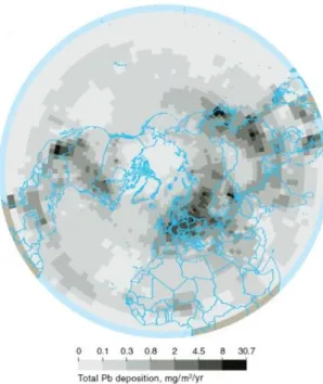
Arctic” (Halbach et al., 2017 adapted from AMAP, 2005). The third AMAP report converged Hg only and emphasized the risks to Arctic ecosystems and humans, as levels of this element are still in-creasing in some regions (AMAP, 2011). Data included in the re-ports was derived from measure-ments of a variety of different ecosystem compartments: the at-mosphere, snow and ice, soils, waterbodies, and flora and fauna. Modeling efforts were specifi-cally focused on atmospheric dis-tribution of metal concentrations as well as their deposition across the Arctic (e.g. Fig. 5, deposition of lead).
In general, levels of metals found in water bodies and soils in the Arctic decreased over the last decades. How-ever, compared to global background levels, atmospheric concentrations of metals are still high near anthropogenic point sources such as mines, smelters and locations of oil and gas extraction (AMAP, 2005). Examples of contaminated environments with elevated metal concentrations are the Pasvik watercourse in the border area between Finland, Norway and Russia, which is strongly affected my nearby smelters (Amundsen et al., 2011), as well as snow in the proximity of the ‘Severonikel’ in-dustrial complex in northwest Russia (Kashulina et al., 2014).
During spring thaw, particulate metals deposited from the atmosphere into the winter snowpack can be transferred to adjacent water bodies in a matter of days to weeks, where they may become available to aquatic biota, such as fish and water-fowl. These important subsistence foods, as well as larger apex predators such as bears, whales and seals, have been shown to be the major pathway of human uptake of metals in the Arctic, especially affecting the traditional diets of many native groups (AMAP, 2005). An important component in understanding this uptake is the process of bioaccumulation, through which even trace amount of metals can build up in both human and animal tissue over time, as well as biomagnification, the in-crease in concentration of a pollutant as it moves to higher trophic levels of a food chain or food web (Van der Hoop, 2013; Datz and Perry, 2012). The most suscepti-ble and vulnerasuscepti-ble group of northern societies are unborn and new-born babies, who
Figure 5. Total annual deposition of lead to the Arctic in 1990, as calculated by the MSC-E Hemispheric Model (Meteorological Synthesising Centre, Moscow) (AMAP,
are at risk of exposure mainly through their mother's diets (Bose-O’Reilly et al. 2010).
In general, both environmental and health effects of metals depend upon on their mobility through environmental compartments (e.g., solubility in water, volatility in air), the pathways through which the metals reach the human body, and the level and time of exposure to the respective contaminant (AMAP, 1998). Yet, the degree of concern for ecosystems and humans varies strongly with each metal. While some are clearly toxic, others are essential micronutrients to the human body but never-theless toxic in excess. Of specific concern are As, Cd, Pb, Hg. These metals, once deposited, can form harmful organic complexes like organolead or methylmercury in the environment, which may cause neurological damage, even at low concentra-tions (Dinis & Fiurza, 2010). Metals such as Cu, Cr, Ni, and Zn, on the other hand, are essential micronutrients for many living organisms, becoming toxic only in ex-cess (AMAP, 1998).
2.4 Carbonaceous aerosols in northern regions
A large fraction of atmospheric particulate matter consists in carbonaceous (i.e., carbon-rich) particles, hereafter abbreviated "CP". These are closely monitored by the air pollution, respiratory health and climate research communities (Petzold et al., 2013). Atmospheric CP strongly absorb visible and near-ultraviolet light, which leads to atmospheric warming (Bond et al., 2013). Furthermore, when deposited, these aerosols lower the albedo of the otherwise highly reflective snow cover (Doherty et al., 2010). This change in the surface energy budget can lead to earlier snowmelt and snow cover retreat, creating a positive snow-albedo feedback that en-hances surface atmospheric warming in the springtime. Next to rising global air temperatures caused by the enhanced greenhouse effect, CPs are considered one of the main drivers for accelerating snow cover decline in the Arctic (Dou & Xiao, 2016).
To account for the wide compositional variety of CP, researchers have developed a multitude of instruments to quantify and/or characterize them (Lack et al., 2013). This can be done based on the chemical composition, optical properties, sources, and morphological characteristics of CP. Definitions and terminology for CP vary with the field of study and analytical techniques (Hegg et al., 2009). A full discus-sion can be found in Lack et al., 2013, Petzold et al. 2013, or Andreae & Gelencsér, 2006. The generic expression black carbon (BC) is broadly used to describe those types of CP that strongly absorb light (Lack et al., 2013; Petzold et al., 2013). The expression thus refers to both their optical and chemical properties. The main source of BC is the incomplete combustion of fossil fuels or biomass (Hegg et al., 2009).
In this work, three different operationally-defined expressions will be used to char-acterize CP filtered from melted snow samples, depending on the analytical method used: elemental carbon (EC), organic carbon (OC), equivalent black carbon (BCe), or effective black carbon (eBC). Briefly, EC (often used interchangeably with BC) and OC are the refractory and volatile fractions of CP, respectively, quantified using the Thermal-Optical Transmittance (TOT) method (Petzold et al., 2013). Their sum is called total carbon (TC). BCe is measured by analytical methods based on light absorption. For the present study, this includes the Particle Soot Absorption Pho-tometer (PSAP; Sharma et al., 2002). The Light Absorption Heating Method, a ther-mal method, quantifies CP in eBC (LAHM; Schmitt, 2019). In the latter two cases, the estimated carbon content might not be BC only, but it is reported as the equiva-lent/ effective quantity of BC that would have the same light absorbance as meas-ured in the sample (Petzold et al., 2013).
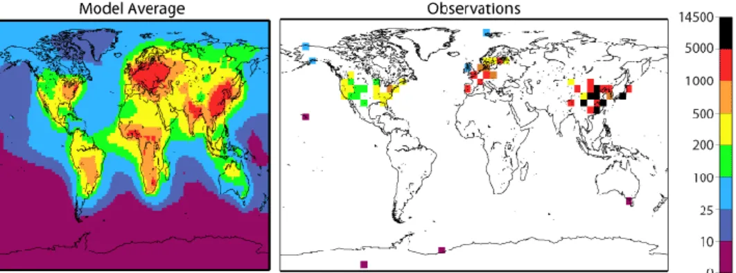
There are several global BC models, that give insight into atmospheric BC con-centrations in the Arctic. As an example, figure 6 shows the average values of sur-face concentration of BC derived from averaging the output of 17 models provided by an aerosol model intercomparison group known as ‘AeroCom’ (Koch et al., 2009). It shows that the atmospheric BC concentrations in the western and central Arctic and subarctic (Alaska, Canada, Greenland) are relatively low with atmos-pheric BC ranging from approximately 10-25 ng/m3 in north-eastern Canada and
Greenland to up to 100 ng/m3 in Alaska and large parts of Canada. Except for the
European High-Arctic (Svalbard; 25-100 ng/m3), the European Arctic and subarctic
experience high BC surface values of up to 500 ng/m3, according to the model mean.
Yet, the study by Koch et al. (2009) found that these models tend to underestimate BC in the Arctic region.
Figure 6. Surface concentration of black carbon for average of AeroCom models (left) and observa-tions (right). Units of the scale are ng/m3 (Koch, 2009).
BC counts as a ‘short-lived climate pollutant’ (SLCP) meaning that these par-ticles remain airborne from a few days to up to a decade, unlike CO2, which can last
for centuries (Schoolmeester et al., 2019). Thus, close emission sources of BC have the greatest potential to impact the Arctic and the subarctic. Comparing the map of global SLCP emission hotspots (Fig. A.1) can therefore explain the above descrip-tion of the modeled atmospheric BC levels. Both biomass burning and industrial emissions in the mid-latitudes of Asia, North America and Europe are driving BC levels. However, the level of emission is highest in Europe and China, which leads to higher contamination levels in the European and Russian high-latitudes.
Efforts to compile information from field measurements were made in the mid-80s (Clarke & Noone, 1985) as well as in recent years (Doherty et al., 2010; Dou & Xiao, 2016). A first survey of CPs in Arctic snow has been undertaken by Clarke and Noone in 1983-1984 (Clarke and Noone, 1985). The two researchers collected 60 samples in the western circumpolar north in order to give a better understanding of the spatial distribution as well as the properties of CP in snow. Several other studies followed, with extensive sampling campaigns during 2005 -2009, which also included taking measurements in the Russian Arctic and subarctic region and the Arctic Ocean (Doherty et al., 2010). Overall, more than 1600 samples were taken, 1200 of which were included in the paper by Doherty et al. (2010) (Fig. 7a)). A follow up has been published by Dou and Xiao in 2016, which included additional measurements from Scandinavia and the European Arctic as well as the Canadian Basin and the Arctic Ocean.
Most of the over 1200 data points included in the dataset were collected in re-mote areas with as little human influence as possible (Forsström et al., 2013; Doherty et al., 2010). An exception was Russia, where a significant portion of the samples could only be taken in areas close to human settlements that were suspected to experience anthropogenic influence (Doherty et al., 2010). Despite the Russian snow sampling locations, the large-scale trend of CP in the snow in remote areas in the high latitudes followed model findings which suggest that the concentration of BC in snow is largely caused by long-range atmospheric transport of particles from lower latitudes (Jiao et al., 2014). According to Dou and Xiao (2016), BC in snow indeed decreases significantly with higher latitudes due to the increasing distance to human activity areas. According to their study, the mean BC concentrations north of 65°N were 13.6 ng/g (Fig. 7b).
Dou & Xiao (2016) clustered the samples from the previously mentioned field campaigns into geographic groups and compared their mean CP values, which showed, that general spatial patterns could be established: With mean BC (termi-nology changes between the different studies, however Dou & Xiao, 2016 chose to use the term ‘BC’) values of 33.7 ng/g and 21.4 ng/g, Western and Eastern Russia
region with mean EC values of 7.9 ng/g. The lowest concentrations were found in snowpacks in the Arctic Ocean (~4.5 ng/g), Western and Eastern Svalbard (~2.5 ng/g and ~7 ng/g), and Greenland (~3.8 ng/g) (Dou & Xiao, 2016). The studies these values are based on measured ‘BC’ and ‘EC’ with different instruments (Doherty et al., 2010: ISSW integrating-sandwich spectrophotometer; Forsström et al., 2013: TOT thermal-optical transmittance) and used different sampling techniques such as surface or bulk sampling. For site specific observation results see Dou et al., 2012, Forsström et al., 2013; and Doherty et al. 2010.
Figure 7. a) All snow-sampling locations used in the paper by Doherty et al. 2010. Colours indicate the different field campaigns on which snow was sampled. b) The variation of BC concentration in snow and ice in spring with latitude. The BC values are derived from the same field campaigns as
described in Doherty et al., 2010 (a) (Dou & Xiao, 2016). b)
As can be seen in figure 7a, published data on snowpacks in the Scandinavian Arctic and subarctic regions are rather sparse. Clarke and Noone (1985) published the first values taken in Abisko, and Forsström et al. (2013) reported measurements from Abisko and Storglaciären, a glacier by Tarfala and the area around Tarfala in Northern Sweden which is at a similar latitude as Kiruna and about 60 km west from the city. The two snow surface sampling campaigns from Storglaciären/ Tarfala in the latter study were carried out in July 2008 (1), and from December 2008 to April 2009 (2) with nine samples taken at three subsites during the first and 15 samples taken at six subsites during the second campaign. The median EC concentration and the 25% to 75% Percentile of campaign 1) were: EC: 42.9 ng/g (range: 42.5–60.5 ng/g) (lat: 67.93) and of campaign 2) 14.5 ng/g (range: 4.0–32.5 ng/g) (lat: 67.91). The two sample locations were reported to have been affected by pollution from local sources. The two campaigns in Abisko were carried out from January to April 2008 with 19 samples taken at 15 forested subsites and the second campaign was undertaken during November 2008 to April 2009: The median EC concentration for the first campaign in Abisko was reported as 51.4 ng/g (range: 27.6–90.7 ng/g) (lat: 68.35) and as 32.2 ng/g (range: 17.5–41.8 ng/g) (lat: 68.35) from the second cam-paign.
3.1 Environmental Contamination and Pollution
The terms ‘environmental contamination’ and ‘environmental pollution’ are often used interchangeably. Contamination, however, defines the “presence of a sub-stance [or energy] where it should not be or at concentrations above background” (Reinardy, 2018 after Chapman, 2007, p.492). Pollution, on the other hand, is a re-sult of contamination (Reinardy, 2018). Chapman (2007, p.492) defines pollution as “contamination that causes adverse biological effects in the natural environment” and Reinardy (2018) adds, that the contamination could be either by natural or arti-ficial means. Thus, pollutants are by definition contaminants, but not all contami-nants become pollutants (Chapman, 2007). Differentiating the two terms is of im-portance to this study, as the exceedance of certain elements above background lev-els can be harmful to people and the environment. In this context, Arctic contami-nation presents a risk to humans, animals and ecosystems depending on the bioa-vailability of specific elements to organisms, the reactions of these elements within the environmental compartment they occupy, and especially the exposure of organ-isms to the respective contaminant (Chemsec, 2016).
3.2
Trace or ‘Heavy’ Metals
The International Union of Pure and Applied Chemistry (IUPAC) has found no less than 38 definitions for ‘heavy metals’, many of which are contradictory (Duffus, 2002). Ranging from “metals with an atomic weight greater than sodium that form soaps on reaction with fatty acids” to “a metal of high specific gravity; esp: a metal having a specific gravity of 5.0 or over” (Hawkes, 1997, p.1374), these definitions use a variety of criteria such as atomic weight or numbers, density, chemical behav-iour and properties (ibid). A common feature is the association of ‘heavy metals’
with toxicity and environmental pollution (Duffus, 2002). As Hodson (2004, p.342) however rightly points out, “toxicity is a function of the chemical properties of the element/compound and the biological properties of the organism at risk”, which de-fines toxicity as a function of the dose rather than being an inherent criterion of a specific element. Hence, to avoid any misconceptions about the term, this report will henceforth refer to the set of metals under investigation as trace elements/ met-als or analytes, which, given their abundance, could reach pollution levels and sub-sequently inflict harmful consequences for ecosystems and people living therein.
The snowpacks of two regions were under investigation: Northern Sweden and the Interior of Alaska, USA (Fig. 8 and 13). The characteristics of these two regions that are of particular relevance to the study are presented in the following sections.
4.1 Northern Sweden
4.1.1 Climate
The snow samples for this thesis were collected in Swedish Lapland, Norrbotten, and Västerbotten, between latitudes 63° and 68° N (region framed in figure 8). Four of the eleven sam-ple locations were situated above the Arctic circle. The climate of this part of Sweden is defined as sub-arctic or arctic (ET = tundra climate according to the Köppen Geiger classification). One important factor influencing the regional climate is the relative position of the Polar Front, which determines whether the dominant air masses originate from the mid-latitudes or the Arctic (CMMAP, N.d). A second factor is the region’s topog-raphy (Fig. 9a). From west to east, the surface elevation drops from ~2500 m. a.s.l in the Scandinavian Mountains (Scandes) down to the northeast coast of the Gulf of Bothnia. The study region lies in the lee of the mountains, which limits precipita-tion rates as westerly winds force moist air from the Atlantic to rise, creating orographic precipitation over the western side of the Scandes (Fig. 9b). Hence, only the western regions of Swedish Lapland profit from these orographic rain- and snow falls, resulting in cumulative precipitation >
4
Study Area
Figure 8: Map of Sweden with sample region marked with a black box.
1900 mm a-1. Regional precipitation patterns are otherwise variable, and sudden, high precipitation events can accompany the passage of low-pressure systems (SCCV, 2007). A third major factor is the heat supplied by the North Atlantic Cur-rent, which results in relatively mild temperatures across northern Fennoscandia compared to other regions at the same latitudes (Fig. 9c) (Palter, 2015). Average annual temperatures are higher at the coast (~4°C) than in the mountains (~-3°C) (Fig. 9c), ensuring a lasting snow cover in higher altitudes throughout the winter (SMHI, 2019c).
Figure 9. Thematic maps of Northern Sweden. a) Topography (GinkoMap project, Nd.), b) annual average precipitation for 1990 (SMHI, 2019b) c) normal annual average temperature for
1961-1990 (SMHI, 2019c).
4.1.2 Snow Conditions
Northern Sweden is entirely covered with snow for almost six months of the year (Fig. 10a), however the depth and duration of snow cover vary across the region depending on factors such as local temperature, topography and predominant winds (Sandström, Nd.).
Figure 10. Climate maps illustrating a) mean for the number of days with snow cover per year for 1961-1990 (SMHI, 2017) b) mean of the largest snow depth during the winter for 1961-1990 (SMHI,
2017a) c): mean for the last day with snow cover for 1961-1990 (SMHI, 2017 b).
a) b) c)
Both snow cover depth and duration decrease towards the south-east and average 175 days per year and 70 cm at the Bothnian coast, respectively (SMHI, 2017). Snow cover can persist until the beginning of June in the Scandes, but only until late April at the coast (Fig. 10c). The snow cover period in most of Sweden has consid-erably shortened within the last decades, but this trend is not yet apparent in the study region (SMHI, 2018). In the 2016-17 winter, maximum snow depth for most of Northern Sweden were recorded on the last day of March (Fig. 11a). The snow samples obtained for this study were collected between 2-9 April 2017. As figure 11b shows, snowpack depths on these days were only slightly less than the late March maxima.
Figure 11. Snow depth in Northern Sweden a) on 31.03.2017 b) on 06.04.2017 (SMHI, 2019d).
4.1.3 Surficial Materials and Soil Chemistry
Sweden has been subject to multiple periods of glaciation and deglaciation, and the most commonly found soil types are those developed from till, covering 75 % of the landscape (Peterson, 2016). Topsoils in the study area are predominantly alpine zols and lithosols, and in Lapland consist mostly in orthic (gleyic and humic) pod-zols (Troedsson & Wiberg 1986). The chemical composition of mineral soils across Sweden has been mapped by the Department of Soil and Environment and the Swe-dish Environmental Protection Agency (Stendahl, 2019). In this study, these maps were used to extract data on major and minor metal concentrations in soil at a depth of 50 cm, near the snow sampling locations.
4.1.4 Pollution Sources: Local and Global
Air
quality in Northern Sweden is high compared to most of Europe, with generally low levels of ambient particulate matter (EU daily limit value: PM10 – 50 µg/m3;PM2.5 – 50 µg/m3 annual limit: PM10 – 40 µg/m3; PM2.5 – 25 µg/m3) (EEA, 2018;
Hak et al., 2009). Modelled annual background PM2.5 and PM10 levels for the last
years were, on average, < 5 µg/m3 across the study region, but they increase towards
the south with the highest concentrations found around Umeå, where they reach 6-8 µg/m3 for PM
2.5 and ~10 µg/m3 for PM10(Willers et al., 2013; Hak et al., 2009).
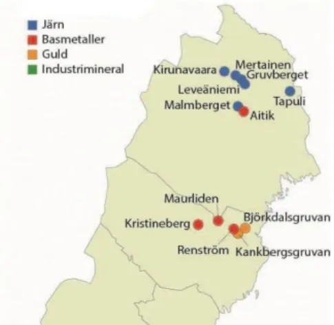
Potential local sources of contaminants include particulate emissions from oil and gas combustion, or from firewood used for residential heating (e.g., Krecl et al., 2008), especially around main population centres. Several large mines can also con-tribute PM emissions from heavy vehicle traffic as well as aeolian dispersion of fine mineral particles from exposed soil and bedrock (e.g., waste rock piles, tailings). The Kiruna iron (Fe) mine in northern Lapland is the world’s largest underground Fe-ore mine. Aitik, just 20 km south of Gällivare, is Europe’s largest open-pit cop-per (Cu) mine as well as the country’s largest gold (Au) producer, and five large Au and base metal mines are an important economic driver for Västerbotten (Fig. 12) (SGU, 2018).
Figure 12. Mines in Northern Sweden in 2018. Järn = Fe, basmetaller = base metals, guld = gold, in-dustrimineral = industrial minerals (SGU, 2018).
Apart from local contamination sources, the snow cover in Northern Sweden may also collect aerosols delivered by long-range atmospheric transport from dis-tant sources. The widespread acidification of forests and lakes in the 1960s-70s made it clear that Sweden is exposed to contaminants introduced to the region by air masses moving across industrial regions elsewhere in Europe or beyond (Maas & Grennfelt/ UNECE, 2016). A study conducted by the European Environmental Agency (EEA) in 2013 names Germany, Poland, Denmark, Great Britain and Nor-way as the five highest foreign emitter countries in terms of primary and secondary PM2.5 emissions affecting Sweden (EEA, 2013).
4.2 Interior Alaska
4.2.1 Climate
Snow samples used in this study were obtained in Interior Alaska, which is commonly defined as the region between the Alaska Range to the south, the Brooks Range to the north, the Canadian border to the east, and the southwestern flats to the west (ADF&G, N.d.; Shulski & Wendler, 2007). The study area is lo-cated in the eastern part of Interior Alaska (region framed in figure 13), and all samples were collected between lati-tudes 63°N and 65°N, below the Arctic Circle. The dominant feature of Interior Alaska’s climate is its continentality, owing to its remoteness from moderating coastal influences. Large interseasonal temperature variations (-62° to 38°C), low humidity, and low and irregular precipi-tation rates define the region (Shulski & Wendler, 2007). Temperatures in winter can drop well below -40°C, especially in valleys and depressions, although long periods of extremely cold temperatures have become less prevalent over the last decades (Stuefer, 2019). The relationship between temperature and latitude (Fig. 14) is more expressed in winter than in summer.
Figure 14. Mean Annual Temperature in Alaska (°C) (Walsh/ AK CASC, 2018). Figure 13. Map of Alaska with sample region
The main climate control during the winter is a prevailing high-pressure system. This changes in summer, allowing warm, moist air from lower latitudes to come into the region (Shulski & Wendler, 2007). Prevailing winds during the cold season months (Sept.-May) are from the north, switching to southerly winds in the summer months (June-Aug.). Due to the high-pressure system in winter, surface wind speeds are usually low, which can lead to strong temperature inversions in certain locations such as Fairbanks. Occasionally, low-pressure systems track through Interior Alaska during winter months, often associated with snowfall. Anticyclones with surface pressures ≥ 1030 mb have also been observed to move into as well as form in the Interior, which oftentimes leads to extremely low temperatures (ibid).
Most of the annual precipitation in Interior Alaska falls during the summer months as rain, except for the high mountain ranges, where solid precipitation pre-dominates (Fig. 15; Shulski & Wendler, 2009). Within the study area, mean annual precipitation varies from 200 mm in low-lying areas such as the Tanana-Kusko-kwim Lowlands (~200-900 m.a.s.l.), to 700 mm in the foothills of the Alaska range (> 900 m.a.s.l.) (Fig. 16).
Figure 15. Downscaled projections of rain/snow partitioning for Alaska shown as Snow-day Fraction (%). Blue shades indicate high snow to precipitation ratio, green shades indicate less solid
4.2.2 Surficial Materials and Soil Geochemistry
The topsoils of eastern Interior Alaska are dominated by gelisols (turbels) and in-ceptisols (aquepts, gelepts, and cryepts). Gelisols are soils that are frozen for a part of the year and contain permafrost near the surface. Turbels occur mostly in places that receive enough solar radiation for the top layer to thaw in the summer months, or in areas that have been subject to forest fires or land clearing (USDA/NRCS, N.d.). Inceptisols are very poorly developed soils mostly situated in wet areas with a deeper active layer than Gelisols or no permafrost at all (USDA, 1999). Soils of the Tanana series, which are aquiturbels developed from loess or alluvium in per-mafrost areas, are prevalent in the interior of Alaska (Mulligan& Cole, Nd.). Chem-ical composition maps of the topsoils in Alaska have been compiled by the U.S. Geological Survey (USGS) based on soil and sediment measurements taken since the 1960s by the USGS, the National Uranium Resource Evaluation program, and the Alaska Division of Geological & Geophysical Surveys geochemical databases (Lee et al., 2016). In this work, the USGS maps were used to extract information on metal concentrations in soils in proximity of the snow sampling locations.
4.2.3 Snow Conditions
The duration of snow cover across the study region varies considerably with alti-tude. Low-lying areas such as the Tanana-Kuskokwim Lowlands experience 170-210 days of snow cover every year while in higher areas such as the Yukon-Tanana Uplands and the Steese National Recreation Area (SNRA) it may last 210-260 days, or 250-290 days near the Alaska Range (Lindsay et al., 2015; data for 2001-2013). This pattern is mirrored by mean annual snow water equivalent (SWE; Fig. 17), which decreases from >40 cm in the foothills of the Alaska Range to >10 cm in the Tanana-Kuskokwim Lowlands. The last day of snow cover in Interior Alaska also strongly varies with altitude (Fig. 18). The snow may disappear in early April in the Tanana flats but can persist until the beginning of June in parts of the Yukon-Tanana Uplands and the foothills of the Alaska range. For the winter 2017-18, when the snow samples for this study were taken, the study region experienced above-average winter snow accumulation. On May 7, 2018 (start of the sampling period), the snow now depth across the study region was ~15cm greater than to the average for 1998-2012 time period. The contributing factors were both colder than average winter and spring air temperatures, and above-average winter precipitation (Brown & Luojus, 2018).