The Euro Effect on Trade
The Trade Effect of the Euro on non-EMU and EMU Members
Bachelor’s thesis within Economics
Authors: Ga Eun Choi
Stephanie Galonja
Tutors: Pär Sjölander
Peter Warda Jönköping December, 2012
Bachelor’s Thesis in Economics
Title: The Euro Effect on Trade: The Trade Effect of the Euro on non-EMU and non-EMU members
Author: Stephanie Galonja and Ga Eun Choi
Tutor: Pär Sjölander
Peter Warda
Date: 2012-12-18
Keywords: EMU, Gravity model, the European Union, Bilateral trade, Panel Data, Random Effects Model
Abstract
The purpose of this paper is to investigate how the changes in trade values are affected by the implementation of the euro currency. We study the EU members, including 11 EMU members and 3 non-EMU members (Sweden, Denmark and the United Kingdom). The empirical analysis is conducted by using a modified version of the standard gravity model. Our core findings can be summarized into two parts. First, the euro effect on trade which is estimated by the euro-dummy coefficient reflects an adverse influence by the euro creation on trade values for the first two years of the implementation on all our sample countries. It leads us to a conclusion that there is no significant improvement of trade in the year of implementation. These results do not change when a time trend variable is added to evaluate the robustness of the model. Our primary interpretation is that the euro creation does not have an immediate impact on trade but it is rather gradual as countries need time to adapt to a new currency. It is connected to our second finding that the negative influence of the euro implementation is not permanent but eventually initiates positive outcomes on trade values over time, thus concluding that the euro implementation has had gradual impact on both EMU and non-EMU members.
Table of Contents
1. Introduction ... 3
1.1 Purpose ... 4
1.2 Delimitations ... 4
1.3 Outline and Frameworks ... 4
2. Background ... 6
2.1 The European Market Integration ... 6
2.2 Sweden, Denmark, United Kingdom and the EMU ... 7
3. Previous Studies ... 9
4. Theoretical Frameworks ... 11
4.1 The Optimum Currency Area Theory ... 11
4.2 The Gravity Model ... 12
4.3 The Random Effects Model (REM) ... 13
5. Empirical Frameworks ... 15
5.1 Data ... 15
5.2 Empirical Model and Variables ... 16
5.3 Descriptive Statistics ... 17
6. Empirical Analysis ... 20
6.1 The Euro Effect on Trade ... 20
6.2 Diagnostic Tests ... 24
6.3 The Euro Effect on Trade with Time Trend Variable ... 26
6.4 The Rise of the Euro Effect... 29
7. Conclusions ... 31
7.1 Suggestions for further studies ... 32
List of References ... 34
Appendix 1: Summary of previous research ... 37
Table A1 Summary of Previous Research for Further Reading………….. ... 37
Appendix 2: GDP graph for sample countries ... 38
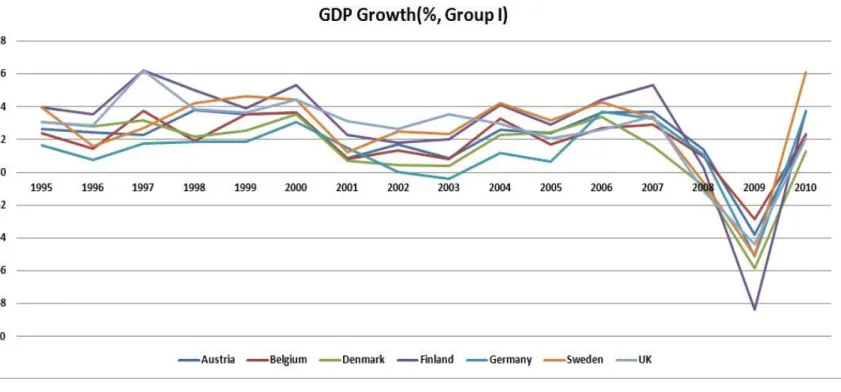
Figure A 2.1 Real GDP Growth Rate (Group 1) from 1995 – 2010 ... 38
Figure A 2.2 Real GDP Growth Rate (Group 2) from 1995 – 2010 ... 39
Appendix 3: Test result ... 39
Table A 3.1 Descriptive Statistics GDP ... 39
Table A 3.2 Descriptive Statistics for Sweden’s Total Trade Value ... 39
Table A 3.3 Descriptive Statistics for Sweden’s Logged Total Trade Value ... 40
Table A 3.4 Descriptive Statistics for Denmark’s Logged Total Trade Value ... 40
Table A 3.5 Descriptive Statistics for United Kingdom’s Logged Total Trade Value……….. ... 41
Table A 3.6 Descriptive Statistics for Dummy Variables ... 41
Appendix 4: Eviews Ouput Adjusted for the Time Trend ... 42
Table A 4.1 Robustness Test for Sweden ... 42
Table A 4.2 Robustness Test for Denmark ... 42
Table A 4.3 Robustness Test for the United Kingdom ... 43
Table A 4.4 Robustness Test for the EMU countries ... 43
Appendix 5: Figures for Residual Normality Tests ... 44
Figure 5.1 Histogram for Sweden ... 44
Figure 5.2 Historgram for Denmark ... 44
Figure 5.3 Histogram for the UK ... 45
1. Introduction
The impact of the European Monetary Union (EMU) on trade has always been the center of dispute as it is an inevitably crucial aspect in discussing the actual gain of joining. The impacts of common currency unions are expected to be positive according to previous studies, as it is known to provide a platform for optimum base for free trade by removing uncertainty factors such as exchange rate volatility. However, if we perceive EMU as a process of implementing the euro currency, what is its merit to non-EMU members who are already protected under the free trade agreement of the European Union (EU)1 as well as the EEA agreement? Has EMU really upgraded the market integration concerning trade to a different level than the frameworks of the EU?
This investigation focuses on the impact of the euro currency on trade between EMU and non-EMU members within the European Union (EU). We use a standard gravity model to run panel data analysis on a total of 14 countries, where 11 are EMU members and 3 are non-EMU members, namely Sweden, Denmark and the United Kingdom, in the years 1995 to 2010. We observe trade patterns between the countries to find a relation between the implementation of the euro and trade values. We study two main research questions. First, we answer the question of whether the creation of the euro does or does not improve trade. Second, construct an analysis on which year the euro effect shows significant changes.
In contrast to earlier research, we make two unique contributions. We use the most recent data available which will end and include the year of 2010. The extended time span will allow us to reflect the current European economic crisis on intra-European trade. However, it is also a source of limitation as the crisis will cause unusual trade patterns that are not related to the creation of EMU. Moreover, we compare our original empirical model to a new model with a time trend variable in order to remedy a potential deterministic trend and show why some of the previous studies might have had inflated estimates on the euro effect on trade.
The previous research on the euro effect2 varies in great detail as different models and time periods are used. Some of the articles introduce the euro as an ultimate trade booster whereasothers reasonably argue the opposite (Rose, 2000; Barr, 2003; Bun and Klaassen, 2007; Baldwin, 2006). EMU (We use EMU, the euro currency area and Eurozone interchangeably) aims to reduce exchange rate volatility and transaction costs3 through the European market integration. Many of the earlier studies estimate that the euro currency union will significantly increase the trade values of its member’s states thus promote labor movement and market expansion. However, it is ambiguous whether the benefits of the market expansion exceed the macroeconomic costs of joining the Eurozone. Consequently losing control over an economy’s monetary policy. Bun and
1 The reader should be cautious that when we refer to the ’free trade agreement’ we do not specifically
mean the European Free Trade Agreement (EFTA). In the thesis, the free trade agreements refer to the former treaty clauses that provided the fundamentals of EMU such as the ’Treaty of Rome’ and the ’Treaty of the European Union’.
2 As it has been mentioned in the abstract, we define the euro effect as the changes in trade values caused
by the creation of the euro currency.
3 Transaction cost in our research is defined as the cost incurred when adjusting exchange rate in order to
Klaassen (2007) even argue that when a time trend variable is included and deterministic trend is removed, the return from the euro implementation is smaller than what many researchers have predicted. This type of investigation is rather important for Sweden, Denmark and the United Kingdom, as they are members of the EU but have not yet joined the third stage of EMU. In fact, these countries are already protected by the trade customs of the EU which has been established many years prior to the implementation of EMU. The EU as an extensive form of a supranational union has successively pursued the higher level of financial market integration and without any doubt the euro became the potential leading currency of the world. However, joining EMU is still a question to be answered seeing the current economic crisis in Europe.
1.1
Purpose
The purpose of our research is to investigate the euro effect which is defined as the changes in trade values caused by the implementation of the euro currency in 1999. The study explores whether there has been any significant impact of the implementation of EMU and when this effect arises.
1.2
Delimitations
The length of the time span in the dataset may be a potential weakness of the study. However, due to data accessibility reasons, the sample period could not have been prolonged in any direction. Also, we have chosen to use the random-effects model because our gravity model includes time-invariant variables whereas the fixed effects model only allows time-varying variables. Thus, even if a Hausman test would recommend a fixed-effects model, it would not be possible to estimate this model since the time-invariant variables would cause perfect multicollinearity. Furthermore, the analysis on the delayed euro effects which we try to investigate by lagging the year of implementation can be further improved. It is difficult to capture the full effects of a change through this method.
1.3
Outline and Frameworks
In panel data frameworks, we run a regression on the amount of total trade values. We use a standard gravity model which consists of two variables such as GDP of two countries engaged in trade and the distance between them. We add two dummy variables, one time variant dummy for the creation of the euro and one time invariant dummy for co-founder countries of the first free trade agreement among the European nations, the European Economic Community. We add this variable to investigate whether being engaged in a free trade agreement earlier than other members is more beneficial and what role it will play in trade.
Furthermore, the limited number of time periods in the sample which is from 1995 to 2010, can unintentionally influence trade values and GDP due to suffering from the European sovereign debt crisis over the last few years. The reason as to for why we use data from 1995 to 2010 is solely due to data accessibility reasons.
In Section 2, we will provide the readers with necessary background knowledge concerning the free trade agreements between the members of the EU. As we believe that the increase in current trade value is partly due to the former treaties such as the ‘Treaty of Paris’ and the ‘Treaty of Rome’. In Section 3, we will discuss previous studies that are relevant to our topic. In the theoretical frameworks, presented in Section 4, we will explain the optimum currency area theory and the gravity model, providing support for our results. Lastly, in Section 5, we will present our modified version of the gravity model with data analysis where we will draw conclusions, providing insights on the previously mentioned research questions. Moreover, suggestions for further studies will be given on this topic.
2. Background
The European Monetary Union (EMU) should be viewed as a process of creating an optimum currency area within the European Union, through financial and labor market integration. EMU is mainly composed of three stages where the first two stages involve pegging domestic exchange rates according to a proposed level and meeting the requirements of EMU followed by the third stage of the actual implementation of the euro. The main objective of EMU is to increase trade through market integration and reduced exchange volatility risks (Berger and Nitsch, 2005). In 1999, 11 countries joined and as of 2007, a total of 17 member states4 entered EMU. Despite the fact that the euro was implemented in 1999, the development of the free trade agreement among the member nations of the EU began prior to the euro creation under former treaties. In this section we briefly discuss these former treaties as we include a treaty dummy in the empirical model later presented in this paper.
2.1
The European Market Integration
The common conclusion in previous studies is that the creation of the euro does have a positive impact on trade to a certain extent. However, it is difficult to view the current upward trend in trade to simply be a result of the euro. That is why it is important to study the history of the European market integration in order to acknowledge other historical impacts on the current increase in the internal and external trade of the European Union. For the purpose of this paper we focus mainly on the economical (industrial) integration rather than the political aspects. In this section, we give an overview of the three most important treaties, the ‘Treaty of Paris’ in 1951, the ‘Treaty of Rome’ in 1957 and the ‘Maastricht Treaty’ in 1992.
The Treaty of Paris, also known as the European Coal and Steel Community (ECSC) was established in 1951. It was the first industry related treaty that included Italy, West Germany, France, Belgium, Luxembourg and the Netherlands, countries referred to as ‘The Inner Six’. The treaty dealt with the production and trade shares of coal and steel (Kitzinger, 1960). ECSC was the first step towards the European Union, as later ‘The Inner Six’ became the founding members of the prior EU communities. (Europa, 2010) Following the ‘Treaty of Paris’ in 1957, the ‘Treaty of Rome’ was signed. It included two very important treaties at the time, the European Economic Community (EEC) treaty and the European Atomic Energy Community. The main objectives of the ‘Treaty of Rome’ were ‘the creation of a general market’ and ‘the creation of an atomic energy community’ (Europa, 2010). Furthermore, it established a custom union under the same trade policy, eliminating tariffs and trade quotas, aiming to increase trade between the EEC (Bartels, 2007).
The expansion of the intra-European market continued over the following years by amending treaties such as the ‘Treaty of Brussels’, also known as the ‘Merger Treaty’ in 1965 and the ‘Maastricht Treaty’ also known as the ‘Treaty of the European Union’ in 1992. These treaties combined ECSC, EEC and the European Atomic Energy
4 Austria (1999), Belgium/Luxembourg (1999), Finland (1999), France (1999), Germany (1999), Ireland
(1999), Italy (1999), Netherlands (1999), Portugal (1999) ,Spain (1999), Greece (2001), Slovenia (2007), Cyprus (2008), Malta (2008), Slovakia (2009) and Estonia (2011).
Community into a single operative system taking a step closer to their objectives of the European market expansion.
The current trade clauses of the EU are constructed in detailed manners with the well-organized platform of the former treaties. These treaty clauses can be summarized into the three key words; free, fair and extended market (Europa, 2010). The Treaty of Rome, clearly states that the member nations should eliminate trade obstacles ‘in order to guarantee steady expansion, balanced trade and fair competition’. Along with ‘measures common with the custom tariffs, the removal of custom duties and of quantitative restrictions on impact and export of good, and the ‘Treaty of Rome’ eliminated trade customs. (The Treaty of Rome article 3 (a), p. 4)
Therefore, the creation of EMU should not be perceived as a radical change of the European market system but as an extension of these treaties. It is evident that the former treaties have provided the basics of the market integration and that the current trade relations between the EU members are accumulated impacts of these treaties. The ‘Treaty of the European Union’ concludes all the former treaties into three stages, providing the pillars of EMU (European Comission, 2011):
1. Incorporate the European capital market into one by December 31st, 1993. 2. Introduce the European Monetary Institute (EMI) and establish the European
Central Bank (ECB) in order to unify economic policies among the Central Banks of the member states by December 31st, 1998.
3. Adapt the euro as the single currency between the member states under the joint monetary policy of the European Central Bank (ECB) by December 31st, 1998. This stage is yet to be completed since only 17 out of 27 members of the EU have reached this stage(European Comission, 2011).
All member states of the EU are now assigned to join the third stage of EMU. However, a few countries such as Sweden, Denmark and the United Kingdom are pending their decisions to enter due to structural and political aspects of their economies.
In short, the previous treaties have not reached the level of the currency union; however their efforts of unifying trade policies are reflected in the trade value changes.
2.2 Sweden, Denmark, United Kingdom and the EMU
The question of whether the three non-EMU countries under investigation should enter the third stage of EMU has been raised on numerous occasions. The opposing public opinion and lack of credibility of the new currency union are the main aspects of the disputes. In 2003, 55.9% of the Swedish citizens voted against joining EMU5 (Flam and Nordström, 2006).The main reason being the fear of losing the control over its domestic monetary policies. According to the ‘Maastricht Treaty’, every nation in the EU must fulfill the convergence criteria in order to enter EMU. Sweden chose not to participate in the exchange rate mechanism (ERM). However, the recent Swedish recession changed the situation and in 2009 47 % of the Swedish population supported EMU while 45 % were still against it (Grahnlaw, 2009). The Swedish choice of dealing with this matter is to “wait and see” in order to become more acquainted with EMU and its
5
effect (Reade and Volz, 2009). Even though Sweden does not have a direct plan of entering EMU in the foreseeable future, the euro is still a part of the Swedish policy program as they are in the preparatory stage of joining (Flam and Nordström, 2006). In 2011, approximately 56% of the Swedish exports were to the Eurozone, while 69% 6 of the Swedish imports originated from the Eurozone without having joined the EMU. Therefore, the question of joining or not is still a tough decision for Sweden.
Fortunately, for the United Kingdom and Denmark, this matter is less severely discussed as they are not obligated to join the third stage of EMU (Europa, 2006). They hold the rights to join at any time, since they meet the required conditions. Meanwhile the governments of the United Kingdom and Denmark are still in doubt as the expected outcomes are ambiguous.
6
3. Previous Studies
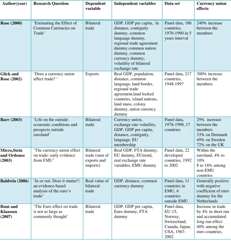
The euro effect on trade has been investigated extensively on the basis of the gravity model. The impact of the common currency union on trade is still controversial on multiple dimensions and the previous estimates on the euro effect vary in great range depending on the model. In this section we present the selected literature relevant for our purpose7.
The gravity model has been used in many previous studies, discussing the relationship between common currency area and trade. Rose (2000) explains in his model that a common currency area greatly improves bilateral trade among the associated countries. He states that in the case of EMU, the expected returns on joining EMU are accounted to be 240% increase in trade which is a relatively high figure compared to other studies regarding the common currency union (Rose, 2000). His remarkably high estimate on the euro effect is often referred to as the ‘Rose effect’ (Rose 2000; Baldwin, 2006). Despite his pioneering work in the field, Rose is criticized on two bases. The first is that his sample countries are mainly developing countries potentially leading to high estimates. The second concerns the ‘endogeneity’ issue. The endogeneity issue arises in two circumstances. Barr (2003) explains that one of the two cases appear when an empirical model omits an important source of trade increase as an explanatory variable thereby the coefficient of another variable such as the trade effect of EMU will be larger since it will indirectly cover the missing variable’s impact. In result, it will lead to higher estimates of a certain independent variable. Rose (2000) tried to overcome this problem by adding all possible variables avoiding the trouble of misspecification, however, his approach is once again criticized by Persson (2001). Persson explains that if some of variables with non-linear relationships with bilateral trade are included as if they do have linear relationships, this will lead to biased estimates as well. Barr (2003) suggests that a possible solution for endogeneity issue is to add fixed effects which can work as a proxy for missing variables. The idea of fixed effects appears in Glick and Rose’s model in 2002 as well. They add ‘fixed country-pair specific intercepts’ in order to capture all time invariant impact on trade (Bun and Klaassen, 2006). This method is actually very useful in reflecting different natures of the sample countries that the model cannot cover.
Barr (2003) uses a modified version of Glick and Rose’s model in his research when investigating the euro effect on non-EMU countries. However, he focuses on the exchange volatility as he believes that the main source of increase in trade will be due to reduced exchange volatility risk. He predicts different returns for Sweden, Denmark and the United Kingdom as the extensiveness of the exchange volatility impact is different for each country. He estimates that Swedish trade would have increased by 49%, Danish trade by 34% and the British trade by 72% if they had joined the union since 2001 (Barr, 2003). For EMU members, the estimate is comparatively lower at 27%. However, he emphasizes that the entry to EMU was not the cause of trade increase but the evolution of trade policies between members encouraged trade between them (Barr 2003).
7 Research that is relevant but does not directly involve the euro currency has been included in the
Micco et. al (2003) suggest that the impact of the creation of a common currency area is not only limited to the member countries, but also worldwide. They estimate the effect of the EMU on bilateral trade to be in the range of 5 % to 10 % between the euro countries whereas the trade impact will vary from 9% to 20% among the non-euro countries. They claim that it is possible for non-EMU members to gain more than the actual members by having one large currency union as a neighbor.
Bun and Klaassen (2006) report that existing gravity models are overestimating the extent of the euro effect on trade. They state that previous researchers present an increase in the trade value of 5% to 40 % and do not take time trend into account. By including a time trend to a gravity model, Bun and Klaassen’s research show that there is only a 3 % economic effect on trade volume caused by the euro (Bun and Klaassen, 2006). Many of the previous researchers omit or overlook the importance of this matter which leads to high estimates of the euro effect on trade. Bun and Klaassen’s method of removing deterministic trend is a fairly new concept and it questions the robustness of previous studies, which will be dealt with later in the empirical analysis.
On the other hand, there are studies with negative values of the expected return on the currency union. Baldwin (2006) gives an interesting result as he opposes earlier studies, suggesting there can be a negative or null coefficient for the euro dummy which can lead to an assumption that the euro creation actually decreases trade among the trade partners. Many of the earlier studies have suggested that the common result of being a member of EMU is increased trade. However, Baldwin reports a negative influence of the euro regarding, for instance, the Dutch exports. In fact, this outcome coincides with Rose’s (2000) earlier remarks, ‘the simple correlation between trade (value) and the common currency dummy is small and negative’ which Rose again explains that the inclusion of other explanatory variables can change the coefficient of the euro dummy into a positive figure (Rose, 2000).
Nevertheless, these previous studies suggest that the estimated impact of EMU varies in great sense depending on the model of choice and the number of observations. The estimated returns of a currency union are still ambiguous. For instances, McKenzie (1999) states that “fundamental unresolved ambiguity exists (between exchange rate volatility and trade)” despite the fact that many researchers claim the reduced exchange volatility risks to be the main source of a trade booster.
4. Theoretical Frameworks
In this section we explain the meaning of an optimum currency area and the expected costs and benefits of a currency union. Also the theory behind the gravity model is explained for the further interpretation of the empirical analysis.
4.1
The Optimum Currency Area Theory
Mundell introduced the theory of Optimum Currency Area (OCA) in 1961 and defined a single currency area “as a domain within which exchange rates are fixed” with “a single central bank (with note-issuing powers)’’ (Mundell, 1961, p. 657). The known effect of pegging a currency to a single fixed currency is the reduced risk of fluctuations and economic imbalance (Mongelli, 2005).
Frankel and Rose (1996) state that in order to minimize the cost of market integration while increasing the benefits of creating a single currency union, countries should meet the following properties. First, a large volume of bilateral trade between the countries is required. Second, the engaged countries should have similar economic patterns of fluctuations. Third, the mobility of labor should be high in order to maximize the economic outcomes. Lastly, the risks of market integration should be equally shared (Frankel and Rose, 1996). In the case of EMU most of these criteria are met to a large extent.
The benefits of EMU are mainly initiated by two factors such as the reduction of exchange rate volatility risk and transaction costs. According to Frankel and Rose (1996), this will in turn lead to an increased trade among countries as well as an increase in foreign direct investment due to the increased credibility. In fact, the integration of financial markets under a unified currency can go beyond the spectrum of a free trade agreement. Thus, the single currency will gain collective power compared to a situation where each country has its own currency (Mongelli, 2005). Frankel and Rose (1996) state that the highly integrated market will lead to a higher integration level of their business cycles. However, Krugman (1993) and Kenen (1969) suggest the opposite. They suggest that once the countries are economically integrated, they tend to focus on goods with their comparative advantages. In other words, the higher the integration process, the larger the divergence of business cycle (Frankel and Rose, 1996).
However, even though the estimated benefits are larger than the costs, there are also macroeconomic costs involved when creating an optimum currency area. The most obvious cost is the currency changeover. The national governments of the member states must bear the costs of adapting to a new monetary system and also, the extra costs concerning the formation of a unified institution. In addition to this, Feldstein (1997) states that since the different nations are affected by different economic shocks, the single currency will contribute to the difficulties of conducting a unique monetary policy as well as the market’s ability to correct for exogenous shocks. He explains that these limitations in macroeconomic policies will increase cyclical unemployment of the members of the single currency union (Feldstein, 1997). The current economic crisis is a good example of the difficulties of having a supranational union. If one, in this
particular case, Greece, fails to meet the optimum level of economy, others must bear the costs together. The monetary policy involving all countries can rather be a delicate issue.
4.2
The Gravity Model
Tinbergen (1962) and Pöyhönen (1963) are the pioneers of the gravity model explaining bilateral trade between two countries within the frameworks of their economic sizes and the distance between them. The gravity model is a commonly used empirical trade theory model because of its high accuracy in explaining different trade patters between trading pairs.
A simple gravity model shows the relation between bilateral trade between two countries and two explanatory variables such as GDP and distance. It is very often that the GDP per capita is used in order to control GDP according to population. It is generally known that GDP variable is positively correlated to trade whereas distance is negatively correlated to trade. These predictions are rather logical as high GDP, equivalently to large economic size tend to produce more goods and therefore trade more. There are exceptions in certain cases where large economies consume the majority of their production and therefore trade less. However, this case is rather rare in reality. Geographical distance is often very negatively related as longer distance incurs higher transportation costs and other transaction costs. The gravity model is recognized for its easy use as it can include dummy variables according to the purpose of its use. In the early stages of the gravity model, Tinbergen (1962) used GNP and distance as independent variables to explain the volume of trade. It did not include any dummy variables but simply investigated the trade influence of economic sizes and distance. Benedictis and Taglioni (2011) describe Tinbergen’s coefficients of the independent variables as “coefficients of the economic attractors”, as they are presented as the indicators of trade attractiveness of a country (Benedictis and Taglioni, 2011, p. 58). The authors state that the fit of the model increases as the sample size increases. This result can be therefore very largely depending on the sample size.
Equation 1. the original form of the gravity model
The simple gravity model introduced by Tinbergen (1962) contains only two variables, Y and d, which are GDP and the distance between two countries. C in this case is the constant which presents how much change in GDP will be reflected on trade. If we convert Equation 1 into a log-log model, we will have Equation 2. Therefore, if log of C is less than 0, the actual value of C is between 0 and 1 and if log of C is greater than 0 it signifies that the actual value of C is larger than 1. Meaning trade is greatly influenced by the GDP of both countries, ( . Therefore, a negative constant does not necessarily indicate a negative impact on the trade value, but it means that trade is fairly constant despite changes in GDP.
Over the years, modifications were made to the gravity model such as a log-log form, as shown in Equation 2. The log-log form of gravity model is commonly used as it is easy
to analyze the results as they show the elasticity of bilateral trade in percentage. The main variables used in the sample gravity model are the same as the Tinbergen’s gravity model where presents a constant, C. Consequently, is an exporter’s GDP whereas signifies the importer’s GDP. presents the distance between two trading partners
and lastly the error term, , is included to capture omitted influences (Benedictis and L. De, 2011).
( ) ( )
Equation 2. A sample gravity model
The gravity model can be biased, as seen in the case of Tinbergen’s model (1962). One must acknowledge the fact that the constant will vary depending on its trade partners and that the high correlation between variables can lead to a biased result. Even in its basic form, the gravity model contains correlation between variables such as GDP and GDP per capita. If this is not accounted for the gravity model it will present biased results. There have been many attempts to solve this problem by amending for the time trend and using panel data instead of cross-sectional data given the assumption that the panel data will correct for country heterogeneity. Panel data is also known for providing higher reliability when it comes to investigating policy effects furthermore, you can include dummy variables according to your purpose (Benedictis and L. De, 2011). After all, the gravity model is constantly revised by economists and statisticians and is a widely used model in international trade theory.
4.3
The Random Effects Model (REM)
According to Gujarati (2009), a random effects model (REM) does not reflect any individual specific effects on its coefficients estimates. The model assumes that the samples are randomly drawn from its population therefore the samples are uncorrelated with the explanatory variables. Therefore the model does not treat as a fixed intercept but as a random variable with a mean value. The intercept for a sample can be expressed as the following equation:
Equation 3. Intercept in a random effects model
In Equation 3, εi represents a random error term with a mean value of zero and a finite
variance. Hence, the individual differences in the intercept, over each sample are represented by εi.
In order to bring further understanding, the gravity model with a time trend variable is used as an example.
( ) ( ) Equation 4. A sample gravity model with a time trend variable
Substituting Equation 3 into Equation 4, we obtain
=
( )
Where
Equation 5. A sample gravity model with a combined error term
combines two error terms together, namely and . represents the
cross-sectional error and signifies the combined the error of time series and cross-section which varies over individual regression.
In the random effects model, the intercept signifies the mean value of all individual cross sectional intercepts between trading pairs. The error term is provided to overcome the random deviation of the individual intercepts from the mean value. We have used a similar form of the random effects model and the further analysis of its use will be explained later in the analysis section.
5. Empirical Frameworks
In this section we will present our gravity model with the chosen variables and discuss the nature of our empirical studies. The main purpose of this section is to investigate the correlation between the increased values of trade among the core members of the European Union and the creation of the euro. We will discuss what changes the euro effect has initiated for both EMU and non-EMU members.
5.1
Data
For our empirical studies, we conduct a panel analysis with a random effects model for both with and without time trend as a variable, using 14 European countries; 11 EMU members and 3 non-EMU members. We evaluate the time period from 1995 to 2010 due to data accessibility reasons. The periods are divided into before and after the euro creation. We take the years between 1995 and 1998 as our prior to the euro period and from 1999 and onwards as the post euro period. In 1999, 10 countries within our sample joined the third stage of EMU8. All data is presented in annual terms. They are converted into US dollars at current price and current PPP. We use 176 observations in total for the panel data analysis. All the statistical data is retrieved from the OECD stat website and the distances between the trade pairs are calculated on http://www.distancefromto.net/. When we approximate the distance, we simply take the distance between the two countries’ capitals.
We run a panel random effects model as we have multiple time periods with cross sectional data. We analyze 11 cross-sections over the 16 year period which makes a total of 176 observations per non-EMU country. Using the same method, we take 110 cross-sections over the 16 year period for the EMU members. In order to investigate the changes in the euro effect over the years after the implementation, we lag the starting year of EMU for the euro dummy from 1999 and continue lagging until the coefficient of the euro dummy shows positive changes.
Table 5.1 List of sample countries
EMU members (before the 2004 expansion) Non-EMU members
Austria Belgium/Luxembourg9 Finland France Germany Greece Ireland Italy Netherlands Portugal Spain Sweden Denmark United Kingdom 8 Greece joined later in 2001.
9 OECD stat does not provide separate data for Belgium and Luxembourg. Therefore the data presented
5.2
Empirical Model and Variables
We try to recreate Rose’s (2000) earlier form of the gravity model. We make few modifications in accordance to our purpose. We exclude all the ‘colonial dummies10’ as they are irrelevant to our sample countries. Rose’s model is in fact very similar to the basic gravity model, originated from Tinbergen (1962) and Pöyhonen (1963).
The following equation represents our model:
( ) ( ) ( ) +
t is a time index
Equation 6. Empirical gravity model without a time trend variable
Table 5.2 List of Dependent and Independent Variables
Variable Description Coefficient
( ) Dependent variable. Natural logarithm of total trade between
country i and j at time period t in US dollars. Time variant variable.
Constant
( ) Natural logarithm of the overall economic activity of country i and j11 . Y signifies GDP value retrieved from an output approach.
Time variant variable.
( ) Natural logarithm of distance between country i and j (All distances are counted in kilometers)
Time invariant variable.
Euro currency dummy, time variant variable
{
European Economic community dummy, time invariant variable
{
Error term =
10 Rose (2000) include dummies representing colonial relationships such as the ’common nation dummy’,
’colonies under the same colonizers after 1945’. Also, ’if county i colonized j or vice versa’.
11
In our random effects model without time trend, we chose our dependent variable as the log of the total trade between two trading partners. OECD Stat defines the total trade value as the sum of imports and exports. The aggregated amount of both exports and imports will indirectly reflect the changes in exchange rates between trade-pairs (Flam and Nordström, 2006). In our case, all the sample countries are within the European Union; therefore exchange rates cannot be a main source of fluctuations in total trade value. Again, for the purpose of recreating the Rose’s earlier model, we use the same dependent variable as in that of Rose (2000).
We make one variation from the Rose (2000) and Barr’s (2003) model, by giving one coefficient for GDP of country i and j. Since our entire sample countries are within the European Union and are developed countries, we find that they have similar business cycles between them. In order to reduce the correlation without losing a variable, we put it into the current form of ( ) (Ghosh and Yamarik, 2003). We expect the coefficient to be positive due to the mass effect. The mass effect is a generalized term to describe a situation where countries with large economic sizes trade more as they have larger capacities to produce and consume more.
The second explanatory variable is the logarithm of the distance between countries i and j. It is time invariant as the physical distance between them does not change over time. We expect the coefficient to be negative as it has been shown in many previous studies (Rose, 2000; Rose and Glick 2003; Barr 2003; Bun and Klaassen 2006). Longer distances between countries incur higher transaction costs leading to less trade.
There are two dummy variables in the model. First is the Euro dummy, which is a time variant variable. It has a value of 1 when at least one country in the trade pair is an EMU member or 0 otherwise. This will help us to analyze whether the creation of the euro improves the total trade value of the sample countries, as well as investigate the year in which the effect of the implementation of the euro arises. In our model of analysis, we perceive a ‘negative figure’ of the euro dummy as a decreasing trend in trade values since the time of the euro implementation. In the case of a ‘positive figure’, we view this as a sign of the euro implementation improving trade value.
Another dummy variable is the dummy signifying the founding members of the European Economic Community and it is a time-invariant variable. These countries are Belgium/Luxembourg, the Netherlands, France, Germany and Italy. Thus, we expect that being in a free trade agreement, for instance the ‘Treaty of Paris’ or the ‘Treaty of Rome’, will improve the trade of the countries in the long term. We expect this dummy to be positively related to trade as the expected result of a free trade agreement is positive. Lastly, the error term will explain other excluded variables and economic shocks that we are unable to add in the model. In our case, we use an error term, ,
representing the combined error term for and , referring back to the theoretical framework.
5.3
Descriptive Statistics
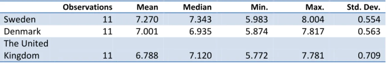
The descriptive statistics explain the nature of the data used in the analysis. For each variable, the mean, median, minimum, maximum and standard deviation values are presented to give an overview.
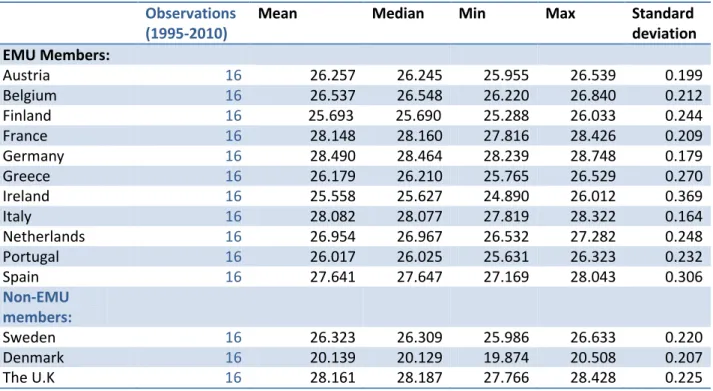
In Table A 3.1 in Appendix 3, we present descriptive statistics for the GDP of all sample countries. All values are derived from the logged values of the real GDP. As it can be seen in the data, Germany has the highest average GDP, followed by the United Kingdom and France. All of the sample countries reach the maximum GDP in year 2010 and there are no significant declines in the GDP data. As of 2010, Germany still ranks the highest values for GDP, followed by the United Kingdom, France and Italy. However, as these values are real GDP, they do not reflect economic growth or GDP per capita. One should acknowledge that these values simply present the size of the economies of the sample countries despite their populations.
All of the non-EMU sample countries have relatively large economies except Denmark. Using the standard deviation data, we can calculate the coefficient of variation.12 In our case all coefficients fall under 1 % area. This signifies that our GDP data is distributed within a considerably normal range.
Table 5.3 presents the distances between the capitals of trade pairs. Distance is a time invariant variable in the model. We calculate the distance from the 3 non-EMU members to 11 EMU members. It shows that Sweden is, in average, furthest away from its trading partners; therefore we expect to observe its distance coefficient to be larger than Denmark and the United Kingdom in the model analysis. The United Kingdom is closest to its trading partners as it has the smallest value of the minimum distance. The standard deviation seems a bit higher than the recommended level. This signifies that our distance data is more dispersed than the GDP data. Due to the nature of the data, it is a natural result. Even though their boarders are close to each other, some countries are spread far apart, for example Sweden and Portugal or Sweden and Greece which these provide big outliers leading to higher values of standard deviation.
Table 5.3 Descriptive Statistics for Distance
We observe a total of 11 trading partners for Sweden. The total trade values between Sweden and all of its trading partners are considered as our dependent variable. For each country we have 16 observations since we investigate the period from 1995 to 2010. In total there are 176 observations. Germany is Sweden’s main trade partner. Sweden imports more than it exports to Germany. The connection between GDP and total trade value is already observable in Table A 3.3 in Appendix 3. Germany with the highest GDP, exports more than smaller sized economies. We can observe higher frequencies of fluctuations in trade data than in GDP data. Sweden trades the least with Greece, which might reflect the long distance between them and the difficulties of transportation. A similar pattern is shown for the countries that are physically far away
12 The coefficient of variation can be calculated by dividing the standard deviation by the mean. If it is
less than 5%, the sources are known to be in the reliable range of distribution.
Observations Mean Median Min. Max. Std. Dev.
Sweden 11 7.270 7.343 5.983 8.004 0.554
Denmark 11 7.001 6.935 5.874 7.817 0.563
The United
from each other. According to the recommended level, the standard deviation shows a relatively good fit as there are no significant outliers.
Again, a similar pattern is followed in Table A 3.4 in Appendix 3, for Denmark. Germany has the highest mean among the trading partners of Denmark. The large trade value between Germany and the Scandinavian countries can be due to the result of history as well as the language similarities as they all belong to the Germanic language area (Johansson, 1993). Greece, Portugal and Austria have the lowest trade amount. Rose (2000) finds positive correlation between trade and common language area, however this outcome is contradicted in the case of the Danish-Austrian trade. Nevertheless, one must acknowledge the fact that these values are absolute values of total trade and that they are not adjusted to their populations. Standard deviations show that there are no particular outlier values, as all of the values for the coefficient variation are below 2 %.
Table A3.5 in Appendix 3 presents the United Kingdom’s total trade value. It shows the exact same ranking in total trade value as previously mentioned; hence Germany has the highest mean value. Greece, Portugal and Austria have the lowest values. This displays the economic sizes matter to a great extent. Ireland is actively engaged in trade with the United Kingdom as they are physically close to each other. We can see that Ireland has always been a stable trading partner to the United Kingdom as its trade value did not fall under a certain level over the whole sample period. Furthermore Belgium has high mean, median and minimum values showing that it has largely been a stable trading partner of the United Kingdom, a reason of which may be historical aspects. Again, the standard deviation remains normal.
6. Empirical Analysis
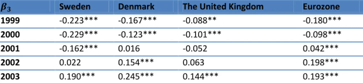
In this section, we present our main findings of the regression and analyze them more in-dept. We study whether there has been any visible euro effect after the members have entered the third stage of EMU and in addition its influence on the three non-EMU members. Furthermore, we observe if there has been any delayed effect of the euro on trade by lagging the euro dummy variable.
6.1
The Euro Effect on Trade
We analyze a panel of trade value using the random effects model, for the EMU countries and for three non-EMU countries over the period 1995 to 2010. The reason we have chosen to use the random effects model instead of the fixed effects model is because the fixed effects model cannot administrate time invariant variables such as distance and the EC dummy due to perfect multicollinearity. The same disadvantage of the fixed effects model has been recognized by previous studies as well (Penh, 2008). We include 176 observations for Sweden, Denmark and the United Kingdom. The observations are bilateral trade values between the above mentioned countries and the 11 EMU members over a 16 year period. Using the same method, we run a separate regression for the Eurozone countries with 1760 observations13.
Before we move on to the interpretation of the coefficient estimates, we need to elaborate further on the implications of the constant coefficients. As we have briefly mentioned in the theoretical framework, these constant values are time invariant and reflect unique trade relations between the interacting countries. These intercepts represent how stable the trade relation is between the two nations, considering the overall circumstances such as historical background, political system and language similarities. The majority of the intercept values presented on Table 6.1 are significant and negative. The negative constant can be interpreted as ‘stable trade’ between the trading partners. We refer the term ‘stable’ as a situation where there is a relatively less fluctuation in the case of GDP ups and downs in any one of the partner countries. We use a log-log model, thus the actual values of these negative constants are in fact, between 0 and 1 as it has been mentioned in Equation 1. Referring to the simple standard gravity model, we know that the larger the constant, the greater influence GDP will have on trade. By using the same logic, positive values indicate how ‘unstable’ the trades are between these country pairs, as they are greatly influenced by their economic performances. In our case, all values of the constants are negative which signifies comparatively small fluctuations in trade resulted by GDP changes.
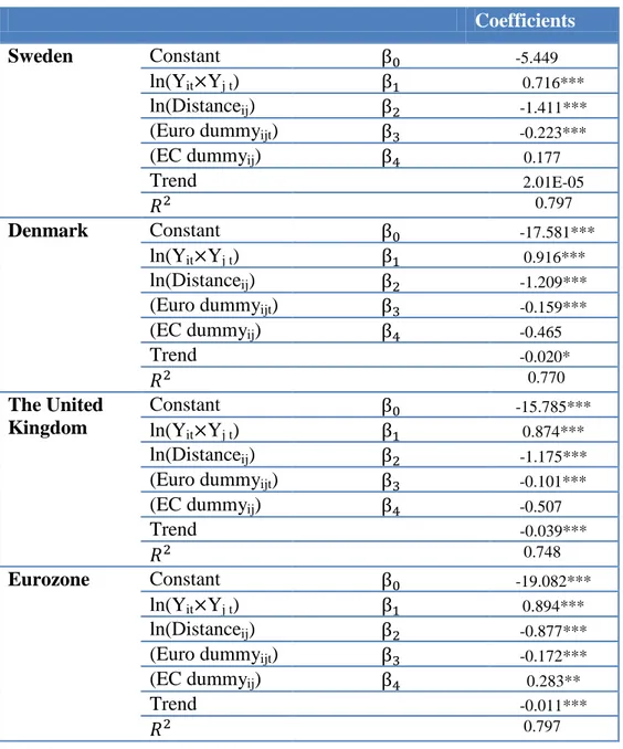
For the case of Sweden, is 0.716 and significant at a 1 % level, meaning that a 1% increase in will initiate 0.716 % increase in the total trade value between Sweden and the Eurozone countries. The distance variable is negatively related to the total trade value. The coefficient of distance is negative by 1.412. This result was expected as we know that longer the distance, extra costs are incurred resulting in smaller volume of trade between trading partners.
13 We run regressions of panel data for 11 countries, each of them with 10 trading partners over 16 year
periods which leads us to 1760 observations. We have utilized all the observations that we have access to, so the length of the time series are not subjectively chosen.
However, the negative figure shown on the coefficient of the euro dummy is rather surprising as this signifies that the implementation of the euro has had a negative impact on Swedish trade. As we will discuss more about this in the conclusion, this cannot be viewed as an absolute disadvantage of adopting the euro. The negative influence over the trade value can largely reflect ‘coincidental’ recessions in the European market after the implementation of the euro currency. In consequence, this could have tainted our estimates in certain ways. Another most probable reason is the possibility of a delayed effect (which is observable in the upcoming section of analysis). In many cases, policy adjustments take time until it produces any visible effect as there has to be a period of adaptation. This sequential effect on trade may also be expected for the euro implementation and is studied more in dept in Section 6.4.
Table 6.1 Panel EGLS (REM) output from EViews14.
14 *** significance at 1 % level
** significance at 5 % level * significance at 10 % level No star: insignificant
15 176 observations for three non-EMU members, Sweden, Denmark and the United Kingdom. 16
1760 observations for the Eurozone countries.
Coefficients
Sweden15 Constant -5.460**
ln(Yit Yj t) 0.716***
ln(Distanceij) -1.412***
(Euro dummyijt) -0.223***
(EC dummyij) 0.175
0.797
Denmark Constant -7.811***
ln(Yit Yj t) 0.718***
ln(Distanceij) -1.150***
(Euro dummyijt) -0.167***
(EC dummyij) -0.145 0.767 The United Kingdom Constant 3.943 ln(Yit Yj t) 0.476*** ln(Distanceij) -0.956***
(Euro dummyijt) -0.088 **
(EC dummyij) 0.243
0.722
Eurozone16 Constant -13.977***
ln(Yit Yj t) 0.802***
ln(Distanceij) -0.918***
(Euro dummyijt) -0.180***
(EC dummyij) 0.383***
Furthermore, the negative euro effect which implies the negative influence of the implementation on trade values can be resulted from Sweden being a non-member of the EMU however this seems unlikely for the two reasons. First, as it can be observed in Table 6.1, all of the other countries including the Eurozone countries seem to have negative figure on coefficients for the euro dummy as well, implying they are also influenced somewhat unfavorably by the implementation of the euro whether they are EMU or non-EMU members.
Other than the euro dummy, the EC dummy is presented. The EC dummy is included for two reasons. First, it is to see whether a country’s earlier entry to a free trade agreement such as the European Economic Community will increase its trade. Second, we investigate whether being engaged in trade with a founding member of the European Economic Community, which is an earlier form of a free trade agreement between the European countries, is beneficial to its trading partners. In this case, we see that there is a positive relationship between the trade value and being engaged in trade with the founding members of the European Economic Community. The estimates for the EC dummy are only significant within the Eurozone however; the estimates show positive patterns for both EMU and non-EMU members. For the case of Sweden, the largest trade partners are Germany and the Netherlands, both founding members of the European Economic Community. Therefore, the high estimates on the EC dummy coefficient is a natural result and it is not solely because they are founding members but also due to the relatively large size of these countries’ economies. The causality between the free trade agreement and size of their trade value is still ambiguous. Despite the ambiguity in this matter, it is indicated from this coefficient, that being a trade partner with one of the EC founding members is beneficial for Swedish trade. The negative constant value of indicates that the Swedish trade is fairly stable to the changes in GDP of home and foreign countries.
Denmark shows similar patterns to Sweden in all its outputs. All values are significant except the EC dummy. The constant is again a negative value which is -7.811. Denmark is not so sensitive to GDP changes therefore economic recession will have comparatively less impact on the Danish trade than the two other non-members. Denmark’s being the overall economic activity (Yjt Yit), is again positively
correlated to trade. For a 1% change in GDP, the Danish trade will increase by 0.718%. Again, the distance is negatively related (-1.150) meaning that the increased distance will hinder trade between the partners. The euro dummy is -0.167. The euro dummy coefficient shows that the Danish trade with the EMU members has comparatively decreased less than the United Kingdom and Swedish trade since the monetary unification. It can be due to many reasons. The Danish economy might not have been significantly influenced by economic downturns shown by the constant estimates and thus have stronger ties with its trading partners. In addition, it is possible that the Danish economy is more responsive to any positive impact initiated by the euro creation and its trade starts to recover already in 1999 however, not large enough yet to show a positive coefficient. In the case of Denmark, the EC dummy is insignificant showing no definite evidence of positive aspects of being a member of the European trade agreements. It is contradicting the past result of positive impact shown on the Eurozone trade however, there is little evidence to explain this contradiction. It can only be assumed that
Denmark, being geographically close to the European ‘mainland’, had already established a stable position in the European trade market. Thus, the European trade agreements had no particular impact on its trade.
For the case of the United Kingdom, three of the coefficients; GDP, distance and the Euro dummy, are significant. GDP is positively related to the total trade value where a 1% change in GDP will increase the trade value by 0.476%. Distance shows a negative value of -1.030. It implies that an increase in distance will negatively influence trade between the partners. The euro dummy however, reflects an unfavorable influence on trade again. It is estimated to be -0.163. The similar reflection can be made above on the causes of the negative euro effect in the case of the United Kingdom as well.
Lastly, the Eurozone has all its coefficients significant at a 1% level. The constant is negative meaning that the trade value is relatively stable to fluctuations in GDP. For a 1% change in the overall economic activity, trade will increase by 0.802%. Again, distance is negatively related as it shows a coefficient of -0.190. The euro dummy shows a negative impact on trade among the member countries with a coefficient of -0.180. This is an interesting result as we expected the euro dummy to capture favorable outcomes in the trade values for the countries that are in the common currency area. However as previously discussed, there could have been a delayed effect of the euro which is not visible yet.
Our outcomes can be summarized into five main findings. First, the euro dummy coefficients for all our sample countries, both EMU and non-EMU signify a downward trend in trade values since the year of the monetary unification. There are many possible reasons for these outcomes. The United Kingdom might have been largely influenced by the European sovereign debt crisis as its economy is largely dependent on the Eurozone countries. The same reason applies for the Swedish trade and the trade among the EMU members, as they have experienced significant decreases in economic performances during the past few years, this could have contaminated our investigation on the sole impact of the common currency area. Furthermore, we cannot overlook the delayed effect of the euro currency as the currency unification requiring time to settle in before its effect is noticeable.
Second, the euro dummy coefficients for Denmark and the United Kingdom show that their trade values have comparatively decreased less to the Eurozone since the euro creation. The cost of changeover probably has played role in downsizing the positive euro effect on EMU members since they are still in the adjusting phase of the new monetary measures. This assumption is supported by our theoretical parts where we discussed the costs of establishing an optimum currency area. Another possible reason for the less negative influence on the Danish and United Kingdom’s trade can simply be that fact that these two are more responsive towards the benefits of having an optimum currency area but at the same time, not bearing the costs of establishing it.
However, these cannot offer the full spectrum of the reasons behind the decreasing trend in trade values since the euro implementation. We recognize that the limitations of our empirical model might have tainted the results in some ways. The negative coefficient on the euro dummy coincides with Rose’s (2000) statement, where he claims that it is possible for a simple gravity model to have a null or negative coefficient due omitted
variables. Moreover, the short sample period might have caused the negative euro effect as we only include the years containing particularly low GDP growth17 after the euro creation. Especially in 1995, the data shows high figures in the exports for the many sample countries, compared to 2009 when the value decreases significantly. Furthermore, there can be lagged effects of the euro on trade which cannot be shown in the year 1999. We will develop this idea further in sub-section 6.4.
Third, we have verified that the assumption on the positive relationship between the overall economic activity ( ) and trade is true. Therefore, achieving greater GDP will increase trade values as well.
Fourth, distance is negatively related to trade value as it has been supported by many previous studies. It implies that an increase in distance will lead to decreased trade between the partners.
Lastly, the EC dummy is important for EMU nations, however, it appears not to be significant for non-EMU countries. Therefore, we cannot make a general assumption that EC initiates more trade between the all members of the European Union. It means that for the current members of EMU, it is more beneficial to be a founding member of the European Economic Community or to engage in trade with a founding member, whereas it does not play a big role in trade values for non-EMU members.
In conclusion, the euro effect on trade value for the three non-EMU members seems to decrease the trade values among EMU and non-EMU-members for various reasons. However, it is yet too early to conclude that the implementation of the euro has decreased trade for both EMU and non-EMU members. This leads us to Section 6.4 where we study the delayed effect of the euro implementation.
6.2
Diagnostic Tests
In order to evaluate the robustness of our empirical findings, we have conducted several tests for the residuals of our samples analysis.
The normality test for the sample countries shows non-normally distributed residuals for all countries except one, namely Denmark. Referring to Table 6.2, for Denmark, the skewness is -0.101≈0.00, the Kurtosis is valued at 2.742≈3.00, and the Jarque-Bera test statistic is 0.829. In addition, the probability of obtaining such a statistic under assumptions of normality is 66.1%. Thus, one can state that the null hypothesis of the residuals being normally distributed cannot be rejected in the case of Denmark.
For the case of Sweden, the null hypothesis of normally distributed residuals is rejected. As it is shown in Table A5.1 in appendix 5, the residuals are rather asymmetric. The normality test for Sweden presents a value of the skewness close to zero, referring to Table 6.2. The given kurtosis is approximately 2, while the JB statistic is 4.261 with a 11.9% a probability of obtaining such a statistic under assumptions of normality. Thus, we conclude that the residuals for Sweden are non-normally distributed.
17
This is similar to the case of the United Kingdom. The obtained kurtosis, with a value of 1.799, is below the value assumed for normally distributed residuals. There are extreme outliers measuring a rather high frequency in comparison to the other residuals as referred to Figure A5.3 in appendix 5, one might state that the distribution is rather turbulent. Thus, the kurtosis has been tainted by the extreme outliers. The skewness has a value of 0.184 while the JB statistic is measured at a value of 11.577 with a 0.3% probability of obtaining such a value under normally distributed conditions. Thus, one may conclude the null hypothesis of normally distributed residuals for the United Kingdom to be rejected.
Regarding the Eurozone, we see that the histogram for the Eurozone is non-normally distributed referring to Figure A5.4 in Appendix 5. There are some outliers contributing to the asymmetric shape of the histogram giving a value for the skewness of -1.294. The kurtosis has an extreme value of 9.342 while the JB statistic is extremely high with a value of 3440.770 with a probability of obtaining the value under normal assumptions being 0%. Thus we conclude that the null hypothesis of normally distributed residuals for the Eurozone is rejected.
Table 6.2 Normality Tests
Residual Normality Testing
Country Skewness Kurtosis Jarque-Bera Probability
Sweden -0.101 2.265 4.261 0.119
Denmark -0.108 2.742 0.829 0.661
UK 0.184 1.799 11.577 0.003
Eurozone -1.294 9.342 3440.770 0.000
Table 6.3 Panel Autocorrelation tests
Residual Autocorrelation Testing (Panel Breusch Godfrey Test)
Country Test Statistic
Sweden 6.030
Denmark 5.875
UK 6.281
Eurozone 6.314
Regarding the tests for autocorrelation among the residuals, Breusch-Godfrey tests have been conducted with the test statistic represented in Table 6.3. We can see that the null hypothesis of no autocorrelation among the residuals is not rejected at a 1% level for any of the sample countries. Regarding Sweden, the test statistic has a value of 6.030 being less than 13.28 which is the at a 1% level18. The similar observation is made on Denmark with a test statistic of 5.875 and the United Kingdom showing a test statistic of 6.281. The Eurozone shows a similar result with a test statistic of 6.314. Thus, as previously stated we cannot reject the null hypothesis of no autocorrelation among the
18
residuals at a 1% level regarding all our sample countries. We can conclude that the residuals of the sample countries do not have autocorrelation problems.
6.3
The Euro Effect on Trade with Time Trend Variable
Addition to the findings above with the modified version of the gravity model, we have constructed a second set of analysis with a time trend variable, . This is conducted in order to investigate the robustness of our previous analysis which does not include the time trend variable. The addition of the time trend variable in the new model allows us to adjust for non-stationary data and to remove deterministic trend in the regression, however it is important to denote that stochastic trends are not considered in this study.
( ) ( ) ( ) + +
t is a time index
Equation 6. Empirical gravity model with time trend
Bun and Klaassen (2007) made an extensive study on the use of the time trend variable in discussing the euro effect. They avoided a trend misspecification when examining the euro dummy by adding a specific time trend for each trading partner, thus amending for upward trends in trade flows over the years. The ‘country-pair-trending variables’ capture the upward trend initiated by omitted variables, therefore the deterministic trend is not reflected on the euro dummy coefficient. In our model, we do not use a country-pair specific trend variable for each trading country-pair however; we assume that the trend is common between home countries to all its trading partners. This might seem to be a strong assumption, nevertheless, it is evident that trade relations between the European countries do not vary to a great extent as their business cycles are converged due to extensive market integration in the European Union. Fluctuations tend to have similar magnitudes among the members as it has been shown in Figure A2.1 and A2.2 in Appendix 2. Despite the assumption made, we are aware of the limitations of using a unified time trend variable for all independent variables as it is possible that an upward trend caused by the implementation of the euro can be amended by the time trend variable. However, this is left for the further studies.
For comparative purposes, the new outcomes are presented in the same format as the outcomes without the time trend, therefore we can evaluate whether the former estimates are inflated due to trend misspecification.
Table 6.4 shows that the introduction of the trend variable is significant for all countries except for Sweden. However, in spite of the trend variable being insignificant for Sweden, the coefficients of the remaining variables show small changes when adopting the time trend variable. After introducing the time trend, becomes insignificant. On the other hand, the EC dummy remains the same and it is still insignificant. However, the remaining variables do not present large changes in its coefficients in comparison to Table 6.1.