Aggregation in organic light emitting diodes

A thesis submitted to the Faculty and Board of Trustees of the Colorado School of Mines in partial fulfillment of the requirements for the degree of Master of Science (Applied Physics).

Golden, Colorado Date________________________ Signed: _____________________________ Abigail Meyer Signed: _____________________________ Dr. Jeramy Zimmerman Thesis Advisor Golden, Colorado Date ________________________ Signed: ____________________________ Dr. Jeff Squier Professor and Head Department of Physics

ABSTRACT

Organic light emitting diode (OLED) technology has great potential for becoming a solid state lighting source. However, there are inefficiencies in OLED devices that need to be under-stood. Since these inefficiencies occur on a nanometer scale there is a need for structural data on this length scale in three dimensions which has been unattainable until now. Local Electron Atom Probe (LEAP), a specific implementation of Atom Probe Tomography (APT), is used in this work to acquire morphology data in three dimensions on a nanometer scale with much better chemical resolution than is previously seen. Before analyzing LEAP data, simulations were used to investigate how detector efficiency, sample size and cluster size affect data analysis which is done using radial distribution functions (RDFs). Data is reconstructed using the LEAP software which provides mass and position data. Two samples were then analyzed, 3% DCM2 in C60 and 2% DCM2 in Alq3. Analysis of both samples indicated little to no clustering was present in this system.

TABLE OF CONTENTS ABSTRACT…..……….…iii LIST OF FIGURES………....v LIST OF EQUATIONS……….…vi ACKNOWLEDGMENTS………....vii CHAPTER 1 INTRODUCTION………..1

1.1 Introduction and Significance……….1

1.2 Principles of OLED Operation………....4

CHAPTER 2 SCOPE AND METHODOLOGY……….11

2.1 Survey of Literature………...11

2.2 Scope of Research……….……….13

2.3 Method……….………..15

CHAPTER 3 DATA COLLECTION AND ANALYSIS………..17

3.1 Simulated Data………..……….17

3.2 Experimental Data……….………24

3.3 Data Analysis……….………26

3.4 Investigation of Reconstructions……….………...31

CHAPTER 4 CONCLUSIONS AND FUTURE WORK………35

REFERENCES CITED……….……….37

LIST OF FIGURES

FIGURE 1.1 Basic organic light emitting diode structure. Modeled off of reference [10]……..5

FIGURE 1.2 Energy transport mechanisms. Adapted from reference [18]………..7

FIGURE 2.1 Molecules used to create preliminary OLED systems………...14

FIGURE 2.2 Example radial distribution function graph……….………..16

FIGURE 3.1 Body centered cubic and face centered cubic radial distribution function………17

FIGURE 3.2 Random close packed structure radial distribution function plot………..19

FIGURE 3.3 Radial distribution function plot of dimers from various parent sample size……21

FIGURE 3.4 Detector efficiency comparison of dimers……….22

FIGURE 3.5 Comparison of various cluster sizes………..23

FIGURE 3.6 Mass spectrum of DCM2 in C60………..24

FIGURE 3.7 Mass spectrum of DCM2 in Alq3……….………..25

FIGURE 3.8 Radial distribution function of DCM2 in C60………..………...27

FIGURE 3.9 Radial distribution function of DCM2 in Alq3……….………..29

FIGURE 3.10 Concentration map of different reconstructions………32

LIST OF EQUATIONS

EQUATION 1.1 Rate equation of energy transfer in Forster radiation………..7

EQUATION 1.2 Critical distance when Forster radiation is 50% efficient………8

EQUATION 1.3 Spectral overlap………...8

EQUATION 1.4 Efficiency of Forster radiation……….8

EQUATION 1.5 Rate equation for dexter radiation………....8

EQUATION 1.6 Quantum efficiency of emission due to triplet triplet annihilation………..9

ACKNOWLEDGMENTS

I would like to thank several people for their contributions to this project. The first person I would like to thank is my thesis advisor Dr. Jeramy Zimmerman whom not only came up with the initial idea for the project but whom also provided invaluable guidance throughout the project. I would also like to acknowledge Andrew Proudian. He took the atom probe data as well as created the function space I worked with in R. I would also like to acknowledge Mathew Jaskot, the other member of our research group. I would also like to acknowledge the members of my thesis committee, Dr Thomas Furtak and Dr Alan Sellinger, for their time and input. Fi-nally, I would like to acknowledge the Colorado School of Mines for use of lab space and equip-ment.

CHAPTER 1 INTRODUCTION

In recent years, organic light emitting diode (OLED) technology has undergone a re-newed appearance in the scientific community. OLEDs have made remarkable strides in the dis-play field as OLED disdis-plays draw less power than liquid crystal disdis-play (LCD) technology [1]. OLED displays can be made thinner as they contain no backlight, which an LCD display must encase [1]. In addition, an OLED display needs fewer components. For example, an OLED dis-play does not require a polarizer.

1.1 Introduction and Significance

OLED technology could also make great strides in the field of lighting. One reason OLED technology would be advantageous is that it can be made incredibly thin and flexible. OLED light sources are intrinsically large area which makes them ideal for lighting. As such, OLED technology does not need a diffuser which a light emitting diode (LED) must contain in order to produce useful light because LEDs are point sources. Also included in LED technology is a heat sink which an OLED does not need. One final advantage of OLEDs is that their color rendering index (CRI) value is very good. A CRI value indicates how well, on a scale from 0-100, a light produces the desired color. OLED lights can achieve CRI values of 90 and above while most LED lights can only achieve CRI values of 90 or less [2].

There are still roadblocks to transitioning from traditional lighting methods to OLED technology, such as OLEDs tend to degrade quickly. At present the most troublesome OLED color is blue with an average lifetime of around 20,000 hours [3]. In order for OLED lighting to

be commercially viable they must have a lifetime on the order of 30,000 to 60,000 hours [4]. At the present time this lifetime goal is attainable for colors such as red and green but is not yet achievable for blue. Another such roadblock is that OLED technology is not yet sufficiently effi-cient. Fluorescent lighting efficiencies are at 50-70 lm/W [5] and LED lighting efficiencies are at 50-100 lm/W [5]. Commercially available OLED displays have efficiencies around 60 lm/W which is comparable but still on the lower end of these ranges [6] and small improvements to de-vices could lead to large impacts on efficiency.

There are three main factors that lower phosphorescent OLED quantum efficiency: con-centration quenching, triplet-triplet annihilation (TTA) and triplet-polaron annihilation (TPA). These mechanisms will be detailed later in section 1.2. In summary, concentration quenching is a lowering of emission quantum efficiency as concentration of the guest emitter in the host material is increased. Triplettriplet annihilation is when two triplets come close enough to one an other to interact. The two triplet states will combine to create a ground state singlet and an ex -cited singlet. Triplet-polaron annihilation occurs when an ex-cited triplet interacts with a charged molecule, eg a polaron, to lose energy [7].

Another factor to consider is aggregation, which is when guest molecules clump together, which lowers brightness. Ideally guest molecules would be randomly distributed in the material. When guest molecules are closer than is ideal there are more possibilities for excited states to re-lax via dark pathways, simply because they are closer together and can more easily interact. At present there is very little data which can show precise distribution of these factors as well as the

In order to discover the extent to which these factors affect efficiency and brightness of an OLED there is a need for investigation of OLED morphology at a smaller length scale. Cur-rently the only small scale data on aggregation phenomena in an OLED is recorded at a nanome-ter scale in two dimensions via tunneling electron microscopy [8]. While this picture gives some insight into the efficiency issues in OLED materials it does not describe the whole physics. In or-der to fully unor-derstand loss mechanisms and structure, data needs to be in three dimensions.

In this work we introduce the use of Local Electrode Atom Probe (LEAP) tomography, a specific implementation of atom probe tomography (APT), to elucidate the physics of aggrega-tion in OLEDs. In doing so, we will be able to gain informaaggrega-tion at a nanometer scale in three di-mensions. Once we obtain data from this system we will analyze the data using radial distribu-tion funcdistribu-tions to determine how randomly the molecules are dispersed in the sample. From there we will make further conclusions about the degree of aggregation. Once this is complete we will compare different OLED systems in order to discover how to minimize aggregation therefore in-creasing efficiency of OLED devices.

This project has several important impacts in the field of OLEDs. Firstly, this project will move into uncharted waters in terms of investigation in OLEDs. No other studies, as far as we are aware, have used APT technology to analyze OLEDs. This will be an important step towards understanding aggregation and the underlying physics which govern OLED behavior.

In addition, this project has obvious scientific merit in that it will increase our knowledge of structural properties of an OLED. Being able to study OLED materials at the nanometer scale will allow for a deeper understanding of aggregation as well as photophysical properties of

OLEDs. This knowledge will lead to better OLED models and better numerical reconstructions of processes happening within an OLED, such as how excitons are diffusing and recombining.

Finally, this project has economic benefit. If aggregation can be decreased in OLED de-vices, less of the expensive emissive materials would be used in order to produce these devices. If the devices are less expensive to produce they would make more headway in replacing current lighting technology. In addition, if aggregation and concentration quenching are decreased, OLED devices would be more efficient. If the efficiency doubles within an OLED the same amount of light can be produced with half the area. This would reduce cost of all materials used to create an OLED, making them much more cost effective. This added efficiency would be an-other push to replace current lighting technology with OLEDs.

1.2 Principles of OLED Operation

An OLED is a semiconductor device, which produces light. OLED devices are typically made out of many different materials which each have a specific purpose. A schematic diagram of a typical OLED is shown in figure 1.1 (see page 5).

OLED devices are commonly created in a layered structure. The anode, typically indium tin oxide (ITO), is deposited onto a glass or plastic substrate. A hole transport layer is then de-posited to aid in the movement of holes while blocking electrons from leaving the emission layer. The emission layer is the most important, as it is where excitons recombine to emit photons. Of-ten, the emission layer is doped with a fluorescent or phosphorescent dye in order to aid in pho-ton emission from the device. Electrons are injected by the cathode, usually a metal, and through

Polarons, i.e. holes and electrons, meet in the emission layer and combine to create exci-tons. An exciton is an electron-hole pair, which is bound by a Coulomb force. Statistically, 25% of excitons are formed in a singlet state, where the exciton has a magnetic and spin quantum number of zero [9]. This singlet state has one spin up and one spin down vector out of phase with one another [10] and is optically active [10] as the transition is allowed via quantum mechanics. However, 75% of excitons are created in the triplet state. This is a degenerate state where the spin quantum number is 1 and the magnetic quantum number is -1,0, or 1 [9]. The spin quantum number makes triplet states very different from singlet states. In the case of these triplet states, when the magnetic quantum number is 0 there is one spin up and one spin down vector but they process in phase which gives a spin vector perpendicular to the axis about which the spin vectors rotate [9]. When the magnetic quantum number is 1 or -1 both spin vectors are either up or down

Figure 1.1: Basic organic light emitting diode structure. Modeled off of a picture in reference [10].

respectively [9]. Since the spin vectors are parallel they are no longer paired as is the case in a singlet state. This means that these triplet states are optically inactive because the transition is forbidden. The transition is forbidden by the Pauli exclusion principle, as electrons of the same spin and magnetic quantum number cannot occupy the same orbital at the same time. In this way the transition is forbidden because triplet states consist of two electrons with parallel spins, so they may not relax into the same state.

As excitons are excited states, they will eventually relax. There are several different forms of recombination. In figure 1.2 (see page 7), there is a schematic of both radiationless and radiative recombination processes. Only two of these many pathways, fluorescence and phospho-rescence, will produce light. All others are radiationless. One radiationless process is intersystem crossing which is energy transfer between singlet and triplet states. Another radiationless process is internal conversion which occurs when an excited singlet state transfers energy to a vibrational singlet state. A third radiationless process is vibrational relaxation which is the creation of a phonon within a molecule. This can occur via defects in an imperfect film. Finally, Förster radia -tion can occur between the triplet state of one molecule and either a vibra-tional singlet state or excited triplet state of another molecule. All of these processes make for complex radiation path -ways in an OLED, especially since an OLED is amorphous. The more radiationless path-ways we can block, for example minimizing defects, the better the efficiency of the OLED.

Excitons can also diffuse within the emissive layer via energy transfer. The first type of energy transfer is Förster radiation (also known as Förster resonant energy transfer or FRET)

which is a radiationless transfer mechanism [9]. Förster radiation occurs via a dipole-dipole in-teraction. An excited electron will create an oscillating dipole causing an electric field [9].

This electric field can induce a dipole in neighboring molecules. If this occurs, and the two dipoles are in phase with one another, these two dipoles can couple [9]. This coupling interaction can cause the original excited electron to relax and an electron in the induced dipole to be ex -cited, thereby transferring energy [9]. The rate equation of energy transfer in Förster radiation is given by [11]

In this equation, τD stands for the excited state lifetime of a donor molecule in the absence of an acceptor molecule analogous to lifetime of a free carrier in a diode, Ro stands for the critical dis-tance which is the disdis-tance between a donor and acceptor molecule when Förster is at 50%

effi-Figure 1.2: Depiction of energy transport. Molecule A shows the energy transport within one molecule including fluorescence, phosphorescence, intersystem crossing (ISC), internal conversion (IC), and vibrational relaxation (VR). T is used to denote a triplet energy while S

denotes a singlet energy. Molecule B demonstrates Förster radiation between the two neighboring molecules. Adapted from reference [18].

ciency, and R is the distance between the donor and acceptor molecules in question [11]. Ro in angstroms is defined as [12]

In the above equation the constant accounts for units, κ is the orientation factor, Φ is the quantum yield of the donor's fluorescence, n is the refractive index of any intervening medium and J is the spectral overlap of the donor's fluorescence spectrum and the acceptors absorption spectrum. J is defined as [12]

In this case F is a normalized donor fluorescence spectrum, ε is the maximum molar extinction coefficient of the acceptor, and λ is wavelength. The efficiency equation of this process is de-fined as

The second type of energy transfer is Dexter radiation, where an excited electron and hole tunnel from one molecule to another [9]. The rate equation for dexter radiation is given by [13]

(1.5) (1.4) (1.3) (1.2)

In this equation K is a constant determined experimentally, J is the normalized spectral overlap integral, RDA is the distance between a donor and acceptor molecule and L is a sum of Van der Waals radii [13]_.

We plan to elucidate three main factors that effect OLED quantum efficiency, as previ-ously mentioned. Firstly, concentration quenching occurs through multiple Förster radiation pro-cesses which occur sequentially [14]. As concentration of the guest molecule increases, the size of guest aggregates also increases [15]_. In this way there are more non-radiative pathways simply because the guest molecules are closer together in space. Being closer in space means there are more chances for excited states to interact and recombine via a dark pathway as there are more dark than emissive pathways. Secondly, TTA occurs when two triplets get close enough that they are able to interact. In TTA two excited triplets combine to form an excited singlet and a ground state singlet [16]_. In this case, since TTA requires two triplet states, the rate of TTA should in-crease with the square of the concentration of excited triplet states [16]. If TTA is the main loss mechanism, the quantum efficiency of emission is approximately [16]:

Where η is the efficiency which is being solved for, ηo is the efficiency in the absence of TTA, JT is defined as [16]:

(1.7) (1.6)

Additionally, q is the charge on an electron, d is the thickness of the exciton formation zone, kq is the triplet quenching parameter, τ is the phosphorescent recombination lifetime and J is the cur -rent density.

Finally, as previously stated, TPA occurs when a triplet state and a charged particle come close enough to interact, generating a charged particle and a ground state particle [7]. This process can only occur in materials where there is an excess of free charged particles in the mate-rial.

A prominent contribution to loss is emitter aggregation [17]-[18]. Aggregation increases TTA [19] because clusters take the same number of triplet states that would be present in a ran-dom dispersion of molecules and place them in a smaller volume. Putting these triplet states closer together will increase the probability of TTA, since TTA goes like the square of concentra-tion, and producing singlet states. In addiconcentra-tion, putting molecules closer together causes a red shift, or a reduction of energy, of the expected fluorescence. This occurs because fewer mole-cules are relaxing via fluorescence or phosphorescence and more are relaxing via dark pathways. When there is a region of lower energy, excitons will be concentrated in this region, further in-creasing TTA. Another reason aggregation is a problem is that as molecules group together it is more likely that excitons will recombine via dark pathways, as previously mentioned. This means that clusters actually inhibit photon production. As clusters get bigger they inhibit photon production more hence aggregation’s contribution to concentration quenching.

CHAPTER 2

SCOPE AND METHODOLOGY

There are several studies which discuss local order in OLED materials. They try to eluci-date the structural properties of OLED materials and they are a good starting point for this work, however they do not contain enough structural information to understand things like exciton dy-namics.

2.1 Survey of Literature on Aggregation in OLEDs

M. A. Baldo et al. studied thin film materials containing polar molecules and found that local order in amorphous thin films due to polarity caused a shift in the fluorescent spectrum [20]. This means that structural changes, even in an amorphous film, can cause shifts in an output spectrum. J. Gong et al. studied the effect of heating in a BT in TBPI OLED device and found that as temperature increased the device exhibited phase separation, aggregation and decreased photoluminescence [21]_. They then probed band gaps and found that neither materials' band gap had changed. They concluded that the decrease in efficiency must be due to a structural change but they did not have the resolution to prove it. A. R. G. Smith et al. studied Ir(ppy)3 in CBP and investigated the effect of thermal annealing [22]. They found that 6 wt% of Ir(ppy)3 had more phase separation that 12 wt%. They also discovered that annealing caused a layer adjacent to the emissive layer to mix. This mixing caused changes in device performance as well as morphol-ogy. Again, they noticed these morphology changes but did not have the resolution to probe them further. G. L. Ingram et al. reported recent increases in OLED efficiency as well as brightness as it pertains to use of OLEDs in solid state lighting technology [23]. They cite improved exciton

management as the reason for these increases and suggest that a greater understanding of exciton travel in OLEDs is needed in order to continue innovation.

Although many studies on concentration quenching in OLED devices exist, few contain

microstructural analysis. Y. Q. Zhang, et al. studies neat fac-tris (2-phenylpyridinato-N, C2

_’)

iridium (III) [Ir(ppy)3] emitting layer devices [24] and found that phosphorescent emission de-creased as Ir(ppy)3 thickness inde-creased. It was believed that this decrease in emission, or concen-tration quenching with respect to electroluminescence, was due to TTA. So, as Ir(ppy)3 concen-tration increases, there is a higher chance that triplet states will be close enough to one another to interact and annihilate. This interaction is at least partially responsible for decreased light emis -sion in the device. N. C. Giebink et al. investigated external quantum efficiency in four different OLED systems and discovered that decreases in efficiency were either due to quenching or loss of charge balance [25]_. They also suggest that OLEDs which maintain charge balance at a high current density may allow for decreased or even eliminated efficiency decreases. J. S. Price et al. analyzed OLED electroluminescence in order to quantify annihilation rates in fluorescent and phosphorescent OLEDs [26]. They derive an analysis of quenching which can be conducted solely on light-current-voltage measurement data.

Another important result found in the literature is a noted red shift in OLED devices as dopant concentration is increased. One study demonstrates this red shift in Alq3 devices doped with C540 [27]. This study noted that the fluorescent intensity of these devices initially increased with a doping concentration of 0.5%. As doping concentration increases beyond that the intensity

in Alq3 [28]. This study noticed a 36 nm red shift as the concentration of DCJMTB was varied from 0.5% to 3%. They also noted a marked change in emission color of the devices from orange to red as well as a decrease in luminance efficiency as seen in the previous study.

2.2 Scope of Research

Concentration quenching is a challenge that, if reduced or suppressed, would largely im-prove the performance of OLED devices. Aggregation in particular needs to be at the very least quantified. While clusters have been shown to exist in one system [19], this two dimensional im-age does not give much quantitative information about the clusters because one cannot see how many emitter molecules are present in each cluster. For example, on a quantitative molecular scale one could look at different materials and really understand what combination of guest and host materials aggregate less. Once this is determined one could make conclusions about what causes aggregation and work to counteract it.

This thesis will quantify aggregation in OLED devices at a molecular scale. Once data is collected using atom probe tomography (APT), a non-traditional technique for the analysis of OLEDs, to be discussed in the method section, we will analyze the data provided to discover how much aggregation occurs in guest-host systems. Once the system has been analyzed, we will draw conclusions about which device properties cause aggregation and how to reduce overall ag-gregation in OLED devices.

Detailed steps for this research are detailed as follows. We will analyze commercially available OLED systems such as [2-methyl-6-[2-(2,3,6,7-tetrahydro-1H,5H-benzo[ij]quinolizin-9-yl) ethenyl]-4H-pyran-4-ylidene] propane-dinitrile (DCM2) in

tris(8-hydroxyquinolinato)aluminium (Alq3). These systems will be analyzed using APT. A depiction of the molecules we plan to use can be seen in figure 2.1. First, APT data will be analyzed using ra-dial distribution functions for 2% DCM2 in Alq3 as well as 3% DCM2 in C60 for comparison. This data will be compared against statistical models of clustering which have been created. Models were first developed for cubic, face and body centered cubic lattices which will be ran-domly populated with 1% of a molecule. These models will be used to calibrate parameters in the functions used to analyze the data. Next a realistic simulation needed to be created for OLED films. Since OLEDs are amorphous films a random close packed structure was chosen. These structures are created in a fashion that is analogous to pouring marbles into a box. The first layer is placed in the box so that it covers the whole box area. Next, a second layer is deposited on top of that and shaken until all of the marbles settle. This is repeated for consecutive layers. The first few layers will appear crystalline but by the third or fourth layer marbles will be randomly ar-ranged. These random close packed structure models will be used to create dimers and various larger clusters. They will also be used to analyze detector efficiency effect and determine how large the sample size needs to be to give data with low noise.

2.3 Method

The guest-host systems will be created via vacuum thermal evaporation onto a tip which is a tungsten probe typically with a radius of 500 nm. We will analyze the systems using Local Electron Atom Probe (LEAP). The LEAP applies a bias to the probe shaped sample. The tip will then be heated using a pulsed laser which serves to evaporate ions off of the surface. These ions will be accelerated by an electric field to a 2-dimensional detector. The time which the ion takes to travel to the detector, or the time of flight (TOF), allows for a chargetomass ratio to be calcu -lated. The starting position of the ion is calculated using electric field data as well as the position where the ion hits the detector. A 3-dimensional image of the sample is generated by the LEAP software. LEAP has never before been applied to OLED systems. However, this system is known to give resolution at a much smaller scale, on the order of nanometers, as well as at a better chemical resolution than existing analysis techniques. This system has been used by others in my research group to give very accurate data at a small scale in organic photovoltaic systems. We therefore suggest that LEAP can also be similarly helpful in OLED systems.

LEAP provides position and mass data of each molecule detected, however the LEAP de-tector only detects a maximum of 58% of the molecules. This efficiency needs to be accounted for both when analyzing data and when creating the aforementioned simulations. We then will analyze this data using the radial distribution function (RDF). RDFs analyze data by choosing one molecule as a center. Spherical shells of incremental thickness are then drawn around a cen-ter molecule. The function then tracks how many neighboring molecules lie in each shell divided by the volume of the shell so that it goes to 1. This process is repeated using each atom as a

cen-ter but excluding any previous molecule which has already been used as a cencen-ter point. The RDF is described by g3(r) = K'3(r) / (4*pi*r^2) where K3(r) = (1/lambda) E(N(Phi,x,r) | x in Phi). In the previous equation lambda is defined as the intensity of the point process, Phi is the point process, N is the number of points in Phi other than the point itself x which fall within a radius r of x and E denotes an expectation value. For a perfectly random system we expect to see a peak after some initial radii below which no molecule can exist due to repulsive Pauli interactions. Af -ter this initial peak we would expect to see decreasing oscillations about one. In other words, we expect to see a Poisson distribution if the system is perfectly random. An example RDF can be seen in figure 2.2 below. If clustering exists we expect to see data which is skewed in some uni-form way from a Poisson distribution. This could mean that the initial peak is much higher than predicted as molecules are closer together than they would be in a random system. This RDF analysis will be carried out using a computer program, namely R.

CHAPTER 3

DATA COLLECTION AND ANALYSIS

Since LEAP has never before been used on OLED devices there is a need to develop sim-ulations which assist in understanding experimental data. These simsim-ulations were developed in R because of its ability to handle large data sets and preform statistics.

3.1 Simulated Data

The first task was to ensure that the built in radial distribution function in R, pcf3est, out-put plots that made sense. In order to do this a function space was created that allowed for simple cubic, body centered cubic (BCC) and face centered cubic (FCC) lattices to be easily output. Both BCC and FCC lattices were tested by creating a large sample and then randomly selecting one percent of the points out of this parent sample. The one percent sampling is desired because it is the doping concentration used in the emitter layer of many real devices. The output RDF was then plotted along with a scaled histogram of number of counts per distance in order to make sure that no peaks were missing. The resulting graph is shown in figure 3.1.

Figure 3.1: BCC and FCC lattice RDF. The broadened peaks are generated by the built in RDF and the discrete, black vertical lines are generated from the histogram.

As seen in figure 3.1 the built in RDF peak location matches well with the histogram peak location. This occurred after changing several parameters in the built in function. This is be-cause the built in function applies a smoothing kernel to the data. This smoothing kernel was broadening some of the peaks so much that they blended with neighboring peaks. The parameter delta, which is the half width of the smoothing kernel, was set to 0.05 units so that there was very minimal smoothing. The biascorrect parameter was also set to false which prevents compensa-tion for the value of the smoothing kernel near zero further avoiding manipulacompensa-tion of data in reference to the smoothing kernel. In addition, the maximum radius out to which the radial distribu -tion func-tion is calculated was set to 8 and the number of values of the radius which were tested for the RDF was set to 256 in order to improve run time of the code. Example code can be seen in appendix A.

Now that parameters for an accurate RDF generation of experimental data were under-stood, a reasonable simulation for OLEDs had to be chosen. OLED films are amorphous in most cases. As such, a random close packed structure (RCP) was chosen to simulate OLED films. The RCP structure is a reasonable approximation for the amorphous OLED materials. A RCP genera-tor program created by K. W. Desmond and E. R. Weeks was used to generate the building blocks for these structures [30]. This program had several input parameters contained in a config-uration file. The first was number of dimensions which was set to 3. Next was number of parti-cles which was most often set to 3000 as this created a high enough number of points for repro-ducibility of the simulation as well as giving a reasonable run time of the RCP generator. The

0.025 respectively. The size ratio and percent of small particles was set to 1 so that all particles were of the same diameter. The box size was set to be 10 units in each dimension and the bound-aries were all set to be periodic allowing for blocks to be stacked to create larger data sets with-out increasing the run time of the RCP generator. Finally, the tolerances were left as their default value and the seed number varied between trials. In using this program a variety of system pa-rameters were output. The most important was the final packing fraction. In all cases this packing fraction was within 1% of 63% which is expected for a close packed structure [31]. This means that the molecules were all packed as closely as they could be to one another allowing clusters to be created by simply comparing the sampled structure to the parent structure and selecting a de-sired number of nearest neighbor molecules.

The aforementioned building blocks were scaled to a normalized particle diameter of 1 unit. A representative RDF of this 3000 point building block can be seen in figure 3.2.

The first peak at r~1 corresponds to the nearest neighbor contribution. The second set of peaks at r~ 1.8 and 1.9 is due to the second nearest neighbor and so on. The dotted green line is at 1 which is the value all RDFs will asymptote to at large distances.

Once the building block was created 5 times with different seed numbers, or starting posi-tions of molecules, to test repeatability of the program the next step was to discover how large of a sample size was needed to reduce noise to acceptable levels. This was done by tessellating the building blocks to create various sizes of RCP arrays. This building block was 13.54 radial units on each side. Four parent samples were created ranging in size from a 3x3x3 cube of 3000 point building blocks to an 8x8x8 cube. Next 0.5% of the points in these large blocks were sampled and dimers, or clusters of two as can be seen in appendix A, were created because the first sam-ple will be doped with DCM2 which has a strong dipole moment and is expected to cluster strongly. This resulted in these dimer samples containing 1% of the parent block's number of points. Next 58% of the points in these 1% samples were randomly selected because the maxi-mum detector efficiency of LEAP is 58%. RDF plots for these four large block sizes can be seen in figure 3.3 (see page 21).

The largest parent sample size depicted in figure 3.3, the 8x8x8, has very low noise with a mean square error (MSE) of 0.012 which makes sense as this sample has the most data points and therefore error should be low. The MSE was taken between the data which fluctuates and the dotted line at 1 from r = 2.5 to 4 as we ideally expect this region to be 1. The 6x6x6 parent sam-ple also exhibited low enough noise, with an MSE of 0.019, that it would be viable to analyze.

The 3x3x3 and 4x4x4 sample sizes both exhibit larger oscillations about 1, with MSE = 0.053 and 0.049 respectively, and contain enough noise to cause issues in experimental analysis since ideally the MSE should be as low as possible. From the above graph it was decided that the 6x6x6 sample, which has the same volume as a 50 nm thick sample with radius 41 nm when we assume that our molecules are about 1 nm in diameter, would be the sample size we would aim for. This is because it is within the field of vision of the LEAP apparatus as well as being much thicker than initial data sets which proved to be to thin to see much of the dopant, which will be discussed further in the next section.

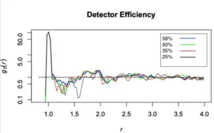
In the next simulations how the detector efficiency effects RDF plots is calculated. As the LEAP detector is maximally 58% efficient, it would be useful to know, for example, if an experi-mental sample was deposited with a specific number of dopant molecules how the RDF plot

changes as a function of detector efficiency. The 6x6x6 dimer data set was examined at a range of detector efficiencies between 58% and 25%. The RDF plots can be seen in figure 3.4.

Figure 3.4 demonstrates that the 58% and 50% detector efficiencies are relatively similar and give data with little noise, exhibiting MSE values of 0.019 and 0.028 respectively. Once we get to 35% efficiency the oscillations about 1 increase quite a bit compared to the previously mentioned cases, with a MSE value of 0.030. Finally, at 25% we lose most of the data after the nearest neighbor peak and the noise further out in r increases, with an MSE of 0.045. This loss of information makes it hard to examine cluster density and abolishes the second nearest neighbor information.

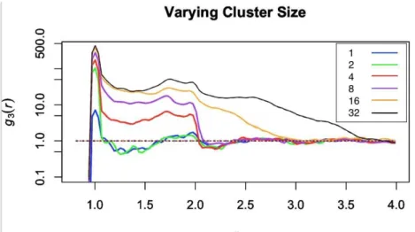
The final piece of information which needed to be gleaned from these simulations was how cluster size can be inferred through RDF analysis. In order to investigate this clusters were

cluster, along with an unclustered sample for comparison. Beginning with the 8x8x8 parent sam-ple since it had the lowest noise, samsam-ples were created such that each contained 1% of the parent number of molecules and then the data was sampled again at 58% detector efficiency which can be seen in figure 3.5.

As can be seen in figure 3.5 there are two notable changes as cluster size increases. The first notable change is that the nearest neighbor peak height increases. This increase happens each time cluster size increases but the effect appears diminished because the y axis is plotted on a logarithmic scale. The peak increase is also diminished because of a surface area effect. When the clusters are smaller, say 2 molecules, all of the molecules are surface molecules. However, when the cluster size increases, say to 32 molecules, very few of those molecules are surface molecules so they effect the peak size less. The second notable change is the smearing out of the decrease to one after the largest peak. This occurs because as the cluster size increases there is a

higher number of molecules right next to each molecule. For example, with dimers there will be one nearest neighbor, if it was not randomly selected out when detector efficiency was accounted for, and after that nearest neighbor there will be a larger distance between one dimer and the next so interactions die off quickly. However, with a cluster of 32 there could be up to 31 nearest neighbors before that interaction dies off, hence the slow decrease to one.

3.2 Experimental Data

The first sample for which data was acquired using LEAP was 3% DCM2 in C60. This sample provided a useful starting point in that DCM2 is very polar which should cause it to read-ily aggregate. C60 on the other hand is non-polar. The sample was created by thermally co-de-positing C60 and DCM2 such that the rate of deposition of C60 was much higher than that of DCM2. The sample was then kept in a glove box until it was transferred to the LEAP apparatus. Data was taken in the LEAP over a period of one and a half hours. There were 2.5 million ions detected in this time period, 60200 of which were DCM2. The mass spectrum which was output by the LEAP for this sample can be seen in figure 3.6.

The peaks which are labeled were ones we expected to see. The peak just to the left of DCM2 at 228 Da could be an impurity, namely tetracene, which had been previously deposited in the same deposition chamber. Peaks corresponding to mass ranges below 100 Da are background noise seen in every run done in the LEAP apparatus and are believed to result from gases in the cham-ber. Once this mass spectrum was analyzed in the LEAP reconstruction software and all known peaks were selected and defined, a three dimensional reconstruction was created. This recon-struction contained mass and position data which was imported and analyzed in R, as detailed in section 3.3.

The next sample to be created and tested was 2% DCM2 in Alq3. This sample was created in the same manner as the previous sample, the only difference being that Alq3 was deposited in-stead of C60. The run time of this sample was also longer. The sample was run for about an hour at which point the laser stopped working. The sample was left in place and the run was continued for an additional 2 hours later in the day. A mass spectrum of this data can be seen in figure 3.7.

It should be noted that the above mass spectrum contains many more data points than seen in figure 3.6. This is because this sample was run to completion, meaning it was run until all of the material was accelerated off of the surface. This run contained 14.7 million data points to -tal. The Alq3 peak is by far the strongest. The DCM2 peak is also present and contains 1.1% of the data points in the Alq3 peak but the part of the sample which will be analyzed in section 3.3 was selected from the densest part of the sample and therefore contained the target 2% concen-tration of DCM2. The next peak to the left of the DCM2 peak could be Alq3++ _{as it is at the right} mass, 228 Da, and it is the right shape when compared with an isotopic profile. Peaks at lower masses could be fragments or impurities and again peaks below 100 Da result from gases in the LEAP chamber. Overall this spectrum is clean and merits further analysis in the next section.

3.3 Data Analysis

The first sample analyzed was the DCM2 in C60 specimen mentioned in section 3.2. Mass and position data was imported into R and the subset function was used to select out the mass range of molecules in question. The mass range used for DCM2 was 355 to 361 g/mol. The mass range used for C60 was 719 to 725.5 g/mol. These ranges were chosen to give sufficient leeway for error of the time of flight calibration as well as being based upon the approximate width, eg isotopic variation, of the peak for the given molecules. Once the DCM2 was mass ranged a lim-ited subset of the x, y, and z data was selected. This was done because the sample is inherently curved as it was deposited on a tungsten probe of radius 500 nm. The RDF function assumes a rectangular prism shaped sample so a box was chosen that ranged from -20 to 20 nm in x and y

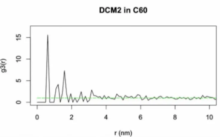
that 10 nm which contained 593 DCM2 molecules. This value is between the 3x3x3 and 4x4x4 sample size simulations in figure 3.3. This subsetted data was then scaled and used to generate a RDF which can be seen in figure 3.8.

It must be noted that the data in the RDF seen in figure 3.8 was scaled. The reason for this scaling is that the reconstruction parameters for an organic sample in the LEAP software are largely unknown. As such there is some error in the reconstructed spatial data which is accounted for with this scaling. It can be seen that there is some small radius below which no molecules can be found due to repulsive Pauli interactions. This distance was found to be much smaller than ex-pected when the unscaled data was used to create an RDF, at about 0.149 nm. The minimum ra-dius we calculated for DCM2 was 0.574 nm and as such the position data was scaled to reflect that length. In addition, the bin width needed to change to reflect this error. To accomplish this the rmax parameter, set to 8 in all of the simulations, was scaled in the same manner as the radial data giving an rmax of 31. This accounted for the error in the reconstruction parameters by

creasing bin width. In the future it may be possible to use the scaling factor to investigate more accurate reconstruction parameters.

The RDF in figure 3.8 mirrors those seen in the simulations especially in shape. There is a large initial peak followed by smaller peaks and small oscillations about one as the data goes further out in r. If the experimental data is compared to the simulated data in figure 3.5 it can be seen that it closely resembles the simulated monomer data in that the initial peak height is on the same order of magnitude. The peak value of the simulated monomers is 7.2 and the peak value of the experimental data seen in figure 3.8 is 15.4. Since the peak value of the simulated dimers was 103.33 the experimental data indicates primarily monomers. However, this does not defini-tively mean that clustering is not present. The fact that this data indicates monomers could be due to a deficiency in the number of points used, since we were aiming for a sample on the order of the 6x6x6 simulation sample size which contained 6 times more data points than were collected, or due to a lack of the simulations or reconstruction parameters taking into account the actual structure of DCM2. DCM2 has a large dipole moment and is approximately planar in structure. This being the case DCM2 is likely to stack, analogous to a deck of cards, rather than creating random clusters as were simulated. Also, if reconstruction parameters are incorrect molecule po-sition could be distorted in some unexpected way.

Overall, the DCM2 in C60 sample provided a good starting point and will be used as com-parison for the next sample tested, 2% DCM2 in Alq3. This sample is more relevant to OLED de-vices as it contains materials typically seen in the emitter layer of dede-vices. The same process for

obtained the data was subsetted in mass and position. The same mass range was used for DCM2 as with the last sample. Alq3 was mass ranged from 458 to 463.5 g/mol. The data was then ranged in space to allow for analysis. The data was ranged from -100 to100 nm in x and y and 1.5 to 21.5 nm in the z direction. It should be noted that since this sample was run to completion it was much thicker. As such a larger area could be subsetted in space and still be cuboid as re-quired by the RDF analysis. The data used for the output RDF was once again scaled to reflect the minimum allowed distance between two DCM2 molecules. However, this scaling was less dramatic than the scaling used in figure 3.8. The scaled RDF can be seen in figure 3.9.

The first note is that the above RDF was generated with more DCM2 data than the one see in figure 3.8. This is because the sample was run to completion. There were 1397 data points in the subset of data used, which is still significantly less than the target sample size. The volume of the subset used was also 50 times bigger than the DCM2 in C60 sample size. It should also be noted that the scaling needed to correct for the minimum distance between two molecules was

much lower than the DCM2 in C60 sample. The distance found in an RDF created with unscaled data was 0.408 nm which was then scaled to 0.574 nm. This scaling factor was also applied to rmax and increased that value from 8 to 11.25 which is a much smaller change than in the previ-ous data set. One of the reasons for the lessor need for scaling is that two reconstructions were made. These reconstructions will be discussed in greater detail in section 3.4. In summary, the first reconstruction was created to have a thickness which matched the deposition thickness. The second reconstruction was further adjusted in order to get more accurate molecular spacing. The second reconstruction was then used for analysis.

This RDF again closely mirrors the shape of those seen in simulations. This RDF has a very high initial peak relative to the rest of the data. After this initial peak we see some small peaks which quickly oscillate to one. This indicates monomers. This initial peak magnitude, at 8.95, closely resembles the peak hight of monomers seen in figure 3.5, even more so than the data seen in figure 3.8. If the peak height were greater arguments could be made for clustering. Again, this does not necessarily mean no clustering is present. The reconstruction parameters could be masking clustering effects by distorting the data. Also, we still need more data points in order to hit the target value. While this data set had more points than the previous one it was still only 37.17% of the target 3700 data points contained in the 6x6x6 simulated data set. Both thicker samples and reconstruction parameters need to be further investigated before clustering may be ruled out.

of the DCM2 in Alq3 sample. This indicates that there is relatively more dimer formation in the C60 sample. This makes sense for a couple reasons. Firstly, the dipole moment of C60 is lower than that of Alq3. This means that C60 is less likely than Alq3 to experience dipole interactions with DCM2 and prevent said DCM2 from creating a dimer with another DCM2 molecule. Sec-ondly, there was a higher relative concentration of DCM2 in the C60 sample which leads to a higher probability of clusters. Also, not including the main peak, there are two smaller peaks seen in the C60 sample RDF. These two smaller peaks occur at radius 1.2 nm and 1.7 nm. These peaks are not seen in the RDF of the Alq3 sample. This again indicates more clustering in that those peaks could result from second nearest neighbors. Finally, the two experimental data sets closely mirror one another in shape, excluding those smaller peaks just mentioned. This is rea-sonable because the RDF is calculated for the same molecule in both graphs and as such it is ex-pected to see similar features in both.

3.4 Investigation of Reconstructions

In order to further investigate the effect of reconstruction parameters on the data sets gen-erated by the LEAP software, two reconstructions which were created for the DCM2 in Alq3 sample were compared. The first reconstruction was created by matching the thickness recorded from the deposition to the thickness of the reconstruction. The second reconstruction was then built off of the first by adjusting the image compression to obtain more accurate molecular sping. The second reconstruction was analyzed because it contained position data which more ac-curately represented the minimum distance between two DCM2 molecules. A histogram of the

concentration of DCM2 molecules in each reconstruction in the x-y plane can be seen in figure 3.10.

The concentration maps seen in figure 3.10 are very similar in appearance. The biggest difference is the scaling in x and y. The axis on the first reconstruction's concentration map ranges from -500 to 500 whereas the axis for the second reconstruction ranges from about -1100 to 1100. Between the two reconstructions the scaling in x and y therefore changed by a factor of ~2. However these concentration maps were created by compressing all of the z data into the x-y plane. When looking at the range of the z data contained in each graph, the scaling only changed by a factor of about 1.3. This means that the reconstructions do not identically scale all three di-mensions. In order to investigate how the reconstructions differed with respect to molecular

from the second reconstruction, eg the RDF which was used to determine the scaling factor that was then applied to the data analyzed in section 3.3, was compared to an RDF of the data from the first reconstruction. Since the dimensions changed in x, y and z between reconstructions there was a need to use a different area for analysis in the first reconstruction than was seen in the sec-ond reconstruction. The area chosen from the first reconstruction was -45 nm to 45 nm in x and y and 1.5 to 51.5 nm in z as compared to the area used from the second reconstruction which was -100 to 100 nm in x and y and 1.5 to 21.5 nm in z. The thickness was increased in the sample from the first reconstruction to obtain approximately the same number of data points analyzed in the second reconstruction. It should be noted that these are unscaled data sets and as such the units are nominally nanometers as that is the unit the LEAP software uses but neither data set was scaled to reflect accurate molecular spacing. The data from the first reconstruction was then scaled to have the same initial peak location in the RDF as the data from the first reconstruction for ease of comparison. The two generated RDF plots can be seen in figure 3.11.

In comparing the two RDF plots depicted in figure 3.11 there are noticeably more peaks near the initial peak in one RDF versus the other. There are two new peaks in the first reconstruc-tion data which were not seen in the second reconstrucreconstruc-tion located at r ~ 0.66 nm and r ~ 0.98 nm. We suggest that these new peaks are caused by the compression in the z direction between the two reconstructions. If data is being compressed non uniformly in one direction, namely the z direction, we would expect to see a splitting of the initial peak because a point which was more distant before the compression would now be close enough to another molecule to constitute a second or third nearest neighbor. In order to implement the correct reconstruction parameters there is a need for some sort of marker in the x-y plane which would allow us to know a distance in that plane. This would allow for the reconstruction to be scaled to accurately reflect that known dimension as well as the known thickness in the z dimension. Until such a time as we have a known distance to scale to in the reconstruction parameters it is difficult to analyze how accurate the reconstructions we are generating truly are.

CHAPTER 4

CONCLUSIONS AND FUTURE WORK

In summary, this work investigated methods for analyzing clustering behavior in OLED emitter layers. First, background information was given to show what is currently known about OLED devices and to discuss loss mechanisms that could be reduced through deeper analysis of OLED structure. Then, simulations were developed in order to aid in the understanding of exper-imental data analysis. These simulations were developed using a random close packed structure. Samples were then made by creating large parent structures and sampling from those the desired concentration as well as accounting for detector efficiency. Simulations were then used to eluci-date the effects of detector efficiency, sample size and cluster size on data analysis. Next, experi-mental data was taken on two systems, 3% DCM2 in C60 and 2% DCM2 in Alq3. This data was first represented as a mass spectrum. Data analysis in the form of RDFs was then implemented. Evidence of clustering was not expressly seen in both samples. While the analysis of experimental data indicated monomers in both systems it is possible that clustering is still present. The re sults presented could be indicative that more data points are needed, better reconstruction param -eters are needed or that the structure of DCM2 was not ideally modeled in the simulations. In this analysis it was also shown that it is possible to create a three dimensional reconstruction of OLED films using LEAP. This is a huge step forward in further understanding the underlying structure and physics of OLED devices.

There are many paths for future work upon completion of this project. The first task is to better define the reconstruction parameters in the LEAP software so that scaling of the data is no

longer necessary. In order to do this there is a need for a marker molecule to be placed in our samples. This marker molecule would need to be one which can be easily deposited in a colum-nar structure to create a grid pattern in the x-y plane of the sample. In knowing the spacing of said grid one could determine reconstruction parameters which accurately recreate this spacing. Once the reconstruction parameters are accurately known, other films should be examined using the same technique. These films could simply be different concentrations of DCM2 in Alq3, other film thicknesses or other materials. Other material systems could include Ir(ppy)3 in CBP or TCTA or DCJMTB in Alq3 as these are commonly seen systems in the literature. Exciton dynam-ics could also be investigated using the LEAP data. If a device was created and a photolumines-cence curve taken this curve could be compared to a histogram of concentrations in the sample to elucidate exciton dynamics. This correlation would be able to show where excitons were relaxing and emitting light, whether that be in the more randomly dispersed locations or in the clusters, should clusters be concretely found in other samples. Finally, better OLED devices could be cre-ated once the structural information as well as the light emission location was better understood.

REFERENCES CITED

[1] C. Denison, “OLED vs. LED: Which is the better TV technology?,” Digital Trends. [On-line]. Available: http://www.digitaltrends.com/home-theater/oled-vs-led-which-is-the-better-tv-technology/. [Accessed: 10-Aug-2015].

[2] B. Robinson, “OLED vs LED Lighting,” http://blog.1000bulbs.com/. [Online]. Available: http://blog.1000bulbs.com/oled-vs-led-lighting/. [Accessed: 26-Aug-2015].

[3] “Universal Display Corporation.” [Online]. Available: http://www.udcoled.com/default-.asp?contentID=604. [Accessed: 27-Sep-2015].

[4] A. Laaperi, “OLED lifetime issues from a mobile-phone-industry point of view,” J. Soc. Inf. Disp., vol. 16, no. 11, pp. 1125–1130, Nov. 2008.

[5] “LED/Fluorescent/Incandescent Efficacy Table,” Designing with LEDs. [6] “OLED Basics | Department of Energy.” [Online]. Available:

http://energy.gov/eere/ssl/oled-basics. [Accessed: 26-Aug-2015].

[7] Q. Wang, I. W. H. Oswald, M. R. Perez, H. Jia, B. E. Gnade, and M. A. Omary, “Exciton and Polaron Quenching in Doping-Free Phosphorescent Organic Light-Emitting Diodes from a Pt(II)-Based Fast Phosphor,” Adv. Funct. Mater., vol. 23, no. 43, pp. 5420–5428, Nov. 2013.

[8] G. S. Sebastian Reineke, “Highly phosphorescent organic mixed films: The effect of ag-gregation on triplet-triplet annihilation,” Appl. Phys. Lett., vol. 94, no. 16, pp. 163305– 163305–3, 2009.

[9] Electrical Engineering Department: Technion, “Organic Semiconductors and Devices: Excitons.” 1999.

[10] H. Yersin and W. J. Finkenzeller, “Triplet Emitters for Organic Light-Emitting Diodes: Basic Properties,” in Highly Efficient OLEDs with Phosphorescent Materials, H. Yersin, Ed. Wiley-VCH Verlag GmbH & Co. KGaA, 2007, pp. 1–97.

[11] “Calculate Resonance Energy Transfer (FRET) Efficiencies - The fluorescence labora-tory.” [Online]. Available:

http://www.fluortools.com/software/ae/documentation/tools/FRET. [Accessed: 31-Aug-2015].

[12] “Critical Transfer Distance Determination Between FRET Pairs.” [Online]. Available: http://www.photobiology.info/Experiments/Biolum-Expt.html. [Accessed: 27-Sep-2015]. [13] “Dexter Energy Transfer.” [Online]. Available:

http://chemwiki.ucdavis.edu/Theoretical_Chemistry/Fundamentals/Dexter_Energy_Transfer . [Accessed: 31-Aug-2015].

[14] A. P. Demchenko, Advanced Fluorescence Reporters in Chemistry and Biology II: Molecular Constructions, Polymers and Nanoparticles. Springer Science & Business Media, 2010.

[15] Y. H. Park, Y. Kim, H. Sohn, and K.-S. An, “Concentration quenching effect of organic light-emitting devices using DCM1-doped tetraphenylgermole,” J. Phys. Org. Chem., vol. 25, no. 3, pp. 207–210, Mar. 2012.

[16] R. Farchioni and G. Grosso, Organic Electronic Materials: Conjugated Polymers and Low Molecular Weight Organic Solids. Springer Science & Business Media, 2013.

[17] P. Schouwink, A. H. Schäfer, C. Seidel, and H. Fuchs, “The influence of molecular aggre-gation on the device properties of organic light emitting diodes,” Thin Solid Films, vol. 372, no. 1–2, pp. 163–168, Sep. 2000.

[18] Y. Divayana and X. W. Sun, “Observation of Excitonic Quenching by Long-Range Dipole-Dipole Interaction in Sequentially Doped Organic Phosphorescent Host-Guest Sys-tem,” Phys. Rev. Lett., vol. 99, no. 14, p. 143003, Oct. 2007.

[19] S. Reineke, G. Schwartz, K. Walzer, M. Falke, and K. Leo, “Highly phosphorescent or-ganic mixed films: The effect of aggregation on triplet-triplet annihilation,” Appl. Phys. Lett., vol. 94, no. 16, p. 163305, Apr. 2009.

[20] M. A. Baldo, Z. G. Soos, and S. R. Forrest, “Local order in amorphous organic molecular thin films,” Chem. Phys. Lett., vol. 347, no. 4–6, pp. 297–303, Oct. 2001.

[21] J.-R. Gong, L.-J. Wan, S.-B. Lei, C.-L. Bai, X.-H. Zhang, and S.-T. Lee, “Direct Evidence of Molecular Aggregation and Degradation Mechanism of Organic Light-Emitting Diodes under Joule Heating:  an STM and Photoluminescence Study,” J. Phys. Chem. B, vol. 109, no. 5, pp. 1675–1682, Feb. 2005.

[22] A. R. G. Smith, J. L. Ruggles, H. Cavaye, P. E. Shaw, T. A. Darwish, M. James, I. R. Gentle, and P. L. Burn, “Investigating Morphology and Stability of Fac-tris

(2-[23] G. L. Ingram and Z.-H. Lu, “Design principles for highly efficient organic light-emitting diodes,” J. Photonics Energy, vol. 4, no. 1, pp. 040993–040993, 2014.

[24] Y. Q. Zhang, G. Y. Zhong, and X. A. Cao, “Concentration quenching of electrolumines-cence in neat Ir(ppy)3 organic light-emitting diodes,” J. Appl. Phys., vol. 108, no. 8, p. 083107, Oct. 2010.

[25] N. C. Giebink and S. R. Forrest, “Quantum efficiency roll-off at high brightness in fluo-rescent and phosphofluo-rescent organic light emitting diodes,” Phys. Rev. B, vol. 77, no. 23, p. 235215, Jun. 2008.

[26] J. S. Price and N. C. Giebink, “Quantum efficiency harmonic analysis of exciton annihi-lation in organic light emitting diodes,” Appl. Phys. Lett., vol. 106, no. 26, p. 263302, Jun. 2015.

[27] C. W. Tang, S. A. VanSlyke, and C. H. Chen, “Electroluminescence of doped organic thin films,” J. Appl. Phys., vol. 65, no. 9, pp. 3610–3616, May 1989.

[28] B. Chen, X. Lin, L. Cheng, C. Lee, W. A. Gambling, and S. Lee, “Improvement of effi-ciency and colour purity of red-dopant organic light-emitting diodes by energy levels match-ing with the host materials,” J. Phys. Appl. Phys., vol. 34, no. 1, p. 30, 2001.

[29] J. L. Yarnell, M. J. Katz, R. G. Wenzel, and S. H. Koenig, “Structure Factor and Radial Distribution Function for Liquid Argon at 85K,” Phys. Rev. A, vol. 7, no. 6, pp. 2130–2144, Jun. 1973.

[30] “Kenneth Desmond Physics Home Page.” [Online]. Available: http://www.engineer-ing.ucsb.edu/~kdesmond/Algorithms.html. [Accessed: 31-Mar-2016].

[31] E. W. Weisstein, “Random Close Packing.” [Online]. Available: http://mathworld.wol-fram.com/RandomClosePacking.html. [Accessed: 11-Mar-2016].

APPENDIX A

The following is annotated code which allows for reproduction of section 3.1 simulations. Any of the comments which mention a function from the rapt-file.R package or the rapt-sim.R package were created by Andrew Proudian, as mentioned in the acknowledgments. The follow-ing section is formatted such that, if the rapt-file.R and rapt-sim.R packages are loaded, the text can be copied and pasted into a script file in R. This script can then be run to generate one of the simulations discussed in this work.

# First the building block generated by the RCP generator is imported and scaled so that the ra-dius of each molecule is 0.5 units.

rcp.3000 <- (.5/.369027)*read.table('~/Documents/thesis/Simulated_data/rcpgenerator/ 3000_point/FinConfig23', header = TRUE, sep = "")

# The above table is now turned into a pp3, or three dimensional point pattern, using a function from rapt-file.R.

rcp.3000.pp3 <- createSpat(rcp.3000, win = NULL)

# The building block is now tessellated to make a 3x3x3 parent sample. The function shift.pp3, from the rapt-sim.R package, is an extension of the built in shift function. The difference being the shift cannot handle pp3 class, i.e. 3 dimensional, objects where as shift.pp3 can.

# Shift is used twice in the x direction

rcp.3000.x1 <- shift.pp3(rcp.3000.pp3, vec = c(13.54, 0, 0), origin = NULL) rcp.3000.x2 <- shift.pp3(rcp.3000.x1, vec = c(13.54, 0, 0), origin = NULL)

# Now superimpose.pp3 from the rapt-sim.R package, an analogous extension of the superim-pose function, is used to piece together the three blocks that have been created in the x direction. rcp.3000.x.3 <- superimpose.pp3(rcp.3000.pp3, rcp.3000.x1, rcp.3000.x2, W= NULL, check = F)

# This process is repeated for the y and z direction until the final product, rcp.3000.3, has been created.

rcp.3000.y1.3 <- shift.pp3(rcp.3000.x.3, vec = c(0, 13.54, 0), origin = NULL) rcp.3000.y2.3 <- shift.pp3(rcp.3000.y1.3, vec = c(0, 13.54, 0), origin = NULL)

rcp.3000.y.3 <- superimpose.pp3(rcp.3000.x.3, rcp.3000.y1.3,rcp.3000.y2.3, W =NULL, check = F)

rcp.3000.z1.3 <- shift.pp3(rcp.3000.y.3, vec = c(0, 0, 13.54), origin = NULL) rcp.3000.z2.3 <- shift.pp3(rcp.3000.z1.3, vec = c(0, 0, 13.54), origin = NULL)

rcp.3000.3 <- superimpose.pp3(rcp.3000.y.3, rcp.3000.z1.3,rcp.3000.z2.3, W =NULL, check = F)

# Now the sample.pp3 function from rapt-sim.R, another extension of the built in sample func-tion designed to handle pp3 class objects, is used to randomly sample 0.5% of the points in the parent sample.

rcp.3000.3.405 <- sample.pp3(rcp.3000.3, 405)

# Next dimers are created using the nmers function from rapt-sim.R. This function compares the sampled data set to the parent data set and finds the next nearest neighbor (n=2) from the parent

sample for the points in the sampled data set. It outputs a new pp3 class object which contains both the original points and the nearest neighbors.

rcp.3000.3.dimers <- nmers(rcp.3000.3.405, rcp.3000.3, n=2)

# The sample function is now used again to sample 58% of the points in the dimer data set. rcp.3000.3.dimers.58 <- sample.pp3(rcp.3000.3.dimers, 470)

# Now a RDF is created using pcf3est. In pcf3est delta is the half-width of the smoothing kernel, rmax is the maximum value of r for which the RDF will be calculated, nrval is number of values of r for which the RDF will be calculated and biascorrect is a correction for the value of the smoothing kernel at r=0.

rcp.3000.3.dimers.58.pcf <- pcf3est(rcp.3000.3.dimers.58, delta = .05, rmax = 8, nrval = 256, bi-ascorrect = F)

# A plot is then created. This is the blue line seen in figure 7.

plot(rcp.3000.3.dimers.58.pcf, log = "y", xlim = c(.8 , 4), ylim = c(.1, 100), lwd = 2.5, col = "blue", legend = FALSE, main = DIMERS)