3-D GEOLOGIC MODEL OF THE LEWIS SHALE IN THE GREAT DIVIDE AND WASHAKIE BASINS,
WYOMING
by
(Geology) Golden, Colorado Date ______________ Signed: ______________________ Doddy Suryanto Approved: ____________________ Dr. Neil F. Hurley Thesis Advisor Golden, Colorado Date ______________ ______________________ Dr. Murray Hitzman
Professor and Head,
Department of Geology and
Geological Engineering
ABSTRACT
The Lewis Shale is an emerging natural gas exploration target in the Great Divide
and Washakie basins, Wyoming. The purpose of this study is to estimate the volumes of
gas-in-place in the Lewis Shale interval. This study employs a 3-D geologic model and
uses this information to calculate gas-in-place volumes in sandstone lobes of the Lewis
Shale.
Cross sections were constructed across the study area prior to doing regional
stratigraphic correlation. Using this technique, 12 sandstone lobes were interpreted.
Different inferred paleocurrent directions were also interpreted using isopach maps.
Deep-water sandstones of the Lewis Shale initially entered from the northwest and later
from the northeast, southwest and east.
A 3-D geologic model was built to mimic the subsurface geology of the Lewis
Shale in the Great Divide and Washakie basins. Well log data, a 3-D geologic model, and
a 3-D porosity model were integrated to calculate gas-in-place volumes in each sandstone
lobe. Using the correlation scheme of this study, the Orange Sand was interpreted to be
the sand that holds the largest gas-in-place volume. The Blue Sand holds the second
largest gas-in-place volume. Both of these sands occur in the Dad Member of the middle
Lewis Shale. Because of the vast lateral extent of the Orange and Blue Sands, they hold
the largest gas-in-place volume.
hydrocarbon saturations used in calculations are 40%, 50%, and 60%. Temperature data
for each sandstone lobe were calculated by multiplying the midpoint depth of each
sandstone lobe by a temperature gradient of 1.5o F/100 ft. Pressure data for each
sandstone lobe were calculated by multiplying the midpoint depth of each sandstone lobe
by the pressure gradient. Two pressure gradients were used to calculate gas-in-place
volumes. A pressure gradient of 0.45 psi/ft was used for sand above the top of
overpressure. Pressure gradient of 0.65 psi/ft was used for sand below the top of
overpressure. Volumetric calculations using average porosity showed that gas-in-place
volumes range from 62.2 to 82.9 Tcf. Volumetric calculations using porosity as a
function of depth showed that gas-in-place volumes range from 46.5 to 62.0 Tcf. The
volume difference calculated between both calculations was 25.2%. This indicates that
estimated hydrocarbon volume decreases with increased sophistication of porosity
modeling.
In this study, the estimates of gas-in-place volumes are substantially less than
previous estimates. It should be noted that the previous estimates covered the entire
Greater Green River basin, whereas this study focuses on part of the Eastern Greater
Green River basin. The estimates of gas-in-place volumes are one-twelfth compared to
the estimates of gas-in-place volumes calculated by Law et al. (1989) for all reservoirs in
the Lewis Shale in the entire Greater Green River basin.
TABLE OF CONTENTS
ABSTRACT………... iii
LIST OF FIGURES………... x
LIST OF TABLES………. xiv
ACKNOWLEDGEMENTS……….. xv DEDICATION………... xvi CHAPTER 1. INTRODUCTION……… 1 1.1. Introduction………. 1 1.2. Research Objectives……… 1 1.3. Research Methods………... 2 1.4. Research Contributions………... 5 1.5. Previous Work……… 6
CHAPTER 2. GEOLOGICAL SETTING……….. 9
2.1. Location of Study Area………... 9
2.2. Stratigraphy………. 12 2.2.1. Regional Stratigraphy………. 12 2.2.2. Local Stratigraphy………... 18 2.3. Tectonics………. 23 2.3.1. Regional Tectonics……….……….23 2.3.2. Local Tectonics………... 29 2.4. Petroleum Geology………. 32 2.5. Petroleum System……… 38 v
2.5.3. Seal Rock……… 40
2.5.4. Overburden Rock……… 41
2.5.5. Hydrocarbon Generation, Expulsion, and Migration……….…………. 41
CHAPTER 3. SUBSURFACE INTERPRETATION……….… 44
3.1. Introduction………. 44
3.2. Previous Work………. 44
3.2.1. Cross Sections from Lee Shannon………….………. 48
3.2.2. Cross Section from Pyles (2000)……… 50
3.2.3. Cross Sections from Hamzah (2001)……….………. 53
3.3. Data Set………61
3.3.1. Digital Data………. 61
3.3.2. Cross Section Data Set……… 61
3.4. Correlation………... 65
3.5. Cross Section Interpretation……… 66
3.5.1. North-South Cross Sections……… 67
3.5.2. East-West Cross Sections………... 68
3.6. Structure Maps……… 71
3.6.1. Top of the Mesaverde………. 71
3.6.2. Top of the Asquith marker……….. 75
3.6.3. Top of the Lewis Shale………... 75
3.7. Isopach Maps……….. 75
3.7.1. Olive Green Sand……… 78
3.7.2. Red Sand………. 78
3.7.3. Gold Sand………... 80
3.7.4. Orange Sand……… 80
3.7.5. Dark Green Sand………. 84
3.7.6. Dark Red Sand……… 84
3.7.7. Yellow Sand……… 84
3.7.8. Blue Sand……… 87
3.7.9. Brown Sand……….……… 87
3.7.10. Light Green Sand……… 91
3.7.11. Purple Sand………. 91
3.7.12. Light Blue Sand……….. 91
3.8. Discussion………... 94
CHAPTER 4. OVERPRESSURE……… 101
4.1. Background………. 101
4.2. Overpressure Mechanisms……….. 101
4.2.1. Stress-Related Overpressure………... 101
4.2.1.1. Vertical Stress-Related Overpressure……… 102
4.2.1.2. Lateral/Horizontal Stress-Related Overpressure……… 103
4.2.2. Fluid Volume Increase……… 104
4.2.2.1. Aquathermal Expansion………. 104
4.2.2.2. Mineral Transformation………. 104
4.2.2.3. Hydrocarbon Generation……… 105
4.3. Data………. 107
4.4. Overpressure Interpretation………. 109
4.5. Overpressure Generation in the Great Divide and Washakie basins…………...114
4.6. Discussion………... 122
5.2.1. Stratigraphic Framework……… 136 5.2.1.1. Horizon Modeling……….. 137 5.2.1.2. Creation of Zones………... 138 5.2.1.3. Creation of 3-D Grids………. 139 5.2.2. Blocking Wells………143 5.2.3. Lithology Modeling……… 144 5.2.4. Petrophysical Modeling……….. 150 5.3. Data………. 151 5.3.1. Stratigraphic Data………... 151 5.3.2. Petrophysical Data……….. 151 5.4. Interpretation………... 156
5.4.1. Gamma Ray Distribution……… 156
5.4.2. Sandstone Distribution……… 171
5.4.3. Porosity Distribution………... 172
5.5. Validation of Cross sections………. 173
5.6. Discussion……… 176
CHAPTER 6. VOLUMETRIC CALCULATIONS AND ECONOMIC CONSIDERATIONS………. 179 6.1. Volumetric Calculations……….. 179 6.1.1. Sand Volumes………. 181 6.1.2. Pore Volumes……….. 184 6.1.3. Gas-In-Place Volumes……… 189 6.2. Economic Considerations……… 200 6.3. Discussion………... 201 viii
CHAPTER 7. CONCLUSIONS AND RECOMMENDATIONS……….. 208
7.1. Conclusions………. 208
7.2. Recommendations………... 210
REFERENCES……….. 211
APPENDICES……… 225
Appendix A. Log tops………. 226
Appendix B. List of wells for overpressure interpretation……….. 245
Appendix C. List of wells for normalization………... 251
Appendix D. List of wells for core analyses………... 253
Files and data are included in electronic format in the CD ROM at the back of the thesis.
Figure Page
Figure 2.1. Location of the study area……….. 10
Figure 2.2. Map of major tectonic features………... 11
Figure 2.3. Regional stratigraphic column in south-central Wyoming………. 13
Figure 2.4. Depositional environment model ………...…….……….. 16
Figure 2.5. Type log of the Lewis Shale interval in the Washakie basin…………. 19
Figure 2.6. Channel and sheet sandstone of the Dad Sandstone member…………21
Figure 2.7. Inferred directions of delta progradation………... 24
Figure 2.8. Western Interior Seaway……… 27
Figure 2.9. Paleogeographic map of the Cordilleran highlands……….…..28
Figure 2.10. Stratigraphic cross section of the Lost Soldier anticline………... 31
Figure 2.11. Total producing wells for the Lewis Shale play……… 34
Figure 2.12. Map of the Lewis Shale production fields……… 37
Figure 3.1. Cross section data set from previous work……… 45
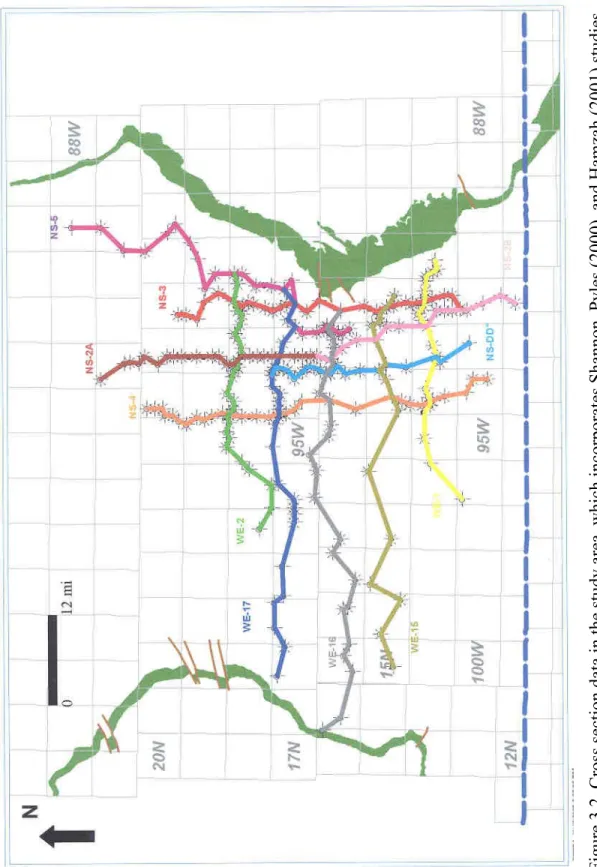
Figure 3.2. Cross section data set from Shannon, Pyles (2000), and Hamzah (2001)………... 47
Figure 3.3. Composite log of the Lewis Shale in the Hay Reservoir….…………..49
Figure 3.4. Map of Pyles (2000) cross section……….51
Figure 3.5. High-resolution stratigraphic cross section of the Lewis Shale……… 52
Figure 3.6. Progradation pattern of sandstone lobes in the N-S cross section……. 54
Figure 3.7. Lateral shift of sandstone lobes in the W-E cross section………. 55
Figure 3.8. Sandstone lobes color scheme………... 56
Figure 3.9. Hamzah (2001) isopach map of the Red Sand ………. 57
Figure 3.10. Source directions of Hamzah’s (2001) Olive Green, Red, Gold, and
Orange Sands……… 58
Figure 3.11. Source directions of Hamzah’s (2001) Dark Green, Dark Red, Blue, and Brown Sands……….. 59
Figure 3.12. Source directions of Hamzah’s (2001) Light Green, Purple, and Light Blue Sands……… 60
Figure 3.13. Digital log data………. 62
Figure 3.14. Cross section data set………64
Figure 3.15. Cross Section NS-3……….. 69
Figure 3.16. Cross Section WE-1………. 72
Figure 3.17. Cross Section WE-15………... 73
Figure 3.18. Structure map on top of the Mesaverde……… 74
Figure 3.19. Structure map on top of the Asquith marker ………... 76
Figure 3.20. Structure map on top of the Lewis Shale………..77
Figure 3.21. Isopach map of the Olive Green Sand……….. 79
Figure 3.22. Isopach map of the Red Sand………... 81
Figure 3.23. Isopach map of the Gold Sand………. 82
Figure 3.24. Isopach map of the Orange Sand………. 83
Figure 3.25. Isopach map of the Dark Green Sand……….……….. 85
Figure 3.26. Isopach map of the Dark Red Sand……….. 86
Figure 3.27. Isopach map of the Yellow Sand……….. 88
Figure 3.28. Isopach map of the Blue Sand……….. 89
Figure 3.29. Isopach map of the Brown Sand……….………….. 90
Figure 3.30. Isopach map of the Light Green Sand……….…………. 92
Figure 3.31. Isopach map of the Purple Sand………... 93
Figure 3.32. Isopach map of the Light Blue Sand……… 95
Figure 3.33. Typical log signature in channel lobe complex system……… 99
Figure 3.34. Typical log responses in cross section NS-2A………. 100
Figure 4.4. Barrett Resources Corporation Rulison No.1 Deep well………. 111
Figure 4.5. Plot of velocity versus depth……… 113
Figure 4.6. Pressure profile for wells in the Pacific Creek area………. 115
Figure 4.7. Rapid increase in total gas indicates overpressure………... 119
Figure 4.8. Rapid increase in mud weight indicates overpressure………. 120
Figure 4.9. Log responses in the overpressure zone………... 121
Figure 4.10. Map of tops of overpressure in measured depth………... 123
Figure 4.11. Map of tops of overpressure in subsea depth………... 124
Figure 4.12. Structural cross section WE-17 ………... 125
Figure 4.13. Structural cross section NS-4………... 126
Figure 4.14. Log responses for the Windmill Draw #2 well ………... 127
Figure 4.15. Plot of percent illite in mixed-layer illite/smectite (I/S) clays versus depth……….. 128
Figure 4.16. Mud weight responses for the Frewen Deep #1 well………... 129
Figure 4.17. Potentiometric surface map……….. 131
Figure 4.18. Map of isoresistivity………. 132
Figure 5.1. Two 3-D grid types……….. 140
Figure 5.2. Constant cell thickness………. 142
Figure 5.3. Constant number of layers……… 142
Figure 5.4. Location of reference wells used for normalization………. 146
Figure 5.5. Normalization of GR curves………. 148
Figure 5.6. Pre-normalized and normalized GR curves……….. 149
Figure 5.7. Surfaces data………. 152
Figure 5.8. Distribution of porosity data ……… 154
Figure 5.9. Normal distribution of porosity data……… 155
Figure 5.10. 3-D GR model of the Lewis Shale………157
Figure 5.11. 3-D porosity model of the Lewis Shale……… 158
Figure 5.12. 3-D geologic model of the Olive Green Sand……….. 159
Figure 5.13. 3-D geologic model of the Red Sand………... 160
Figure 5.14. 3-D geologic model of the Gold Sand……….. 161
Figure 5.15. 3-D geologic model of the Orange Sand……….. 162
Figure 5.16. 3-D geologic model of the Dark Green Sand………... 163
Figure 5.17. 3-D geologic model of the Dark Red Sand……….. 164
Figure 5.18. 3-D geologic model of the Yellow Sand……….. 165
Figure 5.19. 3-D geologic model of the Blue Sand……….. 166
Figure 5.20. 3-D geologic model of the Brown Sand………... 167
Figure 5.21. 3-D geologic model of the Light Green Sand……….. 168
Figure 5.22. 3-D geologic model of the Purple Sand………... 169
Figure 5.23. 3-D geologic model of the Light Blue Sand……… 170
Figure 5.24. Validation of Cross Section NS-4………. 174
Figure 5.25. Validation of Cross Section NS-5………. 175
Figure 5.26. Validation of Cross Section WE-17……….. 177
Figure 6.1. Distribution of the top of overpressure……… 180
Figure 6.2. Distribution of net sand volumes in the Orange Sand……….. 183
Figure 6.3. Distribution of pore volumes in the Orange Sand……… 186
Figure 6.4. Distribution of gas-in-place volumes calculated using average porosity and 60% hydrocarbon saturation………... 202
Figure 6.5. Distribution of gas-in-place volumes calculated using porosity as a function of depth and 60% hydrocarbon saturation…… 203
Figure 6.6. Distribution of total gas-in-place volumes calculated using average porosity and different hydrocarbon saturations……….. 204
Figure 6.7. Distribution of total gas-in-place volumes calculated using porosity as a function of depth and different hydrocarbon saturation.. 205
Table Page
Table 2.1. Various estimates of gas resources in the Greater Green River basin… 33 Table 2.2. Gas resources of the Lewis Shale………... 35 Table 2.3. Events chart of the Lewis Shale petroleum system……… 43 Table 4.1. Attributes of direct and indirect basin-centered gas systems…………. 117 Table 6.1. Distribution of sand volumes ………. 182 Table 6.2. Distribution of pore volumes calculated using average porosity………185 Table 6.3. Distribution of pore volumes calculated using porosity
as a function of depth………. 188 Table 6.4. Distribution of gas-in-place volumes calculated using average
porosity and 45% hydrocarbon saturation……….. 190 Table 6.5. Distribution of gas-in-place volumes calculated using average
porosity and 50% hydrocarbon saturation……….. 191 Table 6.6. Distribution of gas-in-place volumes calculated using average
porosity and 60% hydrocarbon saturation……….. 192 Table 6.7. The midpoint, temperature, and pressure data for each sandstone lobe
in the Lewis Shale……….. 194 Table 6.8. Distribution of gas-in-place volumes calculated using porosity
as a function of depth and 45% hydrocarbon saturation……… 197 Table 6.9. Distribution of gas-in-place volumes calculated using porosity
as a function of depth and 50% hydrocarbon saturation……… 198 Table 6.10. Distribution of gas-in-place volumes calculated using porosity
as a function of depth and 60% hydrocarbon saturation……… 199
ACKNOWLEDGMENTS
I would like to acknowledge Dr. Neil F. Hurley for allowing me to participate in
the Lewis Shale Project Phase II. I also thank him for his time, patience, guidance, and
discussion dedicated to supervise this study. I would like to thank Dr. John B. Curtis for
valuable discussions. I thank Dr. Geoffrey Thyne and Dr. Matthew Pranter for their
suggestions and comments during the completion of this thesis. Their suggestions,
comments and reviews of the manuscript of this thesis were of immeasurable help.
I would like to express my appreciation to Dr. Michael H. Gardner for giving me
the RMS license and to Safian Atan for teaching me RMS software and for sharing his
knowledge and experience. I would like to thank Ira Pasternack for teaching me PETRA
software, for dedicating his time to the Lewis Shale Project, and for valuable discussions.
I thank Charlie Rourke for sharing valuable time and for always cheering me up.
I gratefully acknowledge Pertamina for giving me the opportunity and financial
support throughout my study. I also acknowledge the American Association of Petroleum
Geologists (AAPG) and Society of Professional Well Log Analysts (SPWLA) for
financial support in the form of a student research grant.
I would like to express my gratitude to my friends Bob Adibrata, Ron Tingook,
Jennifer White, Rafael Sanguinetti, Thais Guirigay, Greg Minton, Carlos Moita, and
Alejandro Franco for their thoughts, criticism, and moral support. I would also like to
express my gratitude to my Indonesian friends for their time and moral support.
My parents, Eddy Suryanto and Lilik Sundari,
My parents in law, Muhammad Djaini and Sari Lira,
My brother, Arry Suryanto
and to
My lovely wife Erviani Indah and daughter Shafira Putri Colderia,
who always have a smile to share, love to give, time to spare, a hand to hold and
understanding during the dark and light moments in completing the manuscript.
1
CHAPTER 1 INTRODUCTION
1.1 Introduction
The Lewis Shale is an emerging natural gas exploration target in the Great Divide
and Washakie basins, Wyoming. This study involves the construction of a 3-D geologic
model based on a regional log-correlation framework to help determine the geometry and
volumetric size of the Lewis Shale sandstone reservoirs. This study is needed in order to
make improved estimates of gas-in-place.
1.2 Research Objectives
The ultimate objective of this research is to calculate the volumes of gas-in-place
in the Lewis Shale interval. In order to achieve this objective, the study employs a 3-D
geologic model, which is based on a subsurface interpretation of well-log data. The
purpose of subsurface interpretation is to identify the geometry and distribution of
sandstone bodies that lie within the Lewis Shale in the Great Divide and Washakie basins
of Wyoming. The other objectives of this study are:
• Construct a stratigraphic framework based on well-log data previously interpreted.
• Construct a 3-D geologic model of the sandstone lobes of the Lewis Shale using the 3-D modeling software RMS (Reservoir Modeling System).
• Calculate sand volume in each sandstone lobe using a gamma ray cutoff. • Calculate pore volumes using a constant value of porosity and a porosity versus
depth function developed from core analyses.
• Calculate gas-in-place volumes using different hydrocarbon saturations and constrained pressure by the top of overpressure.
1.3 Research Methods
Research methods include subsurface data set preparation, subsurface analysis,
computer modeling and volumetric calculation. The ultimate output, a 3-D geologic
model, was constructed using log correlations in regional cross sections. Subsequently,
this model was utilized in the calculation of Lewis Shale gas-in-place volumes in the
Great Divide and Washakie basins. The research methods are:
• Load data set
The data set, which includes the base map, described core, well location,
and well log data for 232 wells were loaded into PETRA software. The locations
of subsurface data points are very important in order to build a 3-D geologic
3
• Edit data set
Digital data need to be edited prior to doing volumetric calculations.
Calibration and digitization processes need to be applied for wells that do not
have digital data. Normalization needs to be applied to all wells drilled in the
study area because of different environments and different service companies.
The normalization work was done using a multi-well histogram approach. The
software used to normalize wells is Power Log. The Creston SE #5 (T19N R91W
Sec. 1) was the well used to determine the gamma ray cutoff for sandstone in the
Lewis Shale interval. The gamma ray cut off was determined by observing the
contact in core between shale and sandstone at the depth of 8,200 ft (2,733 m).
• Well log correlation
As subsurface data types become more sophisticated, a new interpretation
using well log data of the Lewis Shale is developed. The well log data of 232
wells consists of gamma ray, resistivity, sonic, density, and neutron logs. These
well logs were used to interpret the subsurface geology of the Lewis Shale. The
Asquith marker was used as a datum for stratigraphic correlation. Shales above
and below sandstones were used as control markers.
• Overpressure interpretation
Because the overpressure in the study area is caused by gas generation
(Spencer, 1987), the approach is to use several data sets including the sonic and
overpressure is characterized by high sonic transit time and high resistivity
readings. High sonic transit time readings may be caused by the replacement of
lower transit time pore water with higher transit time gas. It may also be caused
by elevated porosity due to reduced compaction. Resistivity increases may be
caused by the replacement of conductive pore water with non-conductive
hydrocarbons.
• Build a 3-D geologic model
After the data were loaded into PETRA, a 3-D geologic model was
developed. The software used to generate the model is RMS (Reservoir Modeling
System). This software interpolates the input data points to generate the surfaces.
The accuracy of the model is based on the density of the data points. The more
data points that we have, the more accurate the model that we generate. The
following steps need to be done prior to building a 3-D geologic model:
1. Build the stratigraphic framework
The stratigraphic framework was built using the interpretation of 11
cross sections. The log tops from 12 sandstone lobes were exported and used
as surfaces. This is the most important step in 3-D modeling. If the
stratigraphic framework is too limited, or is based on an incorrect stratigraphic
interpretation, the resultant 3-D distribution of data can be wrong. Therefore,
it is critical to interpret the stratigraphic framework accurately and with
5
2. Generate facies modeling
Facies modeling was done using gamma ray log and core data. Core
data available for this purpose is from Pyles (2000). A gamma ray cutoff was
applied following the approach of Zainal (2001). This cutoff differentiates
sand from shale using normalized gamma ray logs.
3. Map the top of overpressure
• Volumetric analysis of reservoirs
After a 3-D geologic model is developed, the volumetric analysis can be
done. Sand volumes in each interval were computed after applying the GR cutoff.
Pore volumes were computed using: (1) a constant value of porosity, and (2) a
porosity vs. depth function developed from core analyses. Gas volumes were
computed using different values of water saturation. Pressures were constrained
by the top of overpressure map.
1.4 Research Contributions
Even though the Lewis Shale has been studied for several years and has been the
subject of numerous surface and subsurface studies, there are many things that still need
to be understood. This study is significant because it provides valuable research benefits
regarding a basin-scale 3-D geologic model. Accomplishment of research objectives
contributes to the development of the Lewis Shale. The contribution of this study are
• The well log data were used to map surfaces. These surfaces represent the top and the base of sandstone lobes. The output of mapping surfaces is to develop a
regional stratigraphic framework for the 3-D geologic model.
• The tops of overpressure zones were interpreted using sonic and resistivity logs in addition to pressure, mud weight, and total gas data. An overpressure map
provides information about the distribution of overpressure zones that is very
important for drilling and development programs.
• The 3-D geologic model provides a better way to calculate the volumes of reservoirs. In addition, a 3-D geologic model can be used to generate a flow
simulation model.
• Volumetric calculations were done using different parameters such as gamma ray cutoff, porosity, water saturation, and pressure. The output of the volumetric
calculation is various volume estimations in different sandstone lobes.
1.5 Previous Work
Law et al. (1989) estimated gas resources in Cretaceous and Tertiary sandstone
reservoirs in the Greater Green River basin, Wyoming, Colorado, and Utah. They
estimated that total recoverable gas ranges from 27 to 148 Tcf with 73 Tcf as the mean
estimate for the current technology case, and from 189 to 816 Tcf with 433 Tcf as the
7
tight gas reservoirs associated with overpressure. They have low porosity due to
alteration by deep burial cementation and other factors.
McMillen and Winn (1991) studied sequence stratigraphy and reported that the
Lewis Shale in south-central Wyoming was deposited as a third-order depositional
sequence. They considered the lower part of the Lewis Shale to be the transgressive
systems tract deposits; the Dad Sandstone and the upper part of the Lewis Shale were the
highstand systems tract deposits.
Doelger and Barlow (1997) reported that approximately 85 percent of the total gas
supply in the Greater Green River basin (GGRB) comes from the Lewis Shale, the
Mesaverde Group, the Frontier Formation, and the Muddy-Dakota Formation. However,
only 0.6 Tcf of gas, or 6 percent of its 10.7 Tcf gas resource, has been produced from the
Lewis Shale.
Surdam (1997) reported that Cretaceous shales in the Rocky Mountain Laramide
basins are overpressured. Sandstone bodies within the overpressured shale section are
subdivided stratigraphically and diagenetically into relatively small, isolated,
gas-saturated, and anomalously pressured compartments. In terms of overpressure
mechanism, he interpreted that hydrocarbon generation may be one of the most
potentially effective mechanisms for generating pressure anomalies and pressure
compartmentalization in sedimentary basins.
Witton (1999) worked in the southern Washakie basin. She characterized turbidite
identified two different types of sandstone. Sheet sandstones, which she called lithofacies
A, tend to be laterally continuous. Channel sandstones, which she called lithofacies B,
tend to be laterally discontinuous.
Pyles (2000) interpreted the high-frequency sequence stratigraphy of the Lewis
Shale and Fox Hills Formation in the Great Divide and Washakie basins. He constructed
a 45 mi (72 km) long dip-oriented cross section and recognized two different depositional
patterns. The depositional pattern of the lower part, below a regional shale termed the
Asquith marker, exhibits a retrogradational stacking pattern. The depositional pattern
above the Asquith marker exhibits a progradational stacking pattern. This was interpreted
as a third-order highstand systems tract, which indicated that the Lewis sea regressed
from north to south.
Hamzah (2001) developed regional subsurface correlations of the Lewis Shale in
the Great Divide and Washakie basins using 11 cross sections. In the cross sections, a
prograding stacking pattern was identified from north to south. She also identified 13
sandstone lobes in the Lewis Shale. The distribution of sandstone bodies exhibited lateral
shifts of sandstone depocenters. Six major source directions were interpreted based on the
9
CHAPTER 2
GEOLOGICAL SETTING
2.1 Location of Study Area
The study area is part of the Greater Green River basin, which contains significant
accumulations of natural gas and oil. The study area covers the Great Divide and
Washakie basins in south-central Wyoming (Figure 2.1). The study area covers 3,600 mi2
(9,216 km2), encompassing Townships from 12N to 22N and Ranges from 90W to 100W.
The Great Divide basin lies north of the Wamsutter arch. It is bounded on the north by
the Wind River uplift, on the east by the Rawlins uplift, on the south by the Wamsutter
arch, and on the west by the Rock Springs uplift. The Washakie basin is separated from
the Great Divide basin by the Wamsutter arch. It is bounded on the north by the
Wamsutter arch, on the east by the Sierra Madre uplift, on the south by the Cherokee
Ridge arch, and on the west by the Rock Springs uplift (Figure 2.2).
Cretaceous rocks, which include the Lewis Shale, Fox Hills, Almond and Lance
Formations, crop out on the eastern and western flanks of the basins. The outcrops have a
north-south orientation. They are accessible by either county maintained roads or jeep
N
Great Divide Washakie Study area RawlinsWYOMING
Longitude
Latitude
44 43 42 41 108 110 106 45 104Figure 2.1. The red rectangle shows the study area located in south-central Wyoming. (Modified from Witton, 1999).
11
Figure 2.2. Map of major tectonic features. The red rectangle shows the location of the study area in south-central Wyoming. The study area is bounded on the north by the Wind River Mountains, on the east by the Rawlins uplift, on the south by the Cherokee Ridge arch, and on the west by the Rock Springs uplift. (After Baars et al., 1988).
2.2 Stratigraphy
2.2.1 Regional Stratigraphy
Sedimentary rocks preserved in basins range from Pre-Cambrian to Tertiary in
age, except for Silurian rocks. However, the main stratigraphic sequence is Mesozoic and
Cenozoic rocks. Among those rocks, the Cretaceous rocks, which are known to be the
main hydrocarbon productive interval, contain reservoirs and source rocks. The complete
stratigraphic column for Cretaceous rocks is illustrated in Figure 2.3.
During the Precambrian, a series of sequences of sedimentary rocks were
deposited and then altered to be metasediments by granite intrusions. These rocks, which
are exposed surrounding the basins, formed a topographic high. Erosion occurred at the
end of the Precambrian.
During the Late Precambrian through Middle Jurassic, the Greater Green River
basin was part of a passive margin on the west coast of North America. During repeated
regressions from the Paleozoic to Middle Jurassic, a series of sedimentary rocks were
deposited in this depositional setting, mainly in non-marine to shallow marine
environments (McPeek, 1981).
Cambrian strata are comprised of the Deadwood Formation, which is deposited
unconformably above the Precambrian rocks. The Deadwood Formation is comprised of
purple to pink quartzite. The Madison Formation of Mississippian age was deposited
overlying the Cambrian Deadwood Formation. It overlies an unconformity, where
13
Figure 2.3. Regional stratigraphic column of basins in south-central Wyoming.
On a regional scale, the base of the Lewis Shale interfingers with the Almond Formation of the Mesaverde Group and the top of the Lewis Shale interfingers with the Fox Hills Formation, which then interfingers with the overlying Lance Formation. (Modified from Baars et al., 1988).
comprised of thick shelf carbonates. The Weber Formation of Pennsylvanian age was
subsequently deposited over the Madison Formation. It is comprised of dark red fluvial
sandstone deposits. Above the Weber Formation is an unconformity, overlain by Permian
sediments. Permian sediments are known as the Phosphoria Formation. As sea level
began to rise during the Permian, it allowed a relatively continuous carbonate sequence to
be deposited. The Phosphoria Formation is a well-known source rock in the Rocky
Mountain region (Edman and Surdam, 1984).
During the Jurassic, large lakes and low-gradient fluvial systems dominated the
proto-foredeep. Sedimentary rocks include the Nugget, Morrison and Entrada
Formations. The Nugget Formation was deposited unconformably above the Permian
Phosphoria Formation. The Nugget Formation represents an eolian environment. During
the late Jurassic, sea level began to fall and the Morrison Formation was deposited
unconformably over the Nugget Formation. Gray and greenish shale alternating with
green sandy shale and white fluvial sandstones are characteristic of the Morrison
Formation.
In the Lower Cretaceous, the foreland basin started to develop adjacent to the
Cordilleran thrust belt. As the Cordilleran thrust belt propagated eastward, rapid basin
subsidence allowed deposition of the Lower Cretaceous sedimentary rocks. These
sedimentary rocks include the Cloverly, Thermopolis Shale, and Muddy Sandstone. The
Cloverly Formation was deposited unconformably above the Jurassic Morrison
15
Cloverly Formation. This was followed by deposition of the Muddy Sandstone, which
displays both marine and non-marine characteristics. The Mowry, which subsequently
covered the Muddy Sandstone, is characterized by dark fissile shale.
During the Upper Cretaceous, many stratigraphic units were deposited in
south-central Wyoming, which included the Frontier, Cody Shale, Mesaverde Group, Lewis
Shale, Fox Hills, and Lance Formations. The Frontier Formation, which was deposited
over the Lower Cretaceous sequences, is dominantly fluvial sandstone with minor shale
in the lower part. As sea level rose, the Cody Formation, which is characterized by dark
shale, was deposited over the Frontier Formation. This was followed by deposition of the
Mesaverde Group. Interbedded sandstone, shale, coal, and siltstone deposited in
non-marine and transitional environments are characteristic of the Mesaverde Group. The
Almond Formation, which is one of the Mesaverde Group members, represents a
transition from non-marine to marine deposition. The Lewis Shale was deposited over the
Mesaverde Group during transgression in the Campanian to Maastrictian. The Upper
Cretaceous Lewis Shale of south-central Wyoming was deposited during the final
transgression and regression of the Western Interior Seaway (Weimer, 1960). The Lewis
Shale has been recognized as a major source of oil and gas in the Rocky Mountain
region. The Lewis Shale was deposited in several depositional settings. These
depositional settings include transitional, shelf, slope, and basin environments (Figure
Figure 2.4. Block diagram shows the depositional environm
ent model of the Lewis Shale in south-central
Wyoming. The depositional environment interpreted in the Lewis Shale in south-central Wyoming includes transitional, shelf, slope, and deep-water ba
17
The Lewis Shale conformably overlies the Almond Formation of the Mesaverde
Group, which was deposited primarily in non-marine environments during the previous
regression. As sea level began to fall during the late Cretaceous, the Fox Hills Formation
was deposited over the Lewis Shale. Thick sandstone deposits with minor shale are
characteristic of this formation. The depositional environment is interpreted to be fluvial
deltaic and shallow marine. On a regional scale, the top of the Lewis Shale interfingers
with the Fox Hills Formation, which consecutively interfingers with the overlying Lance
Formation. The base of the Lewis Shale also interfingers with the Mesaverde Group. The
contacts between the Lewis Shale, the underlying Almond Formation of the Mesaverde
Group, and the overlying Fox Hills Formation are defined primarily by the change
between the shale of the Lewis Shale and the sandstone lithologies of the Almond and
Fox Hills Formations. The Fox Hills Formation is transitional between the largely marine
Lewis Shale and the overlying non-marine Lance Formation. This complex facies
relationship exists among these various Cretaceous rocks due to the transgression and
regression of the shoreline (Steidtmann, 1993).
During the Paleocene, the Laramide Orogeny occurred and the Fort Union
Formation was deposited due to erosion of the adjacent uplifts. The formation is
characterized by fluvial deposits such as conglomerates, sandstones, and coals. The Fort
2.2.2 Local Stratigraphy
The Great Divide and Washakie basins are located in south-central Wyoming.
The Lewis Shale can be as thick as 2,640 ft (880 m) and consists of shale, siltstone and
sandstone (Gill et al., 1970; Perman, 1990). Lewis Shale deposition in the Great Divide
and Washakie basins was related to a major delta system, the Sheridan Delta, that
extended eastward across Wyoming from Idaho to near the South Dakota state line (Gill
and Cobban, 1973). The source of sediment input came generally from the west from the
Sevier orogenic belt (Winn et al., 1987). Most sandstones have low porosity and
permeability as a result of high clay content. Many sandstones that were deposited in
high-energy environments (zones of wave activity) have lost their porosity through
feldspar alteration (Haun, 1961).
The Lewis Shale was deposited in different depositional settings. Basically the
Lewis Shale has three informal lithostratigraphic members: the Lower Shale member, the
Dad Sandstone member, and the Upper Shale member (Figure 2.5). The Lower Shale
member is comprised of several hundred feet of interbedded siltstone and black marine
shale, including the 30-80 ft (10-27 m) thick Asquith marker, which is a third-order
condensed section of organic-rich shale. The Asquith marker was deposited during a
maximum flooding event of the Cretaceous Western Interior Seaway. The condensed
section has TOC (total organic carbon) values ranging from 0.68 to 1.28% in outcrop,
and from 1.68 to 3.15% in core (Pyles, 2000). The Lower Shale member is black,
19
The Lewis Shale
Lance Formation
Fox Hills Formation
Upper Shale Member
Asquith Marker Lower Shale Member Dad Sandstone Member
Mesaverde Group
Figure 2.5. Type log for the Lewis Shale interval in the Washakie basin of south-central Wyoming. The gamma ray log is from the Barrel Springs Unit 22-7 well (T16N-R93W-Sec. 22). (Modified from Witton, 1999).
(Winn et al., 1985). Abundant burrowing suggests that the depositional environment was
oxygenated (Winn et al., 1985).
Bentonite beds, an important component of the fine-grained sedimentary rocks of
the Cretaceous Western Interior Seaway, were also deposited within the Lower Shale
member below the Asquith marker. They are the product of extensive coeval arc
magmatism along the western margin of North America throughout the middle to Late
Cretaceous (Kauffman, 1977).
The middle member, known as the Dad Sandstone member, is mainly comprised
of interbedded sandstone and shale. The middle member was named the Dad Sandstone
member and described by Hale (1961) as “ a series of sandstones and minor shale
1,000-1,400 ft (467 m) thick which divides the Lewis Shale into upper and lower shale units.”
In the study area, the Dad Sandstone member was deposited in a slope and basin floor fan
setting. The Dad Sandstone consists of both sheet and channel sands and represents the
main reservoir interval for natural gas in the Lewis Shale (Figure 2.6). The Dad
Sandstone is characterized by coarser grained sediments related to deltas that entered the
basin from the northeast and later from the south (Winn et al., 1985). The maximum
thickness of the Dad Sandstone is 1,328 ft (443 m) in the Washakie basin (Perman,
1986). The Dad Sandstone was deposited during the Baculites baculus, Baculites grandis
and Baculites clinobatus ammonite zones (Perman, 1987). Turbidite currents were
responsible for the Dad Sandstone deposition, as indicated by the presence of Bouma
21
Figure 2.6. The upper picture shows the channel sandstone of the Dad Sandstone member and the lower picture shows the sheet sandstones. The sheet sandstones have better lateral continuity than channel sandstones. The pictures are taken from outcrops studied by Witton (1999).
The Upper Shale member, which was deposited over the Dad Sandstone member,
is comprised of shale, dark gray to olive gray siltstone, and sandy siltstone with local
fossiliferous limestone or siltstone concretions (Gill et al., 1970). The interbedded shales,
siltstones, and bentonite beds are effective seals that can prevent hydrocarbons from
migrating out of the system (Spencer, 1981).
The Lewis Shale was originally named by Cross and Spencer (1899) for an
interval of marine shale. The type location is located at Fort Lewis, east of Mesaverde
National Park in southwestern Colorado. It was pointed out that the Lewis Shale in
south-central Wyoming is not related lithogenetically to the formation with the same name in
the type section. The Lewis Shale is late Campanian to late Maastrichtian in age and is
younger than the Lewis Shale exposed at the type location in southwestern Colorado
(Weimer, 1960).
Interpretations of sandstone geometry and facies changes in the Lewis Shale using
isopach maps have been proposed by some investigators. Heppe (1960) interpreted that
the eastward increased in thickness is the result of facies changes at the base and the top
of the formation. Hancock (1925) interpreted that the thinning in the extreme west part of
the area is the result of pre-Tertiary erosion. Haun (1961) interpreted that the thickening
eastward is partially compensated by the thinning of parts of the shale facies in areas
23
The inferred directions of delta progradation have been interpreted by several
investigators (Figure 2.7). Asquith (1970) interpreted that the sediment input of the Lewis
Shale in the Great Divide and Washakie basins was derived from the northeast and east.
Weimer (1970) and Winn et al. (1985, 1987) proposed that the source for sandstone and
shale of the Lewis Shale were derived from the north and northeast. However, they also
proposed that the source of sediment for the upper shale member of the Lewis Shale was
to the south. Haun (1961) proposed that the middle sandy member of the Lewis Shale
was a delta deposited by a river that entered the sea from the southwest. Witton (1999)
interpreted southwest to west progradation using paleocurrent analyses measured in
outcrop. Pyles (2000) showed progradational clinoform patterns from north to south.
Hamzah (2001) proposed that the source for sandstone and shale of Dad sandstone
member was initially from the northeast and northwest and later from the south.
2.3 Tectonics
2.3.1 Regional Tectonics
During the Late Precambrian through Middle Jurassic, the Greater Green River
basin was part of a passive margin on the west coast of North America. During that time,
many formations were deposited because a passive margin is a favorable place for
sediments to accumulate. Passive margin tectonics dominated until about 120 Ma when
Weimer, 1970
Winn et al., 1985 Asquith, 1970 Witton, 1999
Wind River Mountains Wind River basin Granite Mountains Lewis Shale outcrops ZY (Y’) Interval Y (Y’) X Interval XU Interval Lewis Shale outcrops U to Top of Lewis Delta Shoreline Zone A lmond Sandstone in part Interval 1 Marine Interval 2 Interval 3 Marine Shoreline Shoreline Delta Delta Delta Interval I Red Desert Delta Red Desert Delta Dad Delta Interval II Shale 2
Lower Dad Sandstone
? Middle Dad Sand-stone Upper Dad Sand-stone
N
Figure 2.7. The interpretation of inferred paleocurrent directions of delta progradation into the Lewis sea. The paleogeographic maps of Weimer (1970), Asquith (1970), and Winn et al. (1985) are positioned to correspond as closely as possible to times
25
During the Jurassic, the western part of the North American craton evolved from a
passive margin to an active subduction margin. As a result of the subduction process, a
thrust belt and a foreland basin formed along the west margin of the North American
plate. The major factor controlling basin subsidence and sedimentation was the
combination of plutonism, volcanism, and lithospheric loading in the thrust belt caused
by subduction that extended from Alaska to Mexico. Sediment loading within the
foreland played a secondary role (Jordan, 1981). Major fluctuations in sea level, some of
which were eustatically controlled, also affected basin sedimentation (Jervey, 1992).
In Wyoming, structural and stratigraphic evidence suggest that Sevier
deformation began during the Early Cretaceous and extended until approximately 51 Ma
(Snoke, 1993). At approximately 81 Ma, the North Atlantic opened and the spreading
helped cause the Laramide orogeny to develop. The Laramide orogeny was subsequently
superimposed on the Sevier foreland basin (Gries et al., 1992). During the Cretaceous,
relief developed at the western collision margin and foreland subsidence began to
develop adjacent to the Cordilleran Sevier orogenic belt (Cross, 1986). The Western
Interior Seaway repeatedly occupied this foreland basin. A foreland basin is a succession
of sedimentary rocks deposited in a cratonic region adjacent to an active orogenic belt
(Dickinson, 1974). The primary cause of the Western Interior Seaway was the
development of an extensive, elongate foreland thrust belt in the North American
Cordillera (Jordan, 1981). The seaway was bounded to the west by the Cordilleran
favorable site for sediment to accumulate, whereas the Cordilleran highland was the main
provenance for terrigenous sediment shed to the east (Snoke, 1993).
During the Cretaceous, the Wyoming area was part of a foreland basin that
formed east of the Sevier orogenic overthrust belt (Cross, 1986). In this epicontinental
seaway, the Lewis Shale was deposited (Perman, 1990) (Figure 2.8). The epicontinental
seaway of the Western Interior Seaway might have been invaded from the Gulf of
Mexico, the Arctic Ocean, or from both directions. At its maximum development, it was
more than 3,750 mi (6,000 km) long, stretching from the Arctic Ocean to the Gulf of
Mexico and up to 1,000 mi (1,600) km wide, extending from westernmost Ontario to
central British Columbia. In excess of 18,000 ft (6 km) of sediment was deposited along
the western margin of the basin during its evolution from the Middle Jurassic to the
middle Tertiary (Dickinson, 1974).
The epicontinental seaway was separated from the Pacific Ocean by Cordilleran
highlands. Throughout the late Cretaceous, the Cordilleran highlands, which extended
from Mexico through central Arizona, western Utah, and western Montana into Canada,
27
Figure 2.8. The red box shows the approximate location of study area within the Western Interior Seaway developed during the early Cretaceous. (Modified from McMillen and Winn, 1991).
N S
Figure 2.9. The Cordilleran highlands extending from Mexico through central Arizona, western Utah, and western Montana into Canada, contributed sediment shed eastward into the basin. Note the embayment located in the northern part of study area. In
this area, the Lost Soldier anticline became active during the Lower Maastrichtian. (After McGookey et al., 1972).
29
2.3.2 Local Tectonics
The study area is part of the Greater Green River basin, a product of horizontal
compression and fragmentation of the craton that occurred during the Laramide orogeny
(Baars et al., 1988). During the Upper Cretaceous, many stratigraphic units were
deposited in south-central Wyoming. Upper Cretaceous rocks were deformed in a series
of intermontane basins that formed during the Laramide Orogeny. Individual basins
influenced sedimentation during the Late Cretaceous (Weimer, 1960). The Laramide
Orogeny is responsible for most of the major structural elements in the region (Baars et
al., 1988).
According to Gries et al. (1992), the first trend of the earliest Laramide orogeny
was north-south, essentially parallel to the Sevier belt. The trend was the result of
west-east compression. The Rock Springs uplift, the Wind River uplift, the Moxa Arch, and
the Washakie trend are examples of places where such compression occurred. During the
Paleocene, the second compression of the Laramide orogeny took place in the Rocky
Mountain region (Gries et al., 1992). The second trend of the Laramide orogeny was
northwest -southeast due to compression in a northeast-southwest direction. The Big
Horn uplift, the Beartooth uplift, and the Casper arch are places where this compression
occurred. During the Eocene, the third trend involved north-south compression that
caused northward and southward thrusting on the flanks of east-west trending uplift
(Gries, 1983). The White River uplift, the Granite Mountains, and thrusting on the south
Some major movements and paleostructural highs in south-central Wyoming,
such as the Wind River Mountains, Rawlins uplift, Sierra Madre uplift, Rock Springs
uplift, Cherokee arch, and Wamsutter arch may have had an effect on deposition of the
Lewis Shale (Pyles, 2000; Hamzah, 2001). The Wind River Mountains and Rawlins
uplift may have been active during the Maastrichtian (Steidtmann et al., 1986) and the
Rock Springs uplift may have been active as early as the Campanian (Gries, 1983).
Locally, the Lost Soldier anticline, located to the northeast of the Great Divide
basin, was uplifted during the early Campanian and Maastrichtian (Reynolds, 1976). The
structure developed during the Campanian (Late Cretaceous), as suggested by marked
south-to-north thinning of the Lewis Shale onto the Steele Shale (Figure 2.10). Other
evidence of contemporaneous uplift during deposition of the Lewis Shale includes facies
changes with onlap patterns in the lower part of the Lewis Shale and truncation of the
Mesaverde Group (Reynolds, 1976).
The Wamsutter arch is another local anticline developed in the study area. The
structure, which has east-west trend, is a broad, easterly projection of the Rock Springs
uplift. The Wamsutter arch plunges toward, but does not connect to the Rawlins and
Sierra Madre uplifts of south central Wyoming. The structure is considered to be the
structural element that separates the Great Divide and Washakie basins (Ritzma, 1963).
This structure, which was first noted by Gow (1950), and discussed later by Ritzma
(1963), is marked throughout its length by: (1) thin or absent latest Cretaceous,
31
1000 Feet
0 2 miles
Unconformity
Marine siltstone and mudstone
Littoral and offshore-marine sandstone Fluviatile sandstone, conglomerate, and carbonaceous siltstone
Continental and lagoonal siltstone, sandstone, Mudstone, carbonaceous siltstone and coal
Steele Shale Lewis Shale Lower part of Mesaverde Group Almond Formation Pine Ridge Sandstone Fox Hills
Formation Lance Formation
S
N
Soldier AnticlineAncestral LostFigure 2.10. Cross section shows abrupt truncation of lower part of the Mesaverde Group beneath unconformity at the base of the Lewis Shale and south-to-north thinning of the Lewis Shale across the ancestral Lost Soldier anticline. (After Reynolds, 1976). The location of cross section is labeled in Figure 2.9.
and overlap of latest Cretaceous beds by Paleocene beds (i.e., the Fort Union is
unconformable across the Lance and Lewis), and (3) truncation and overlap of Paleocene
and older truncated beds by early Eocene beds (the Hiawatha Member of the Wasatch
Formation overlies Fort Union, Lance, Lewis, and Upper Mesaverde) (Ritzma, 1968).
2.4. Petroleum Geology
Successful hydrocarbon exploration in south-central Wyoming has been mostly in
Cretaceous reservoirs. These reservoirs include the Lewis Shale, Mesaverde Group,
Frontier Formation, and Muddy-Dakota Formation. Approximately 85 percent of the total
gas supply in the Greater Green River basin occurs in these reservoirs (Doelger and
Barlow, 1997). Gas reserves within the Greater Green River basin have been estimated
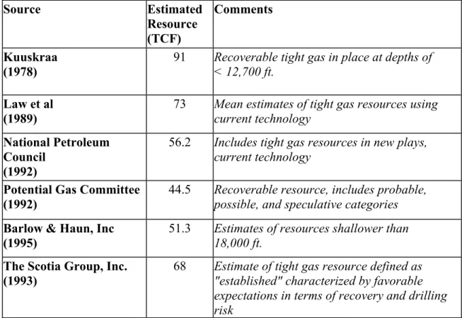
by several investigators (Table 2.1).
The Lewis Shale contains a significant underdeveloped gas resource. Although it
covers an area of 23,000 mi2 (59,146 km2), the Lewis Shale play has the fewest producing
wells in the Greater Green River basin (Figure 2.11). In terms of past production, as of
1996, the Lewis Shale had produced only 0.6 Tcf of gas or 6 percent of its 10.7 Tcf gas
resource. The Lewis Shale has 10.1 Tcf remaining gas supply (0.4 Tcf remaining reserves
and 9.7 Tcf undiscovered resource) (Table 2.2).
33 Source Estimated Resource (TCF) Comments Kuuskraa (1978)
91 Recoverable tight gas in place at depths of
< 12,700 ft. Law et al
(1989)
73 Mean estimates of tight gas resources using
current technology National Petroleum
Council (1992)
56.2 Includes tight gas resources in new plays,
current technology Potential Gas Committee
(1992)
44.5 Recoverable resource, includes probable,
possible, and speculative categories Barlow & Haun, Inc
(1995)
51.3 Estimates of resources shallower than
18,000 ft. The Scotia Group, Inc.
(1993)
68 Estimate of tight gas resource defined as
"established" characterized by favorable expectations in terms of recovery and drilling risk
Table 2.1. Various estimates of gas resources in the Greater Green River basin. (GRI, 1996).
Figure 2.11. The graph shows that the Lewis Shale play has the fewest producing wells in the Greater Green River basin. (GRI, 1996).
35
Table 2.2. As of 1996, the Lewis Shale produced only 0.6 Tcf
of gas, or 6 percent of its 10.7 Tcf gas resource.
Although the Lewis Shale has a large volume of remaining gas supply, there is a
low level of interest compared to other drilling objectives. Many reasons make the Lewis
Shale a difficult target for gas exploration and production. These reasons include
complex sandstone geometries, discontinuous sandstones, and poor reservoir quality.
Sandstone reservoirs in the basins have low porosity due to alteration by deep burial
cementation and other factors (Spencer, 1985). Gas-bearing sandstone reservoirs
associated with overpressure can also make the Lewis Shale a difficult target.
Most sandstone reservoirs of the Lewis Shale are located in the Red Desert Basin
and Wamsutter Arch area of the eastern Greater Green River basin (Doelger and Barlow,
1997). The setting for those production areas is a deep-water environment as submarine
fans with lobe-shaped geometry (Van Horn and Shannon, 1985; Winn et al., 1987;
Perman, 1987, 1990; Doelger and Barlow, 1997). These areas include a number of fields
such as Ten Mile Draw, Patrick Draw, Playa, Lost Creek, Great Divide, Wamsutter Arch,
Siberia Ridge, Echo Springs, Wild Rose, Standard Draw, Barrel Springs, Fillmore,
Creston, Table Rock, Stage Stop, Laney Wash, Emigrant Trail, Alkaline Creek, and Twin
Fork. Further south in the Washakie basin, the geometry of sandstone reservoirs becomes
more sheet-like. These reservoirs are associated with overpressure (Law et al., 1989). In
the south, fields include Polar Bar, Dripping Rock, Cepo, Triton, Smith Ranch, West Side
37
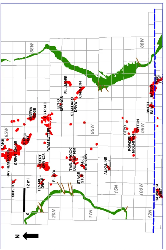
Figure 2.12. The map shows Lewis Shale production
in the Great Divide and Washakie basins.
12 mi
0
2.5 Petroleum System
A petroleum system encompasses a pod of active source rocks and all related oil
and gas and includes all of the essential elements and processes needed for oil and gas
accumulations to exist (Magoon and Dow, 1994). The presence of hydrocarbons is the
initial indication of a petroleum system. Four elements and two processes need to be
present in the correct order for a petroleum accumulation to occur. These four elements
are source rock, reservoir rock, seal rock, and overburden rock. Two processes of the
petroleum system, which are very important to be understood, are migration and trapping
mechanism. A better understanding of each element and each process can help to define
the petroleum system. Certain beds within the Lewis Shale contribute to the petroleum
system.
2.5.1 Source Rock
The first element of a petroleum system is the occurrence of source rocks. Source
rocks require both sufficient biological productivity to create large quantities of organic
matter and suitable depositional conditions for its concentration and preservation. Source
rocks are normally comprised of fine-grained sediment such as shale and shaly siltstone.
The best potential source rocks often occur in condensed sections where sedimentation is
restricted to pelagic and hemipelagic particles (Loutit et al., 1988). They are evaluated by
39
also evaluated by their hydrocarbon richness as atomic H/C or using Rock-Eval pyrolysis
as hydrogen index (HI).
In the study area, it has been suggested that carbonaceous shales in the lower part
of the Lewis Shale and thick coals of the Mesaverde Group provide excellent
hydrocarbon source rocks. Thick coals of the Mesaverde Group were suggested as the
source for gas in the overpressured zone in the Washakie basin (McPeek, 1981). The bed
in the lower part of the Lewis Shale was named the Asquith marker and was deposited
during sea level rise associated with the maximum transgression of the Lewis Seaway.
The Asquith marker is interpreted as the third-order condensed section deposited during
the Late Cretaceous (Pyles, 2000). It is comprised of black shale that is fissile,
organic-rich, and interbedded with bentonite beds. From several measurements of the Asquith
marker (Pyles, 2000), this bed contains TOC of 0.68% to 3.15%, which is sufficient for
hydrocarbon generation. From the Van Krevelen diagram, which is a hydrogen index and
oxygen index cross plot, the bed contains type II and III kerogens (Pyles, 2000).
2.5.2 Reservoir Rock
The second element of the petroleum system is reservoir rocks. Reservoir rocks
require both good porosity and good permeability. The quality of reservoir rocks is a
function of both porosity and permeability. Reservoir rocks are normally comprised of
medium to coarse-grained sediment such as sandy siltstone and sandstone. However,
associated with overpressure. Low porosity and low permeability in reservoir rocks may
be caused by deep burial cementation (Spencer, 1985).
The best potential reservoir rocks often occur associated with prograding
complexes where sedimentation occurs during a relative fall in sea level. The Dad
Sandstone member generally serves as the reservoir rock in the Lewis Shale. The Dad
Sandstone member is comprised of channel and sheet sandstones deposited during sea
level fall. The depositional system for these sandstones is interpreted to be submarine fan,
slope, and deltaic deposits.
2.5.3 Seal Rock
The third element of the petroleum system is the seal mechanism. While a
reservoir rock must be permeable, there must also be an impermeable seal above it that
prevents further upward migration of hydrocarbons. The seal element of the Lewis Shale
petroleum system is comprised of interbedded shales and bentonites. Zainal (2001)
observed the presence of good gas shows beneath bentonite markers in the Lewis Shale.
This suggests that bentonite markers have a good capability as a seal rock.
The sealing mechanism of the Lewis Shale petroleum system was likely a regional seal
deposited during a sea level rise.
Capillary pressure seals occur in the Washakie basin. Capillary pressure seals are
41
of two or more fluid phases in rock with very small pore throats reduces the effective
permeability (Meissner, 2000 and Law, 2002).
2.5.4 Overburden Rock
The fourth element of the petroleum system is the overburden rock. In the study
area, the Tertiary rocks act as overburden rocks. The deposition of the Tertiary rocks over
the Cretaceous and older source rocks can influence the maturation of source rocks. This
deposition can descend the source rocks into the hydrocarbon-generating window.
2.5.5 Hydrocarbon Generation, Expulsion, and Migration
Organic matter accumulated within sediment is buried in the basin by overlying
sediments. Organic matter then becomes subject to higher temperature and higher
pressure. Due to changes in temperature and pressure, the original composition of organic
matter is changed. The changes culminated in the production of liquid and gaseous
hydrocarbons. Thermal maturity of source rocks can be estimated by constructing cross
plots of Hydrogen Index (HI) and temperature maximum (Tmax) (Peters, 1986). Based
on the Van Krevelen diagram, which is hydrogen index and temperature maximum cross
plot, the Asquith marker samples are thermally mature. The temperatures ranged from
435 to 447 degrees Celsius. These values are close to the top of the oil window
Many of the features of petroleum generation in the source rock are understood, at
least in principle, but the timing and mechanism of migration are imperfectly known.
Because migration links the source rock to the reservoir rock, an understanding of the
migration mechanism is very important. The deeper burial through most of the Tertiary
can increase temperatures and pressures. With increased temperature, viscosity would
decrease, further allowing free movement of hydrocarbons.
The trap mechanism is also important in a petroleum system. Most traps that
occur in the Lewis Shale petroleum system are stratigraphic traps. Sandstone bodies that
pinch out against a paleohigh may create stratigraphic traps. Facies-change traps occur
when the sandstones were deposited within shale layers, or the sandstones had different
porosity compared to the surrounding sediments due to shale content. In addition,
structural traps also occur at Table Rock, Wamsutter, and Cherokee arch.
In fact, knowledge of the timing of certain geological events is the key to
evaluating petroleum prospecting (Jacobson, 1991). An event chart can help to evaluate
the petroleum system in order to define the critical moment. The critical moment is
defined as the selected point in time that represents the best situation for
generation-migration-accumulation of most hydrocarbons in the petroleum system. The event chart
shows the temporal relationship of the rock units, essential elements, processes,
preservation time and critical moment for this petroleum system in bar graph form (Table
43
Table 2.3. Event chart of the Lewis Shale petroleum syst
em in the Great Divide and Washakie basins, Wyoming.
CHAPTER 3
SUBSURFACE INTERPRETATION
3.1 Introduction
Stratigraphic correlation has been used by geoscientists to interpret subsurface
geology in Wyoming. For this study, the intent of using stratigraphic correlation is to
identify sandstone distributions and sandstone geometries.
This chapter discusses the regional subsurface geology of the Lewis Shale by
using a series of two-dimensional cross sections in the Great Divide and Washakie
basins. The discussion includes the distribution, geometry, and inferred paleocurrent
directions of sandstone lobes.
3.2 Previous work
In the study area, the Lewis Shale has been studied for several years by a number
of investigators for its stratigraphic complexity and significant gas and oil resources.
They studied many different aspects. They constructed cross sections across the Great
Divide and Washakie basins to better understand the depositional history of the Lewis
45
N
Lewis Shale outcrops Lewis Shale outcropsFigure 3.1. Map of the Red Desert and Washakie basins shows a series of cross sections constructed by Asquith (1970; IJ and KL cross sections), Weimer (1970; EF and GH cross sections), and Winn et al. (1985; AB and CD cross sections). After Winn et al. (1985).