Geometric Methods in the Study of the Snow Surface Roughness
Steven R. Fassnacht1ESS-Watershed Science, Colorado State University Iuliana Oprea, Patrick Shipman
Mathematics Department, Colorado State University James Kirkpatrick
Earth and Planetary Sciences, McGill University, Montreal George Borleske, Francis Motta
Mathematics, Colorado State University David Kamin
ESS-Watershed Science, Colorado State University
Abstract. The snow surface is very dynamic, and the roughness of the snowpack surface varies
spatially and temporally. The snow surface roughness influences the movement of air across the snow surface as well as the resulting transfers of energy, and is used to estimate the sensible and la-tent heat fluxes to and/or from the snow surface to the atmosphere. In the present work we used dif-ferent metrics, including the random roughness, autocorrelation, and fractal dimension, geometric roughness length, curvature, and power spectrum density to characterize the roughness of a typical snow surface. The data for the surface come from airborne LIDAR measurements taken during from the NASA Cold Land Process Experiment in late March 2003 at the Fraser Alpine intensive study area. The surface elevation data were rotated to be parallel to the dominant wind direction and were interpolated to a 1-m resolution. We provide a comparison of methods and present their possible applicability for other datasets.
1. Introduction
The snowpack is the interface between the atmosphere and the Earth. Snow surface roughness characteristics influence energy exchange, heat transfer, melting in the snow-pack, and thus are important input variables in snow-hydrologic models [Herzfeld et al., 2003]. Understanding the characteristics and the dynamics of the snow surface can im-prove our knowledge of hydrologic processes within the snowpack and their impact on melt dynamics and, further, on the climatology of the environment.
The surface of the snowpack changes over the winter. The surface roughness can in-crease or dein-crease during snow accumulation as the snow follows the underlying terrain in the initial stages of accumulation [Davison, 2004]. Alternatively, the snowpack surface can change due to redistribution with extreme features, such as sastrugi formed in wind-swept areas. The geometry of a snow surface can undergo dramatic temporal changes that influ-ence climate and hydrology, and how they are modeled. For example, Fassnacht [2010] showed that sublimation estimates using the bulk transfer formulae could vary by a factor of two by changing the aerodynamic roughness length (z0). This is a critical roughness
1 ESS-Watershed Science, Cooperative Institute for Research in the Atmosphere, and Geospatial Centroid, Colorado
State University, Fort Collins, Colorado, USA 80523-1476; phone: +001.970.491.5454; email: Steven.Fassnacht@colostate.edu
rameter whose prediction is of fundamental importance for estimating turbulent fluxes since this parameter enters in all existing numerical models of surface-atmosphere interac-tion. Therefore, accurate estimates of roughness are needed.
Various parameters and measures to describe surface-roughness from surface elevation data have been developed (see Dong et al., 1992, 1993, 1994 a,b; Smith 2014 for a re-view), and the proper choice depends on applications. Several metrics have been used to study the roughness of the snowpack surface from digital imagery [Fassnacht et al., 2009 a,b], but no comparison has been made between these metrics and the geometrically com-puted z0 of the snow.
In the present work we compare these metrics with the surface roughness length z0, on the same set of data. We use airborne light detection and ranging (LIDAR) estimates of the snow-pack surface elevation over a 200 by 200-m area. These elevations are at an approx-imate resolution of 1.3-m and have been interpolated to a 1-m resolution using ordinary kriging [Isaaks and Srivastava, 1989]. The purpose of this paper is to estimate i) the geo-metric-based z0 of a snowpack surface derived from an airborne LIDAR (light detection and ranging) dataset using the Lettau [1969] and Andreas [2011] methods, and ii) the roughness various other metrics (random roughness, auto-correlation, fractal dimension, scale break, power spectral density, curvature variation, and the direction of the principal maximum curvature) for the same set of surfaces (the entire area and the four 100 by 100-m blocks within it).
2. Methods
2.1. Roughness Length
The value of z0 is governed by roughness. A rough surface will enhance turbulence and increase atmospheric transfer rates over that surface, but reduce aeolian transport. Alt-hough z0 is a critical variable for estimating surface latent and sensible fluxes in numerical models, most land surface models treat z0 as a function of land cover type and usually as-sume it is constant over time for non-vegetated surfaces. For example, one of the more complex land surface schemes, the Community Land Model version 4.0 (CLM4.0), applies a single z0 value of 2.4 x 10⁻³ m to all snow-covered surfaces.
Yet, z0 has been reported to vary by orders of magnitude from 0.004 to 30 x 10-3 m for a variety of snow-covered glaciers [see Brock et al., 2006]. At any specific location, the physical roughness of the snow surface changes over the season [Fassnacht et al., 2009a]. The implication of variability in z0 was tested using a simple bulk transfer formulation for the latent mass flux; by altering z0 as a function of snow accumulation-settling or consider-ing directionality of the wind - sublimation estimates varied by at least a factor of two [Fassnacht, 2010].
The value of z0 was estimated from the measurement of surficial features [e.g., Lettau, 1969; Munro, 1989]. The dependence of z0 on the size, shape, density, and distribution of surface elements has been studied using wind tunnels, analytical investigations, numerical modeling, and field observations [Grimmond and Oke, 1999; Foken, 2008]. The lack of a clear formulation for calculating z0 as a function of surface roughness is due to the com-plexity of surface roughness that exists in nature. There are two approaches available to determine z0 for such surfaces: 1) micrometeorological or anemometric that relies on field observations of wind turbulence movement to solve for aerodynamic parameters included
or geometric that uses algorithms relating aerodynamic parameters to measures of surface morphometry [Grimmond and Oke, 1999; Foken, 2008]. In this study, geometric methods will be used with a spatially continuous database of the distribution of roughness elements surrounding the site of interest.
The most common geometric approach is simply a function of the height of the ele-ments:
z0 = f0 zH (1),
where zH is the mean height of roughness elements, and f0 is an empirical coefficient de-rived from observation.
The frontal area index (which combines mean height, breadth, and density of the roughness elements) is defined [Raupach, 1992] as roughness area density (λF) = Ly zH ρel, where Ly is the mean breadth of the roughness elements perpendicular to the wind direc-tion and ρel is the density or number (n) of roughness elements per unit area. Lettau (1969) developed a formula for z0 for irregular arrays of reasonably homogenous elements:
z0 = 0.5 zH λF (2).
Other methods have been developed, especially to consider more regularly-shaped and distributed roughness elements such as buildings in an urban setting [e.g., Counihan, 1971; Macdonald et al., 1998].
2.2 Autocorrelation-based Metrics
A variety of roughness metrics based on autocorrelation analyses have been developed to assess the roughness of a surface. Three common sets of roughness metrics are the random roughness (RR), auto-correlation (AC), and variogram analysis [Fassnacht et al., 2009b]. The RR is computed as the standard deviation of the detrended surface. In three-dimensions, a plane (or line in 2-D) is fitted to the dataset and used to remove trends that would otherwise bias the evaluation. These trends may be elevation gradients [e.g., Deems et al., 2006] or due to instrument/operator systematic biases [Fassnacht et al., 2009b]. The RR does not consider the spatial structure of roughness, except for the influence on detrending. However, evaluating how RR varies as a function of the length scale of the da-taset under consideration is a key measure of the fractal dimension of a system exhibiting scale-dependent roughness elements (e.g. Mandelbrot, 1983).The detrended data are used for the other two methods.
The AC does consider the spatial structure and requires that the detrended data be distributed on a regular interval. In 2-D it is the correlation coefficient of the each point along the curve with respect to the previous point, while in 3-D it is computed along each row and along each column to yield a series of X and Y AC values. In 2-D photographs of the snow surface are derived from the contrast with a black board inserted into the
snowpack [Fassnacht et al., 2009b]. A 3-D surface is often derived from (terrestrial or airborne) LIDAR that produces a cloud of points that must be interpolated to a regular grid (see Erxleben et al., 2002; López Moreno and Nogués Bravo, 2006 for a review of
An additional metric to test for periodic behavior in surface roughness is the power spectral density (PSD), which measures how the amplitudes, or heights, of the sinusoidal components of a 1-D profile vary as a function of frequency (or, equivalently,
wavelength). The PSD is calculated from a Fourier transform of an input profile that varies in height as a function of distance, assuming ergodicity of the system and that the profile is stationary (e.g. Percival and Walden, 1993). The transform results in a complex function in frequency that describes both the amplitude and phase of the input profile. The PSD
calculation re-quires a detrended, continuous, uniformly sampled dataset. Excursions in power at a par-ticular frequency or wavelength indicate periodic behavior in the signal. Systems that exhibit scale-dependent behavior are characterized by a power law
relationship between the PSD, P(λ), and length scale, λ, of the form P(λ)=Cλß, where C is a constant and ß is the average slope in log-log space. Self-similar profiles have ß=3, and self-affine profiles have ß<3. A break in slope in the PSD is often thought to correspond to a change in the physical process controlling the system. The influence of directional processes on the characteristics of a surface can be evaluated by taking cross-sections through a 3-D surface in particular directions with respect to the processes and calculating the PSD (e.g. parallel and perpen-dicular to the dominant wind direction for a snowpack).
Variogram analysis does not require a continuous dataset, or for the data to be on a regular interval, but still considers the spatial structure of the snowpack surface. Here the variance in elevation, i.e., surface height, among each pair of locations, i.e., points, in the data cloud is computed as a function of the distance between points. The semi-variogram (γ) is calculated as the average value of γ = ½(z(x)-z(x’))2 for all of the pairs of data points at a separation (lag) |x-x’|. The (semi-)variance is plotted as a function of the (lag) distance in log-log space and the fractal dimension (D) is computed as 3 minus the power of the best fit line divided by two [Deems et al., 2006]. This line is fitted up to the lag distance where the change in variance stops; this is scaled the scale break (SB). The variogram analysis can be performed with all data pairs, or can consider the direction of the pairs; Deems et al. [2006] used the main eight compass directions. Since the variogram is a type of autocorrelation function, the Fourier transform of γ results in the PSD.
2.3 Surface Curvature
A new curvature-based roughness metric, the curvature variation (CV) measures roughness as the total variation in the curvature of the surface. Specifically, the more that the curvature of the surface varies over space, the larger the value of this metric. A surface can be defined as a function, f(x,y), over a two-dimensional domain (x, y)∈Ω . The mean and Gaussian curvatures at a point, P(x,y) = (x,y,f(x,y)), on the surface are defined in terms of sectional curvatures considering the curves on the surface passing through P(x,y) formed by intersecting the surface with a plane perpendicular to the (x, y)-plane. Rotating that
plane, all such cross sectional curves are obtained, parameterized by the angle θ. Since the curvature of these curves is a continuous function of θ, there is an angle that yields a min-imum curvature, kmin, and an angle that yields a maximum curvature, kmax. The mean
cur-vature, H, at P(x,y) is:
H= 1
2(kmin+ kmax) (3),
K = kminkmax (4),
and is defined to be their product. The curvatures H and K are thus functions of (x, y)∈Ω . The curvature variation roughness metric is defined as the sum of the total var-iations of the mean and Gaussian varvar-iations over (x, y)∈Ω :
CV( f )= | ∇H |
(
2 + | ∇K |2)
dA Ω∫
(5).A larger value of CV for a surface indicates a rougher surface.
The angle yielding kmin and kmax always differ from each other by 90o or π/2 radians.
Therefore, one angle between ±π/2 radians determines the directions of both principle cur-vatures. The surface can also be characterized by the histogram of the distribution of direc-tions of maximum curvature over a uniform grid in (x, y)∈Ω . Since it goes between ±π/2 radians, it will be which will be reflected around the other half of the circle.
2.4 Dataset
Airborne lidar snow surface elevation data were collected in early April 2003 across the NASA Cold Land Process Experiment (CLPX) intensive study areas (ISAs) [Cline et al., 2009]. For this study, the Fraser Alpine (FA) ISA was used since the meteorological tower centered in the middle of the 1 km2 and much of this ISA was in an alpine area, i.e., not among trees. The meteorological data [Elder et al., 2009] were used to determine the dominant wind direction. All CLPX data were retrieved from the National Snow and Ice Data Center [Miller, 2004; Elder and Goodbody, 2004].
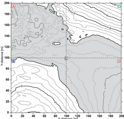
The raw surface elevation data were rotated to be with the direction of the dominant wind, and a 200 by 200m area (called block E) was extracted producing 28245 elevation points. The data were interpolated to a 1-m resolution using kriging in the SURFER soft-ware <http://www.goldensoftsoft-ware.com>. Holland et al. [2008] recommended interpolating LIDAR data to facilitate the computation of z0 from data on a regular grid. The area was divided into four sub-blocks (A, B, C, D) (see Figure 1). The analysis considered each 100-m block and the entire area (block E), as shown in Figure 1. Each of these five surfaces was detrended using a linear plane in X and Y.
3. Results and Discussion
Block A had the greatest roughness of the four blocks (Figure 1 and Table 1), and overall the combined block E was the roughest of all areas. This was illustrated from the RR and CV values, as well as the range of the data (Table 1). Other metrics highlighted other features of the data, but these may not be directly transferable to a bulk roughness value.
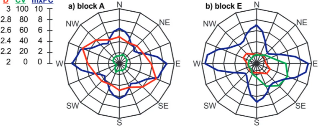
Some of the metrics are directional [Fassnacht et al., 2009b] and can be computed in X or Y (Table 1), while others can be computed radially (Figure 2). It should be noted that D, SB (where it was observed), and mxPC are in a direction across the entire block and thus symmetrical in a radial plot (e.g., Figure 2), while CV is from the center of the outward in a wedge.
The AC values approached unity or complete correlation, which is in part a function of the interpolation of the data. Since the autocorrelation is direction, it can be calculated for any row or column of data. In fact, the values presented here are an average. However, with the exception of block A and block B in the Y direction, all other AC values would
round to 1 with 2 significant figures. Subsequent analysis can examine individual rows or columns to highlight specific rougher strips; as well, the AC shown herein is for a lag of one meter and longer lags will show less autocorrelation. For example, for a lag of 10, AC ranged from 0.1 to 0.9 for different rows, i.e., along the X direction.
Figure 1. Contour map of the 200 by 200-m (block E) LIDAR-derived snow surface, illustrating the four sub-blocks (A, B, C, D). The surface has been detrended and the mean elevation is zero, thus the areas below the mean are shown in grey. The meteorological tower is located in the middle of block A. The power spectral density (Figure 3) can present similar results to the variogram-based D, but the former does require regularly spaced data, i.e., interpolated data. It pre-sents the roughness characteristics illustrated by RR for the different blocks.
There can be an order of magnitude difference in the geometric z0 due in part to the limitations of the Lettau [1969] method. The Lettau method “works well when roughness elements are fairly isolated” [Businger, 1975]. When the cross-sectional area of a rough-ness element becomes similar to the horizontal area of the element, z0 tends to be overes-timated.
Recent advances in surveying have improved the resolution, extent and availability of topographic datasets, allowing geometric characterizations. This paper outlines methods directed towards the new ways of collecting data from various means, including satellite, airborne and terrestrial LIDAR [Deems et al., 2013] and photogrammetry [Fabris and Pesci, 2005].
Table 1. Summary of the snow surface data, roughness lengths (z0) from Lettau and Andreas, and rough-ness metrics (RR = random roughrough-ness, AC = autocorrelation, D = fractal dimension, SB = scale break, CV = curvature variation, mxPC = % of histogram with that maximum principal curva-ture) for the different blocks. Notes: N/A = not applicable, i.e., a value does not exist, and n/c = not computed. block A B C D E maximum of data 2.64 1.10 1.91 1.84 6.66 minimum of data -2.12 -1.78 -1.23 -1.31 -4.90 RR 0.738 0.428 0.572 0.492 1.95 AC in X 0.980 0.995 0.996 0.994 0.998 AC in Y 0.988 0.984 0.996 0.998 0.999 omni-directional D 2.23 2.28 2.24 2.17 2.18
omni-directional SB [m] 5.25 40 48 N/A N/A
Lettau z0 in [x10-3m] 4.81 146 59.4 10.8 52.8 Lettau z0 in [x10-3m] 2.10 139 35.7 0.76 25.5 Andreas z0 in X [x10-3m] n/c n/c n/c n/c 0.92 Andreas z0 in Y [x10-3m] n/c n/c n/c n/c 0.95 D along X (short) 2.58 n/c n/c n/c 2.17 D along Y (short) 2.49 n/c n/c n/c 2.17
CV along X from upwind 8.59 4.24 3.81 3.64 15.2
CV along Y from upwind 13.9 3.49 5.95 3.49 16.4
mxPC (% in X direction) 8.62 11.9 10.2 7.98 9.39
mxPC (% in Y direction) 6.39 8.15 6.44 7.59 6.98
CV along X downwind 12.3 3.73 6.30 3.46 53.3
CV along Y downwind 12.1 4.96 9.45 3.60 25.2
Figure 2. Radial plots for a) block A and b) block E showing the directionality of the fractal dimen-sion (D is between 2 and 3), the curvature variation (CV is between 0 and 100), and the distribution of the maximum principal curvature (maxPC is between 0 and 10%). All metrics are unitless.
4. Summary
Snow surface roughness varies over space, and while not shown here, it does vary over time [e.g., Fassnacht et al., 2009]. The different metrics yield varying results, as discussed by Smith [2014]. Further analyses need to examine how the different metrics can be merged to yield composite values. Often the aerodynamic z0 value is desired for modeling; if this can be more adequately estimated from geometric methods, it can be better scaled and more accurately used in hydrological, climate, and other models.
Acknowledgements. Partial support was provided by the National Science Foundation
through a Colorado State University (CSU) Center for Interdisciplinary Mathematics and Statistics (CIMS) grant, as well as a grant from the Colorado Water Center at CSU.
Figure 3. Power spectral density (PSD) as a function of wavelength for the four sub-blocks (A,B,C,D) and the entire block (E). The solid lines are west to east and the dashed lines are north to south.
References
Andreas, E.L, 2011: A relationship between the aerodynamic and physical roughness of winter sea ice.
Quar-terly Journal of the Royal Meteorological Society, 137, 1581-1588.
Brock, B.W., I.C. Willis, and M.J. Sharp, 2006: Measurement and parameterization of aerodynamic rough-ness length variations at Haut Glacier d’Arolla, Switzerland. Journal of Glaciology, 52(177), 281-298. Businger, J.A., 1975: Aerodynamics of vegetated surfaces. In Heat and Mass Transfer in the Biosphere: Part
1. Heat Transfer in the Plant Environment, (eds. D.A. de Vries and N.H. Afgan), pp. 139– 165, Scripta
Book Co., Washington, D.C.
Cline, D., S. Yueh, B. Chapman, B. Stankov, A. Gasiewski, D. Masters, K. Elder, R. Kelly, T.H. Painter, S. Miller, S. Katzberg, and L. Mahrt, 2009: NASA Cold Land Processes Experiment (CLPX 2002/03): Airborne Remote Sensing. Journal of Hydrometeorology, 10(1), 338-346.
Counihan, J., 1971: Wind Tunnel Determination of the Roughness Length as a Function of the Fetch and Roughness Density of Three Dimensional Roughness Elements. Atmospheric Environment, 5, 637-642. Davison, B.J., 2004: Snow Accumulation in a distributed Hydrological Model. Unpublished M.A.Sc. thesis,
Civil Engineering, University of Waterloo, Canada, 108pp + appendices.
Deems, J.S., S.R. Fassnacht, and K.J. Elder, 2006: Fractal distribution of snow depth from LiDAR data.
Journal of Hydrometeorology, 7(2), 285-297, [doi:10.1175/JHM487.1].
100 101 102 10−6 10−5 10−4 10−3 10−2 10−1 100 101 Wavelength (m) PSD (m 3)
PSD Comparison: dashed lines are N−S, solid E−W
DKR
AKR
EKR
CKR BKR
Dong, W.P., P.J. Sullivan, and K.J. Stout, 1992: Comprehensive study of parameters for characterising three-dimensional surface topography I: Some inherent properties of parameter variation. Wear, 159(2), 161-171.
Dong, W.P., P.J. Sullivan, and K.J. Stout, 1993: Comprehensive study of parameters for characterising three-dimensional surface topography II: Statistical properties of parameter variation. Wear, 167(1), 9-21. Dong, W.P., P.J. Sullivan, and K.J. Stout, 1994a: Comprehensive study of parameters for characterising
three-dimensional surface topography: III: Parameters for characterising amplitude and some functional properties. Wear, 178(1-2), 29-43.
Dong, W.P., P.J. Sullivan, and K.J. Stout, 1994b: Comprehensive study of parameters for characterising three-dimensional surface topography: IV: Parameters for characterising spatial and hybrid properties.
Wear, 178(1-2), 43-60.
Delaunay, B., 1934: Sur la sphère vide. Izvestia Akademii Nauk SSSR, Otdelenie Matematicheskikh i
Estestvennykh Nauk, 7, 793-800.
Elder, K. and A. Goodbody, 2004: CLPX-Ground: ISA Main Meteorological Data - Fraser Alpine ISA. NASA DAAC at the National Snow and Ice Data Center, Boulder, Colorado USA.
Elder, K., J. Dozier, and J. Michaelsen, 1991: Snow accumulation and distribution in an alpine watershed.
Water Resources Research, 27(7), 1541-1552.
Elder, K., D. Cline, A. Goodbody, P. Houser, G.E. Liston, L. Mahrt, and N. Rutter, 2009: NASA Cold Land Processes Experiment (CLPX 2002/03): Ground-Based and Near-Surface Meteorological Observations.
Journal of Hydrometeorology, 10(1), 330-337.
Erxleben, J., K. Elder, and R. Davis, 2002: Comparison of spatial interpolation methods for estimating snow distribution in the Colorado Rocky Mountains. Hydrological Processes, 16(18), 3627–364.
Fabris, M., and A. Pesci, 2005: Automated DEM extraction in digital aerial photogrammetry: precisions and validation for mass movement monitoring. Annals of Geophysics, 48(6), 973-988.
Fassnacht, S.R., 2010: Temporal changes in small scale snowpack surface roughness length for sublimation estimates in hydrological modeling. Journal of Geographical Research, 36(1), 43-57.
Fassnacht, S.R., M.W. Williams, and M.V. Corrao, 2009a: Changes in the surface roughness of snow from millimetre to metre scales. Ecological Complexity, 6(3), 221-229.
Fassnacht, S.R., J.D. Stednick, J.S. Deems, and M.V. Corrao, 2009b: Metrics for assessing snow surface roughness from digital imagery. Water Resources Research, 45, W00D31.
Foken, T., 2008: Micrometeorology. Springer Verlag.
Grimmond, C.S.B., and T.R. Oke, 1999: Aerodynamic properties of urban areas derived from analysis of sur-face form. Journal of Applied Meteorology, 38, 1262-1292.
Herzfeld,U.C, M. Helmut, N. Caine, M. Losleben, and T. Erbrecht, 2003: Morphogenesis of typical winter and summer snow surface patterns in a continental alpine environment. Hydrological Processes, 17, 619-649
Holland, D.E., J.A. Berglund, J.P. Spruce, and R.D. McKellip, 2008: Derivation of effective aerodynamic surface roughness in urban areas from airborne lidar terrain data. Journal of Applied Meteorology and
Climatology, 47, 2614-2625.
Isaaks, E.H., and R.M. Srivastava, 1989: An Introduction to Applied Geostatistics. Oxford University Press, New York.
Lettau, H., 1969: Note on Aerodynamic Parameter Estimation on the Basis of Roughness-Element Description. Journal of Applied Meteorology, 8, 828-832.
López Moreno, J.I. and D. Nogués Bravo, 2006: Interpolating snow depth data: a comparison of methods.
Hydrological Processes, 20(10), 2217-232 [doi:10.1002/hyp.6199].
Macdonald, R.W., R.F. Griffiths and D.J. Hall, 1998: An improved method for the estimation of surface roughness of obstacle arrays. Atmospheric Environment, 32, 1857-1864.
Mandelbrot, B.B., 1983: The Fractal Geometry of Nature. Freeman, New York.
Manninen, T., K. Antilla, T. Karjalainen and P. Lahtinen, 2012: Instruments and Methods - Automatic snow surface roughness estimation using digital photos. Journal of Glaciology, 58, 211, [doi:
10.3189/2012JoG11J144]
Miller, S. 2004: CLPX-Airborne: Infrared Orthophotography and Lidar Topographic Mapping - Fraser
Al-pine ISA. NASA DAAC at the National Snow and Ice Data Center, Boulder, Colorado USA.
Munro, D.S., 1989: Surface roughness and bulk heat transfer on a glacier: Comparison with eddy correlation.
Percival, D.B., and A.T. Walden, 1993: Spectral Analysis for Physical Applications. Cambridge University Press.
Raupach, M. R., Drag and drag partition on rough surfaces, Boundary Layer Meteorol., 60, 375–395, 1992. Smith, M.W., 2014: Roughness in the Earth Sciences. Earth-Science Reviews, 136, 202-225.