SKI Report 99:11
Spatial Variability of Geosphere
Parameters and the Impact of the
F-ratio on Radionuclide Release
ISSN 1104-1374
António Pereira
SKI Report 99:11
Spatial Variability of Geosphere
Parameters and the Impact of the
F-ratio on Radionuclide Release
António Pereira
Dept. of Physics, Stockholm University,
Box 6730, SE-113 85 Stockholm, Sweden
March 1999
This report concerns a study which has been conducted for the Swedish Nuclear Power Inspectorate (SKI). The conclusions and viewpoints presented in the report are those of the author and do not
SKI Project Number 98006
Abstract
The interpretation of the F-number as a transport resistance to groundwater flow and to radionuclide transport is investigated for a 1D model representation of heterogeneous fractured rock divided into blocks with definable averaged value parameters
characterising those blocks.
It is concluded that the physical interpretation of the F-number as a resistance in 1D advection-dispersion transport models can be generalised under certain conditions to models that can cope with the intrinsic variability of flow parameters along the transport pathway, an example of these models being the multiple-leg models. The constraints imposed upon these conditions is that both the F-ratio and the longitudinal dispersion are additive. Outside of this domain of validity, the F-number looses its physical significance as a resistance of the rock to groundwater flow and also to radionuclide transport. This is shown by the calculations using decaying species or when the chemistry also varies along the transport pathway.
In summary, in 1D multiple-leg transport models, the F-number is a transport resistance offered by the rock to the groundwater flow, but it does not represent a resistance to radionuclide transport. The F-number allows one to make use of site characterisation data to reduce the range of uncertainties in the flow parameters extracted from field data and hydrogeological calculations in the performance assessment.
It is also concluded that it is necessary to develop a new class of transport models that explicitly take into account the intrinsic spatial variability of rock properties.
Investigation of the impact of spatial variability of parameters on the consequences delivered by this class of transport models is therefore an important task in relation to uncertainty and sensitivity analyses of the performance assessment of geological repositories.
Abstract (Swedish)
Tolkningen av F-talet som ett transportmotstånd mot grundvattenflödet (Darcy-flödet) och också mot radionuklidtransport, har undersökts för endimensionella modeller av nuklidtransport i geologiskt heterogen och sprucken berggrund. Konceptuellt består berggrunden av enskilda block som karaktäriseras av vissa parametrar med definierade medelvärden.
Vi visar att den fysikaliska tolkningen av F-talet som ett transportmotstånd för
endimensionella transportmodeller av advektion-dispersions typ kan generaliseras under vissa villkor till transportmodeller som tar hänsyn till den naturliga variabiliteten av flödesparametrarna längs radionuklidernas transportsträckor som t.ex. modeller med flera transportsträckor kopplade i serier. De ovannämnda villkoren är att både F-talet och den longitudinella dispersionen är additiva parametrar. Utanför denna
validitetsdomän förlorar F-talet dess betydelse som ett kvantitativt definierbart mått på berggrundens motstånd gentemot Darcy-flödet.
De ovannämnda slutsatserna dras med hjälp av numeriska experiment där man har simulerat transporten av kontaminanter som inte sönderfaller och också av radionuklider både med och utan hänsyn till rumsvariabilitet av flödes-och transport parametrar längs transportsträckorna.
Sammanfattningsvis gäller det att F-talet är, för endimensionella modeller, ett
kvantitativt mått på det motstånd mot Darcy-flödet som berget utgör, men att det inte lämpar sig som ett moståndsmått för radionuklidtransport.
Flödesparametrar som härleds från fältdata och hydrogeologiska beräkningar från en platsundersökning är alltid behäftade med osäkerheter. Den fysikaliska tolkningen av F-talet som ett motstånd mot Darcy-flödet gör det principiellt möjligt att reducera effekten av dessa osäkerheter i utvärderingar av potentiella förvaringsplatser och därtill kopplade säkerhets- och känslighetsanalyser.
Det står också klart att det är nödvändigt att utveckla en ny typ av transportmodeller som på ett explicit sätt kan ta hänsyn till den naturliga variabiliteten hos de fysiska och kemiska egenskaperna hos berggrunden längs nuklidernas transportsträckor.
Den påverkan av parametrarnas rumsvariabilitet på konsekvenserna som fås som resultat av simuleringar med denna typ av transportmodeller är därför av stor betydelse inom säkerhets-och känslighetsanalyser i utvärderingen av ett djupförvar.
Contents
1 Introduction 1
2 A conceptual approach to transport modelling in heterogeneous
fractured media 3
2.1 Introduction 3
2.2 Flow parameters and the role of the F-ratio 4
3 The computational approach 7
3.1 Introduction 7
3.2 Specification of case studies 7
4 The impact of the F-ratio on radionuclide release for spatially varying
flow parameters 11
4.1 The double-leg model: Results and discussion 11
4.1.1 Variation of the flow-wetted surface area and longitudinal dispersion
for constant Peclet numbers −− Cases A0 and A1 11
4.1.2 The impact of the F-ratio with the Peclet numbers varying along the
path −− Case A2 16
4.2 The ten-leg model: Results and discussion 17
4.2.1 Stable species − Case B1 17
4.2.2 Decaying species − Case B2 19
5 The impact of the F-ratio on radionuclide release for simultaneous
variations in the flow and transport parameters 23
5.1 Introduction 23
5.2 The fully coupled transport model −− Case B3 23
6 Summary and conclusions 26
References 29
Appendix I 31
1. Introduction
In fractured heterogeneous media like granite, radionuclide migration is dominated by advective solute transport in groundwater circulating in the fracture system. In this system, surface sorption and matrix diffusion are two phenomena that play an important role in the retardation of the nuclides. The impact of surface sorption and matrix
diffusion is partially limited by the fractures’ flow-wetted surface area, as this area defines the total surface available for sorption (reversible or irreversible). It is also through this area that nuclides can migrate into the rock matrix by diffusion. Within the pore water of the matrix the nuclides are trapped for longer or shorter times and are therefore not directly available for advective transport by water in the fractures.
The migration of radionuclides in the network of fractures is usually estimated with the help of 1D advection-dispersion models (AD models), which are also able to treat radioactive decay chains and interactions between the nuclides and the surrounding environment. A representative code of this class of AD transport models is CRYSTAL (Robinson and Worgan, 1992), which has been extensively used in SKI’s Project-90 (1991) and SITE-94 (1996). The input parameters used in CRYSTAL come in part from field data and in part as soft data extracted from hydrogeological modelling of groundwater flow in fractured media. The CRYSTAL model requires two types of input parameters: flow and transport parameters. Flow parameters are related to the movement of the groundwater in the system of fractures and can be subdivided into two groups of equivalent parameters given by two numbers: the F-ratio and the Peclet number. The F-ratio represents a measure of the capacity for retardation in the rock, i.e., a resistance the rock offers to groundwater flow. The Peclet number is the ratio between advective to dispersive groundwater transport. The transport parameters contain information related to the physical processes and the chemical interactions between the nuclides and the host rock. An important transport parameter in CRYSTAL is given by a lumped parameter, the distribution coefficient.
One disadvantage of the transport codes commonly used nowadays is that they cannot handle the impact of the spatial variability of flow and transport parameters, arising from rock heterogeneity. There are two possible ways of solving this problem. The first one is, as in our case, to extend the CRYSTAL code to include such a capability. The second one is to develop a new transport code for heterogeneous media. With these two alternatives in mind, the aim of this report is two-fold:
• To investigate the impact of the F-ratio on the prediction of consequences of
radionuclide migration when the spatial variability of flow parameters is taken into account and compare it to situations in which variability is ignored.
• To extend the above investigation by including the spatial variability of transport
parameters, in our case the spatial variability of the distribution coefficient.
To address those two aims we use a model with multiple legs here, which is based on the CRYSTAL model.
The first aim is the main target of this work. It is related to how and to what extend we can use information from site characterisation (as in, for instance, how averaging of data
is done in the reduction of 3-D data to a one-dimensional form) in transport models to reduce the uncertainty introduced by different sources.
The second aim is of relevance if one is to examine the capabilities needed by a new transport model. Do we need a more flexible way of treating spatial variability of parameters than the one that a multiple-leg CRYSTAL model can offer? And if so,
why?1
For a multiple-leg model we need to give a precise definition of how the F-ratio should be interpreted. Therefore the definition of the F-ratio as a resistance will be used in the sequel in the sense that physical resistances are additive. If in a multiple-leg model the impact resulting from summing several partial F-ratios is the same as the impact resulting from the F-ratio of the corresponding single-leg model, we will say in such a case that the F-ratio is a resistance. In the opposite situation the F-ratio concept does not work as a resistance.
In Section Two we introduce a background to the heterogeneity of fractured media and consider its implications for the modelling of radionuclide transport. In this section we motivate the suggested conceptual approach. In Section Three, the computational approach used to address the above mentioned questions is presented together with the choice of case studies and input data common to all calculations. The results are presented and discussed in Section Four for the flow problem (impact of F-ratio on radionuclide release in the presence of variability of flow parameters) and in Section Five they are presented and discussed for the fully coupled transport problem (that is, the impact of the F-ratio on radionuclide release is examined for the case of
simultaneous variability of the flow and transport parameters). The summary and the conclusions are presented in Section Six, which is followed by references and
appendixes.
1
Another aspect of those capabilities is the easy of handling time-dependent parameters, which is not addressed in this report.
2. A conceptual approach to transport modelling in
heterogeneous fractured media
2.1 Introduction
Strong evidence exists (Neretnieks et al., 1987) that solute transport in fractured media is dominated by channelling. The solutes move in a 3 dimensional network of fractures with variable apertures, lengths and orientation in space. Some of those fractures can be highly conductive (channels) in which the transport is dominated by advection, whereas in others groundwater can flow only with difficulty. In the 1D model conceptualisation, this network is represented by an equivalent fracture or system of plane parallel
fractures, a model that is an extension of well working and very useful models for porous media. In these 1D model formulations like CRYSTAL, the migration
Figure 1 Schematic representation of heterogeneous fractured media for three different
blocks characterised by groups of fractures with similar properties.
path is represented by a single transport length L, representing an effective mean
transport length.
CRYSTAL´s analytical solution does not allow one to examine the implicit variability of parameters and the heterogeneity along the transport pathway. One possible approach by which to introduce these effects is to consider a conceptual model in which we assume that the rock is divided into blocks, each representing a class with more or less definable characteristics, such as the intensity and orientation of the fractures, the net connectivity, the total flow-wetted surface area, etc, (Fig.1). Assume also that for each class (block), it is possible to extract average values for the flow parameters. In this representation each class i is a block with a given length Li . Assume also that the
transport length L for the entire migration path in the rock is divided into several
1 2 3 Repository well Heterogeneous fractured media
segments L1 , L2 etc., one for each block, such that their sum is equal to L. Now, it will
be possible to vary the flow and transport parameters along the transport pathway by
using CRYSTAL to model each segment Li separately, where each segment is
characterised by its own parameters. Because the segments are connected in series, the
output from one simulation using CRYSTAL, say for the segment Lj , is used as source
term for the next simulation L j+1.
2.2 Flow parameters and the role of the F-ratio
Every single rock fracture is geometrically characterised by its length, aperture and width. Due to channelling only a fraction of the fracture surface is wetted (fig.2).
Figure 2 Schematic representation of a fracture with its flow-wetted surface area.
The flow-wetted surface area enters as an input parameter in certain models for migration in fractured media. In the CRYSTAL model (Robinson and Worgan, 1992) the flow-wetted surface area is related to the volume of rock. This parameter is a multiplicative factor in the so-called F-ratio:
where, F [s/m] is the F-ratio , a [m2/m3] is the flow-wetted surface area per volume of
rock, L [m] is the migration path length and q [m/s] is the Darcy velocity. Physically, F
represents a measure of geosphere resistance to groundwater flow. The spatial
variability of the flow-wetted surface along the transport path of radionuclides makes F
a spatially dependent entity.
Now, assuming that the Darcy flow, q, and the flow-wetted surface area, a, or their ratio
are kept constant along the transport pathway, it follows from Eqn. 1 that the F-ratio F
for the total pathway L will be equal to the sum of Fi´s , the F-ratio of each segment i:
For the conceptual model discussed above, does Eqn.2 imply that the F-ratio for the
total path length L is still a representative number for the transport resistance of the rock
to groundwater flow? If it is, the radionuclide releases obtained by our transport model
Flow-wetted surface area
∑ = i iF F (2) F =aL q ( )1 Fracture plane
should be quite insensitive to variations of q, a and L as long as their relationship is
such that the F-ratio has the same value. In such case, the additivity of the F-ratio
implies that it should be possible through site characterisation, to extract the partial F-ratios Fi, for each region, and use the sum as an effective F-ratio for the rock as a
whole, instead of using them in transport models that can cope with spatial variability. As pointed out before this is the first question addressed by this work. To confirm or reject this possibility we assume here that:
• The longitudinal dispersion is proportional to the transport length in each block i.e.
the Peclet number is the same for all blocks.
• The transport parameters are also the same for all blocks i.e. there is no variability
along the pathway for these parameters within each block.
The second question is the usefulness of the F-ratio parameter in transport models for heterogeneous media, when we allow all parameters and not only the flow parameters to vary spatially. Again we assume that the F-ratio is still such that it is equal to the sum of the F-ratios of the segments, and that the Peclet number is constant in accordance with our conceptual model. But we do not put other restrictions on the variations on the transport parameters along the transport pathway, i.e., flow and transport parameters are allowed to vary simultaneously. In one case study (see Section 4.1.2), there will be a deviation from the assumption of a constant Peclet number for reasons to be discussed later.
3. The Computational approach
3.1 Introduction
To allow variability in the parameters along the transport pathway, i.e. to introduce variability in some of the properties from fracture to fracture (or block to block), we segment the transport length L into a certain number of shorter distances L1, L2, etc.,
each of which represents a new fracture or groups of fractures with the same
characteristics. The CRYSTAL model was then used to construct a multiple-leg model, which allows one to simulate the transport in this set of fractures, which is viewed as being connected in series. This approach has been used for Monte Carlo simulations (Andersson et al., 1997), (Pereira et al., 1997) to introduced parameter variability along the transport pathway in probabilistic calculations of radionuclide transport.
In this report the same idea of segmentation is used to address the interpretation and the impact of the F-ratio on model predictions. In a first set of case studies comprising
cases A0, A1 and A2, the transport length L is divided in two segments (double-leg case)
for a certain set of input parameters that correspond to variations of some of the deterministic far-field case studies in SITE-94 (1996). This study is generalised in the
second set of case studies, cases B0 - B3, in which the transport length L is divided into
ten legs. The results of the simulations obtained by segmentation are then compared
with those of simulations with a single path length L. For all cases the sum of the
F-ratios corresponding to each segment is equal to the F-ratio for the non-segmented (single-leg) path. This procedure allows us to draw conclusions about the role and impact of the F-ratio as a measure of the resistance of the rock to groundwater flow and to radionuclide transport.
3.2 Specification of case studies
For the sake of completeness the system of partial differential equations used in the CRYSTAL model is given bellow,
1 n 1 n 1 n n n n 0 m n m m 2 n 2 n n n R C R C C D a x C D x C u t C R − − − = + − + + − = λ λ ω ∂ ∂ θ θ ∂ ∂ ∂ ∂ ∂ ∂ ω (3a) R C t D C R C R C nm n m m nm nm n nm nm n nm ∂ ∂ ∂ ∂ ω λ λ = 2 2 − + −1 −1 −1 (3b)
where, Rn is the retardation attributable to sorption on the fracture walls and Rnm the
retardation due to the matrix; these retardation coefficients are given respectively by
θ δ θ ρ K (1 )a / 1 R m n , d m n = + − and m m m n , d m n 1 K (1 )/ R = + ρ −θ θ . The subscript n
denotes the nth radionuclide in the chain. Cn(x,t) [moles/m3] is the concentration of
radionuclides in the fracture water, t [years] the time, u [m/year] the velocity of water in
the fracture, x [m] the distance along the pathway, D [m2/year] the longitudinal
porosity, a [m-1] the specific flow-wetted area per volume of the rock mass, δ [m] the
”depth” of surface sorption, Kd,n [m3/kg] the distribution coefficient, Cnm(x,ω t,)
[moles/m3] the concentration of radionuclides in the rock matrix pore water, ω [m] the
distance perpendicular to the fracture, δ [m] the maximum penetration depth in the ω
direction and λ [(year)-1] the radioactive decay constant.
In the choice of the case variations, the following should be kept in mind:
• The F-ratio for the simulation of the total path length L is equal to the sum of
F-ratios for the different blocks (see equation 2).
• The Peclet number is constant along the transport pathway, (i.e. the longitudinal
dispersion must be proportional to the transport pathway length), unless otherwise stipulated.
• The impact of the F-ratio on the outcomes obtained by CRYSTAL as addressed by
the first aim of this work, is studied for constant transport parameters and only for the double-leg model.
• The impact of the F-ratio on the consequences for the general case i.e. for the
simultaneous variation of flow and transport parameters is only analysed using the ten-leg model.
There is one situation where the Peclet number is allowed to vary along the transport pathway. The motivation for this will be given later when the outcome is discussed. Regarding the near-field data necessary for the simulations, the only requirement is that the same source term must be used in all simulations if one is to be able to compare the
results. We have used a pulse of constant amplitude (equal to 106 Bq/year) and with a
duration of 7.4x10⁴ years in all calculations.
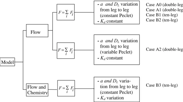
Fig. 3 shows a diagram of the cases considered and how they are calculated.
Figure 3 Scheme showing the choice of case studies for the double-leg and the ten-leg
models. Case B3 (ten-leg) Case A2 (double-leg) Case A0 (double-leg) Case A1 (double-leg) Case B1 (ten-leg) Case B2 (ten-leg) - a and DL tion from leg to leg (constant Peclet)
- Kd variation
- a and DL variation from leg to leg (variable Peclet)
- Kd constant
- a and DL variation from leg to leg (constant Peclet) - Kd constant Flow Model Flow and Chemistry ∑ = i iF F ∑ = i iF F ∑ = i iF F
Table I shows a summary of the cases considered in the calculations. The parameters that are not varied are taken from SITE-94 calculation cases. Some of the far-field parameters used by the CRYSTAL model are always kept constant, see Table II.
Table I Summary of case studies. Case No. of
Legs Radioactive decay Variationin a Variationin DL
Variation
in Pe Variationin Kd
A0 2 Stable species Yes Yes No No
A1 2 Stable species Yes Yes No No
A2 2 Stable species Yes Yes Yes No
B1 10 Stable species Yes Yes No No
B2 10 Decaying species Yes Yes No No
B3 10 Decaying species Yes Yes No Yes
Tables 2, 3 and 4 in Appendix I, present the input data for the “double-leg” model (cases
A0, A1 and A2 respectively) and Table 5the input data for the “ten-leg” model (cases
B1, B2, and B3). For the convenience of the reader these tables not only present the parameters that vary from case to case, but also the constants shown in Table II.
Table II Far-field parameters common to all case variations.
Parameter Value Unit
Fracture spacing, S 1.0 m
Penetration depth, Pdepth a) 5.0x10⁻² , b)5.0x10⁻¹ m
Rock matrix porosity, gp 1.0x10⁻³
-Diffusion coefficient in the pore
water of the rock matrix, Dm 9.5x10⁻⁴ m2/year
Sorption coefficient, Kd 0†, 1.0 m3/kg
a) Cases A0-A2. b) Cases B1-B3.
† Only cases A0 and B2 have a zero distribution coefficient.
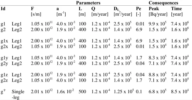
We illustrate the way the tables of input data should be read by taking Table 3 in
Appendix I as the starting point. Consider the case shown by the rows a1x, a2x and a3.
Row a3 gives the parameters corresponding to the single-leg case (with path length L)
to be simulated by CRYSTAL. Rows a1x and a2x give the input parameters for the first
a2x together represent one simulation. First the radionuclide transport through L1 is
simulated using the rectangular pulse of amplitude 106 Bq/years and a duration of
7.4x10⁴ years as the source term and the result of this first simulation is then used as the
source term for the transport through the second pathway L2. In the analysis the result
obtained at the end of L2 , row a2, should, therefore, be compared with the one obtained
from row a3 (for L = L1 + L2 and for “single-leg” respectively).
Rows a1y and a2y define a new simulation, which is also to be compared with a3. The
pairs (a1x,a2x) and (a1y,a2y) represent two variations that to be compared with a3, a3
being the case whose F-ratio number is equal to the sum of the F-ratio of the pairs. In
the same way all rows starting with b in the same table, i.e. (b1x, b2x) and (b1y, b2y)
should be compared with b3.
All cases are based upon data from Table 15.2.12 of the SITE-94 report (1996). The comment lines in the tables of the appendixes give the case labels used in the SITE-94 report.
4. The impact of the F-ratio on radionuclide release
for spatially varying flow parameters
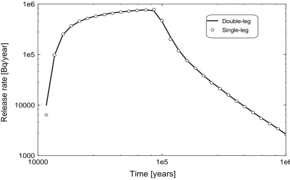
A test case was defined in which the path length L is divided into two equal segments in
length L1 and L2 . The input parameters (see Appendix I, Table 1) are also equal for
these two path lengths and therefore the outcomes of the simulation of the single migration path and of the segmented path with two legs, should be the same. Figure 4 below shows the results. There is a good agreement between calculations for the single and the double-leg cases.
Figure 4 The breakthrough curves for the simulations of a single path (single-leg
model) and the segmented path (double-leg model), result in equivalent breakthrough curves.
In subsequent sections the results are presented in the following order: firstly, the double-leg calculations, and secondly the ten-leg calculations. The outcomes to be compared are: a) the peak releases and the time at which they occur and b) the overall shape of the release rate curves as a function of time.
4.1 The double-leg model: Results and discussion
4.1.1 Variation of the flow-wetted surface area and longitudinal dispersion for constant Peclet numbers −− Cases A0 and A1.
These double-leg calculations correspond to cases A0 and A1. The input data for the
two cases differ in the Kd parameters, which are zero for case A0 and 1.0 m3/kg for case
A1. The half-life is set to infinity, i.e., we simulate non-decaying species. The results of
Time [years]
Release rate [Bq/year]
1000 10000 1e5 1e6 10000 1e5 1e6 Double-leg Single-leg
the simulations are summarised in Table III (case A0 ) and IV (case A1). These tables
also include the results of the calculations with a non-segmented path length L, which
are labelled “single leg”. The two columns on the right show the peak releases and the time at which they occur.
Tables III and IV show that the differences between the peak releases for the single and double-leg simulations are small. In all cases changing the position of leg 1 with that of leg 2, i.e., taking for example the simulations of the two legs in the order (s1x, s2x) instead of the reversed (s2x,s1x) (which corresponds to (s1y, s2y) in our notation) has no impact on the breakthrough curves.
The shapes of the breakthrough curves from the set of calculations of case A0 are very close to each other as shown in Figures 5 and 6. These figures illustrate a case with a low Peclet number (9.0) and a high Peclet number (100) respectively. The fact that the
Kd parameter is zero is reflected in the breakthrough curves which are almost equal to
the source term.
The shapes of the breakthrough curves from case A1 a set of calculations in which Kd is
equal to 1.0 m3/kg (Figures 7 and 8 and Figures 1-4 in Appendix II) are very close to
each other. Figures 7 and 8 illustrate cases with a low Peclet number (9.0) and with very high Peclet numbers (100). Even for the highest Peclet number, the additivity property of the F-ratio leads to very similar breakthrough curves.
Hence, the F-ratio can be interpreted as a resistance offered by the rock to groundwater flow.
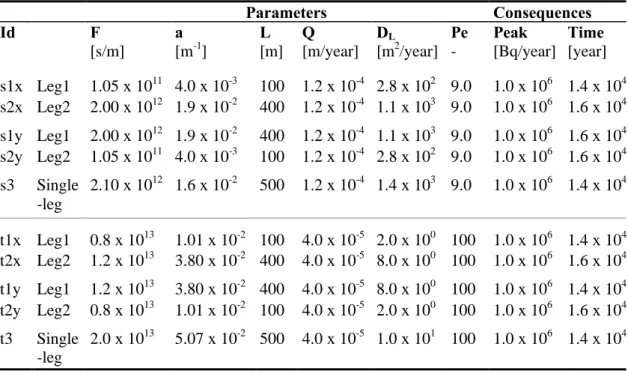
Table III Case A0. Input data and results for the double-leg simulations with varying
flow-wetted surface area and longitudinal dispersion for a stable nuclide. The distribution coefficient is zero. DL is proportional to the leg length.
Parameters Consequences Id F [s/m] a [m-1] L [m] Q [m/year] DL [m2/year] Pe -Peak [Bq/year] Time [year] s1x Leg1 1.05 x 10¹¹ 4.0 x 10⁻³ 100 1.2 x 10⁻⁴ 2.8 x 10² 9.0 1.0 x 10⁶ 1.4 x 10⁴ s2x Leg2 2.00 x 10¹² 1.9 x 10⁻² 400 1.2 x 10⁻⁴ 1.1 x 10³ 9.0 1.0 x 10⁶ 1.6 x 10⁴ s1y Leg1 2.00 x 10¹² 1.9 x 10⁻² 400 1.2 x 10⁻⁴ 1.1 x 10³ 9.0 1.0 x 10⁶ 1.6 x 10⁴ s2y Leg2 1.05 x 10¹¹ 4.0 x 10⁻³ 100 1.2 x 10⁻⁴ 2.8 x 10² 9.0 1.0 x 10⁶ 1.6 x 10⁴ s3 Single -leg 2.10 x 10¹² 1.6 x 10⁻² 500 1.2 x 10⁻⁴ 1.4 x 10³ 9.0 1.0 x 10⁶ 1.4 x 10⁴ t1x Leg1 0.8 x 10¹³ 1.01 x 10⁻² 100 4.0 x 10⁻⁵ 2.0 x 100 100 1.0 x 10⁶ 1.4 x 10⁴ t2x Leg2 1.2 x 10¹³ 3.80 x 10⁻² 400 4.0 x 10⁻⁵ 8.0 x 100 100 1.0 x 10⁶ 1.6 x 10⁴ t1y Leg1 1.2 x 10¹³ 3.80 x 10⁻² 400 4.0 x 10⁻⁵ 8.0 x 100 100 1.0 x 10⁶ 1.4 x 10⁴ t2y Leg2 0.8 x 10¹³ 1.01 x 10⁻² 100 4.0 x 10⁻⁵ 2.0 x 100 100 1.0 x 10⁶ 1.6 x 10⁴ t3 Single -leg 2.0 x 10¹³ 5.07 x 10⁻² 500 4.0 x 10⁻⁵ 1.0 x 101 100 1.0 x 10⁶ 1.4 x 10⁴ †
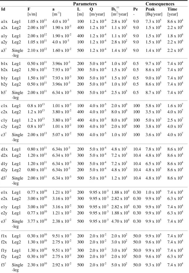
Table IV Case A1. Input data and results for the double-leg simulations with varying
flow-wetted surface area and longitudinal dispersion for a stable nuclide. The distribution coefficient is equal to 1.0 m3/kg. DL is proportional to the leg length.
Parameters Consequences Id F [s/m] a [m-1] L [m] Q [m/year] DL†† [m2/year] Pe -Peak [Bq/year] Time [year] a1x Leg1 1.05 x 10¹¹ 4.0 x 10⁻³ 100 1.2 x 10⁻⁴ 2.8 x 10² 9.0 7.3 x 10⁵ 8.6 x 10⁴ a2x Leg2 2.00 x 10¹² 1.90 x 10⁻² 400 1.2 x 10⁻⁴ 1.1 x 10³ 9.0 1.5 x 10⁴ 2.2 x 10⁶ a1y Leg1 2.00 x 10¹² 1.90 x 10⁻² 400 1.2 x 10⁻⁴ 1.1 x 10³ 9.0 1.5 x 10⁴ 1.8 x 10⁶ a2y Leg2 1.05 x 10¹¹ 4.0 x 10⁻³ 100 1.2 x 10⁻⁴ 2.8 x 10² 9.0 1.5 x 10⁴ 2.2 x 10⁶ a3† Single -leg 2.10 x 10¹² 1.60 x 10⁻² 500 1.2 x 10⁻⁴ 1.4 x 10³ 9.0 1.4 x 10⁴ 2.2 x 10⁶ b1x Leg1 0.50 x 10¹¹ 3.96x 10⁻³ 200 5.0 x 10⁻⁴ 1.0 x 10⁵ 0.5 9.7 x 10⁵ 7.4 x 10⁴ b2x Leg2 1.50 x 10¹¹ 7.93 x 10⁻³ 300 5.0 x 10⁻⁴ 1.5 x 10⁵ 0.5 8.6 x 10⁵ 7.4 x 10⁴ b1y Leg1 1.50 x 10¹¹ 7.93 x 10⁻³ 300 5.0 x 10⁻⁴ 1.5 x 10⁵ 0.5 9.0 x 10⁵ 7.4 x 10⁴ b2y Leg2 0.50 x 10¹¹ 3.96x 10⁻³ 200 5.0 x 10⁻⁴ 1.0 x 10⁵ 0.5 8.6 x 10⁵ 7.4 x 10⁴ b3† Single -leg 2.00 x 10¹¹ 6.34 x 10⁻³ 500 5.0 x 10⁻⁴ 2.5 x 10⁵ 0.5 8.7 x 10⁵ 7.4 x 10⁴ c1x Leg1 0.8 x 10¹³ 1.01 x 10⁻² 100 4.0 x 10⁻⁵ 2.0 x 100 100 5.8 x 10³ 1.6 x 10⁷ c2x Leg2 1.2 x 10¹³ 3.80 x 10⁻² 400 4.0 x 10⁻⁵ 8.0 x 100 100 3.5 x 10³ 4.0 x 10⁷ c1y Leg1 1.2 x 10¹³ 3.80 x 10⁻² 400 4.0 x 10⁻⁵ 8.0 x 100 100 5.0 x 10³ 2.5 x 10⁷ c2y Leg2 0.8 x 10¹³ 1.01 x 10⁻² 100 4.0 x 10⁻⁵ 2.0 x 100 100 3.8 x 10³ 4.0 x 10⁷ c3† Single -leg 2.00 x 10¹³ 5.07 x 10⁻² 500 4.0 x 10⁻⁵ 1.0 x 101 100 3.6 x 10³ 4.0 x 10⁷ d1x Leg1 0.80 x 10¹¹ 6.34x 10⁻³ 200 5.0 x 10⁻⁴ 4.8 x 10³ 10.4 7.8 x 10⁵ 8.6 x 10⁴ d2x Leg2 1.20 x 10¹¹ 6.34 x 10⁻³ 300 5.0 x 10⁻⁴ 7.2 x 10³ 10.4 4.8 x 10⁵ 8.6 x 10⁴ d1y Leg1 1.20 x 10¹¹ 6.34 x 10⁻³ 300 5.0 x 10⁻⁴ 7.2 x 10³ 10.4 6.5 x 10⁵ 8.6 x 10⁴ d2y Leg2 0.80 x 10¹¹ 6.34x 10⁻³ 200 5.0 x 10⁻⁴ 4.8 x 10³ 10.4 4.8 x 10⁵ 8.6 x 10⁴ d3† Single -leg 2.00 x 10¹¹ 6.34 x 10⁻³ 500 5.0 x 10⁻⁴ 1.2 x 10⁴ 10.4 4.8 x 10⁵ 8.6 x 10⁴ e1x Leg1 0.77 x 10¹⁰ 1.21 x 10⁻² 200 9.95 x 10⁻³ 1.88 x 10⁴ 0.30 1.0 x 10⁶ 7.4 x 10⁴ e2x Leg2 3.00 x 10¹⁰ 3.16 x 10⁻² 300 9.95 x 10⁻³ 2.82 x 10⁴ 0.30 9.9 x 10⁵ 6.3 x 10⁴ e1y Leg1 3.00 x 10¹⁰ 3.16 x 10⁻² 300 9.95 x 10⁻³ 2.82 x 10⁴ 0.30 9.9 x 10⁵ 7.4 x 10⁴ e2y Leg1 0.77 x 10¹⁰ 1.21 x 10⁻² 200 9.95 x 10⁻³ 1.88 x 10⁴ 0.30 9.9 x 10⁵ 6.3 x 10⁴ e3† Single -leg 3.77 x 10¹⁰ 2.38 x 10⁻² 500 9.95 x 10⁻³ 4.70 x 10⁴ 0.30 9.9 x 10⁵ 7.4 x 10⁴ f1x Leg1 0.30 x 10¹⁰ 9.51 x 10⁻³ 200 2.0 x 10⁻² 2.0 x 10² 50.0 9.9 x 10⁵ 7.4 x 10⁴ f2x Leg2 1.30 x 10¹⁰ 2.75 x 10⁻² 300 2.0 x 10⁻² 3.0 x 10² 50.0 9.6 x 10⁵ 7.4 x 10⁴ f1y Leg1 1.30 x 10¹⁰ 9.51 x 10⁻³ 300 2.0 x 10⁻² 3.0 x 10² 50.0 9.9 x 10⁵ 7.4 x 10⁴ f2y Leg2 0.30 x 10¹⁰ 2.75 x 10⁻² 200 2.0 x 10⁻² 2.0 x 10² 50.0 9.6 x 10⁵ 6.3 x 10⁴ f3† Single -leg 2.30 x 10¹⁰ 2.92 x 10⁻² 500 2.0 x 10⁻² 5.0 x 10² 50.0 9.3 x 10⁵ 7.4 x 10⁴ †
The data of the rows a3, b3, c3, d3, e3 and f3 correspond to that of cases FF0, FF37, FF4, FF17, FF41 and FF6 of the SITE-94 project.
Figure 5 The breakthrough curves for the single and double-leg models (s3) and (s2x
and s2y) respectively for a low Peclet number and with the distribution coefficient equal to zero.
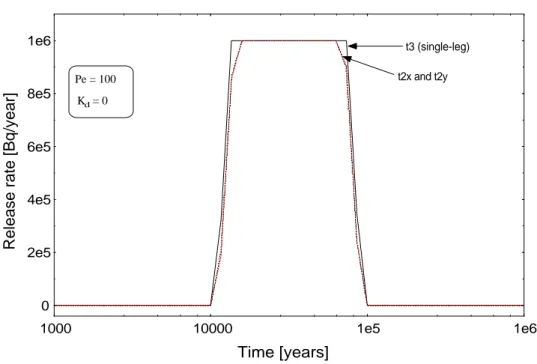
Figure 6 The breakthrough curves for the single and double-leg models (t3) and (t2x
and t2y) respectively for the case of a high Peclet number and with the distribution
coefficient equal to zero.
Time [years]
Release rate [Bq/year]
0 2e5 4e5 6e5 8e5 1e6 1000 10000 1e5 1e6 s3 (single-leg) Pe = 9 Kd = 0 s2x and s2y Time [years]
Release rate [Bq/year]
0 2e5 4e5 6e5 8e5 1e6 1000 10000 1e5 1e6 Pe = 100 Kd = 0 t3 (single-leg) t2x and t2y
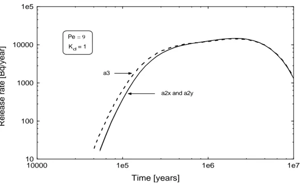
Figure 7 The breakthrough curves for the single and the double-leg models (a3)
and (a2x and a2y) respectively for a low Peclet number and with the distribution coefficient equal to one.
Figure.8 The breakthrough curves for the single and double-leg models (c3)
and (c2x and c2y) respectively for the case of a high Peclet number and with the distribution coefficient equal to one.
Time [years]
Release rate [Bq/year]
10 100 1000 10000 1e7 1e8 Pe = 100 c2y c2x and c3 Kd = 1 5e7 Time [years]
Release rate [Bq/year]
10 100 1000 10000 1e5
10000 1e5 1e6 1e7
Pe = 9
a2x and a2y a3
4.1.2 The impact of the F-ratio with the Peclet numbers varying along the path −− Case A2.
In this section we use the double-leg model to illustrate the consequences of departure from the assumption that the longitudinal dispersion of different legs adds to the value of the longitudinal dispersion for the single-leg model. The aim is to motivate why we need to use the additivity assumption for the longitudinal dispersion throughout the calculations.
The Peclet number gives the ratio between characteristic times for the diffusive and advective processes:
where q [m/year] is the Darcy velocity, L [m] is the transport length, 2 [-] is the flow
porosity and DL [m2/year] is the longitudinal dispersion coefficient. If the longitudinal
dispersions are not additive, the Peclet number is no longer the same for the single-leg model and the multiple-leg model. This will influence the outcome of the simulations in such a way that it can balance or reinforce the impact of the F-ratio, as will be shown by the results.
Table V shows the input data and the results. The half-life was set to infinity, i.e., we
simulate a non-decaying species. The reader should note that the case given in row g
(single-leg), i.e., the simulation for the total path length L, has one far-field parameter which is different of that of case FF0 from SITE-94. This is the longitudinal dispersion, which is 1.25 x 10⁵ m2/year instead of 1.4 x 10³ m2/year. The former value is the mean value for the longitudinal dispersions of the two legs, which are now different.
The Table V shows that for simulations (g1,g2) and (g1x, g2x), there is a discrepancy
between the peak releases of more than one order of magnitude compared to case g
(single-leg), even though all cases have the same total F-ratio. Figure 5 in Appendix II
shows that the breakthrough curves are clustered into two groups. Case g (single-leg) together with cases g2y and g2z forms one cluster with a peak release of roughly 7.0 x
105 Bq/year, while cases g2 and g2x form another cluster with a peak release equal to
1.5 x 10⁴ Bq/year.
Because we have departed from the assumption that the longitudinal dispersion should
be proportional to the lengths of the two legs, we face the question: what DL value
should we use for the corresponding single-leg model? The value of DL that was chosen,
was the mean value for the two legs, as pointed out before. But, even if the above choice
of DL value for the single-leg model is arbitrary, the nature of the discrepancy cannot be
removed by making another choice. Suppose, for instance, that one was able to tune the
choice of DL value for the single-model in such a way that the peak releases for the
simulations given by rows g2 and g2x in Table V were almost equal to that for row g,
i.e., by the single-leg model. Then the value given in row g should be approximately
equal to 1.5x10⁴ Bq/year instead of 6.8 x 10⁵ Bq/year and the peak releases given by
rows g2y and g2z would differ considerably from those given by the single-leg model.
(4)
L D qL Pe= θ
Table V Case A2. Input data and results for the double-leg simulations with
flow-wetted surface area, longitudinal dispersion and Peclet numbers varying along the transport pathway. Parameters Consequences Id F [s/m] a [m-1] L [m] Q [m/year] DL [m2/year] Pe [-] Peak [Bq/year] Time [year] g1 Leg1 1.05 x 10¹¹ 4.0 x 10⁻³ 100 1.2 x 10⁻⁴ 2.5 x 10⁵ 0.01 9.9 x 10⁵ 7.4 x 10⁶ g2 Leg2 2.00 x 10¹² 1.9 x 10⁻² 400 1.2 x 10⁻⁴ 1.4 x 10³ 6.9 1.5 x 10⁴ 1.6 x 10⁶ g1x Leg1 2.00 x 10¹² 4.0 x 10⁻³ 400 1.2 x 10⁻⁴ 1.4 x 10³ 6.9 1.5 x 10⁴ 1.6 x 10⁸ g2x Leg2 1.05 x 10¹¹ 1.9 x 10⁻² 100 1.2 x 10⁻⁴ 2.5 x 10⁵ 0.01 1.5 x 10⁴ 1.6 x 10⁸ g1y Leg1 1.05 x 10¹¹ 4.0 x 10⁻³ 100 1.2 x 10⁻⁴ 1.4 x 10³ 1.7 8.3 x 10⁵ 7.4 x 10⁴ g2y Leg2 2.00 x 10¹² 1.9 x 10⁻² 400 1.2 x 10⁻⁴ 2.5 x 10⁵ 0.04 7.1 x 10⁵ 7.4 x 10⁴ g1z Leg1 2.00 x 10¹² 1.9 x 10⁻² 400 1.2 x 10⁻⁴ 2.5 x 10⁵ 0.04 8.8 x 10⁵ 7.4 x 10⁴ g2z Leg2 1.05 x 10¹¹ 4.0 x 10⁻³ 100 1.2 x 10⁻⁴ 1.4 x 10³ 1.7 7.1 x 10⁵ 7.4 x 10⁴ g† Single -leg 2.01 x 10¹² 1.6x 10⁻² 500 1.2 x 10⁻⁴ 1.25 x 10⁵ 0.1 6.8 x 10⁵ 8.5 x 10⁴ †
The data in this row correspond to the FF0 case, with exception of the longitudinal dispersion, which is the arithmetic mean of that of legs 1and 2.
We conclude that for case A2, even if the sum of the F-ratios for the sets of simulations using the double-leg model is equal to the F-ratio of the single-leg model, we do not obtain close results. The fact that the longitudinal dispersions are not proportional to the length of the legs leads to very distinct breakthrough curves with peak releases that can differ by more than one order of magnitude.
Hence, the F-ratio can no longer be interpreted (in the context of the double-leg model)
as a resistance offered by the rock to groundwater flow, though F is still equal to the
sum of the partial Fi´s. Or, expressed in other words, the additivity property of the
F-ratio does not lead to similar breakthrough curves. This conclusion motivates the assumption of using a constant Peclet number along the transport pathway in this work, i.e., the longitudinal dispersion must be proportional to the transport pathway length.
4.2 The ten-leg model: Results and discussion
4.2.1 Stable species
−−
Case B1
From now on we will only use an extension of the double-leg model obtained by increasing the number of legs to 10. The input data for and the results of this model pertaining to the case B1 are shown in Table VI below. The radioactive decay is not considered, i.e., we have a stable species. The longitudinal dispersions in the ten-leg model are proportional to the path length of each leg. This assumption means that longitudinal dispersion of the equivalent “single-leg” model is equal to the sum of the longitudinal dispersions for all legs:
Equation 5 expresses the assumed additivity of dispersions, which, together with Eqn. 6
results in equivalent breakthrough curves for the single-leg model and the ten-leg model (figure 9), showing that also in this case the formulations of the flow problem are equivalent and the F-ratio can be interpreted as being the resistance offered by the rock to groundwater flow.
Table VI Case B1. Input data and results for ten-leg simulations with varying
flow-wetted surface area. Stable species.
Id F [S/m] a [m-1] L [m] Q [m/year] DL [m2/year] Pe [-] Peak [Bq/year] Time [year] h1 Leg1 1.40 x 10¹¹ 8.88 x 10⁻² 60 1.2 x 10⁻³ 1.7x 10² 8.6 x 101 5.67 x 10⁵ 8.6 x 10⁴ h2 Leg2 2.40 x 10¹¹ 2.03 x 10⁻¹ 45 1.2 x 10⁻³ 1.3 x 10² 8.6 x 101 1.89 x 10⁵ 1.4 x 10⁵ h3 Leg3 4.00 x 10¹¹ 3.71 x 10⁻¹ 41 1.2 x 10⁻³ 1.1 x 10² 8.6 x 101 5.02 x 10⁴ 2.9 x 10⁵ h4 Leg4 1.00 x 10¹¹ 9.51 x 10⁻² 40 1.2 x 10⁻³ 1.1 x 10² 8.6 x 101 3.98 x 10⁴ 4.0 x 10⁵ h5 Leg5 1.00 x 10⁹ 1.23 x 10⁻² 31 1.2 x 10⁻³ 8.7x 101 8.6 x 101 3.91 x 10⁴ 4.0 x 10⁵ h6 Leg6 8.00 x 10¹¹ 6.66 x 10⁻¹ 40 1.2 x 10⁻³ 1.1x 10² 8.6 x 101 1.22 x 10⁴ 1.2 x 10⁵ h7 Leg7 3.10 x 10¹¹ 1.82 x 10⁻¹ 65 1.2 x 10⁻³ 1.8x 10² 8.6 x 101 8.69 x 10³ 1.6 x 10⁶ h8 Leg8 1.00 x 10¹⁰ 1.59 x 10⁻² 48 1.2 x 10⁻³ 1.3 x 10² 8.6 x 101 8.38 x 10³ 1.9 x 10⁶ h9 Leg9 9.90 x 10¹⁰ 5.07 x 10⁻² 60 1.2 x 10⁻³ 1.7x 10² 8.6 x 101 7.84 x 10³ 1.6 x 10⁶ h10 Leg10 1.10 x 10¹¹ 5.44 x 10⁻² 70 1.2 x 10⁻³ 2.0x 10² 8.6 x 101 7.15 x 10³ 1.8 x 10⁶ h11 Single -leg 2.10x 10¹² 1.60 x 10⁻¹ 500 1.2 x 10⁻³ 1.4 x 10³ 8.6 x 101 6.74 x 10³ 1.8 x 10⁶ ∑ = i Li L D D (5) ) 6 ( ∑ = i iF F
Figure 9 Ten-leg calculations with varying flow-wetted surface area compared with
the equivalent single-leg model. The calculations assume a stable species.
4.2.2 Decaying species
−−
Case B2
What will happen if one introduces decaying species? To assess this, we made
deterministic simulations based on data from case B1 given in Table VI (see also Table 5 in Appendix I) but with Kd and T1/2 as given in Table VII.
In a variant of the ten-leg simulation, the results of which are shown in Fig. 10, we use a
radionuclide with a half-life equal to 7.38x10³.The input data are equal to that of Table
VI, with the exception of the half-life as mentioned above. The results now disagree by
eight orders of magnitude. As in the previous cases, the Kd parameter is equal to 1.0
[m3/kg ], which is rather high. Nevertheless in the cases of stable species it had no
influence on the differences between the ten-leg model and the single-leg model.
Increasing the half-life of the species by one order of magnitude (to 7.38x10⁴), but
keeping the Kd equal to 1.0 m3/kg, results in a disagreement of two orders of magnitude
(Fig. 12). Decreasing the Kd by one order of magnitude to 0.1 m3/kg, reduced the
discrepancy between the two models to about one-half an order of magnitude (Fig. 11). Finally, with Kd equal to 0.1 m3/kg and T1/2 equal to 7.38x10³ the disagreement
increases to more than two orders of magnitude (Fig. 13). The results of these variations are summarised in Table VII.
Time [years]
Release rate [Bq/year]
10 100 1000 10000
1e5 1e6 1e7
Single-leg model
Ten-leg model Kd=1.0
Table VII Case B2. Results of parameter variations for single and ten-leg simulations
with varying flow-wetted surface area for stable and decaying species.
Id† K d [m3/kg] T ½ [year] Single-leg Ten-leg Peak [Bq/year] Time [year] Peak [Bq/year] Time [year] Figure nr. 1 1.0 4 ¥ 6.74 x 10³ 1.8 x 10⁶ 7.15 x 10³ 1.8 x 10⁶ 9 2 1.0 7.4 x 10³ 1.27 x 10⁻⁵ 1.4 x 10⁵ 1.11 x 10³ 1.6 x 10⁶ 10 3 0.1 7.4 x 10⁴ 1.95 x 10⁴ 1.6 x 10⁵ 6.66 x 10⁴ 2.5 x 10⁵ 11 4 1.0 7.4 x 10⁴ 2.05 x 101 4.0 x 10⁵ 4.17 x 10³ 1.6 x 10⁶ 12 5 0.1 7.4 x 10³ 9.59 x 101 1.0 x 10⁵ 4.88 x 10⁴ 2.1 x 10⁵ 13 6 0 7.4 x 10³ 9.98 x 10⁵ 1.4 x 10⁴ 9.93 x 10⁵ 2.5 x 10⁴ 6‡‡ †
Here the data set of Table VI is used with different values for the half-life and Kd.
‡‡
Appendix II.
It is clear that the F-ratios do not represent a resistance for the transport problem simulated by the ten-leg model if the distribution coefficient is different from zero and the half-live of the nuclide has a finite value (the case with a distribution coefficient equal to zero is illustrated in Figure 6 of Appendix II). Indeed, the additivity property of the F-ratio does not lead to similar breakthrough curves for the single-leg and ten-leg model. In other words, the F-ratio is a resistance offered by the rock to the groundwater flow, but not a resistance to radionuclide transport, which is also confirmed in Section 5.2 where the chemistry is allowed to vary along the transport pathway.
Figure 10 Ten-leg calculations with varying flow-wetted surface area and
longitudinal dispersion compared with the equivalent single-leg model. In this calculation the Kd value of the decaying species is equal to 1.0 m3
/kg as in the
previous calculation. Note that the y-scale has been extended to very low values to include the single-leg model breakthrough curve.
Figure 11 Ten-leg calculations with varying flow-wetted surface area and longitudinal
dispersion compared with the equivalent single-leg model. In this calculation the Kd value of the decaying species is as in the previous one equal to 1.0 m3
/kg but the
half-life has been increased by one order of magnitude.
Time [years]
Release rate [Bq/year]
10 100 1000 10000 1e5
10000 1e5 1e6 1e7
Kd=0.1 T1/2=7.38 x 104
Single-leg model Ten-leg model
Time [years]
Release rate [Bq/year]
1e-6 1e-4 0,01 1 100 10000
10000 1e5 1e6 1e7
Kd = 1.0
Single-leg model Ten-leg model T1/2=7.38 x 103
Figure 12 Ten-leg calculations with varying flow-wetted surface area and longitudinal
dispersion compared with the equivalent single-leg model. In this calculation the Kd value had been decreased by one order of magnitude to 0.1 m3
/kg.
Figure 13 Ten-leg calculations with varying flow-wetted surface area and longitudinal
dispersion compared with the equivalent single-leg model.
Time [years]
Release Rate [Bq/year]
10 100 1000 10000 1e5
10000 1e5 1e6 1e7
Kd = 0.1 T1/2 =7.38 x 10 3 Single-leg model Ten-leg model Time [years]
Release rate [Bq/year]
10 100 1000 10000
1e5 1e6 1e7
Kd=1.0
Single-leg model
Ten-leg model T1/2=7.38 x 10
5. The impact of the F-ratio on radionuclide release
for simultaneous variations in the flow and transport
parameters
5.1 Introduction
In Section Four we addressed the impact of the F-ratio whenever one only considers the spatial variability of the flow parameters that enter in the transport model. The goal was to determine the conditions of validity for the interpretation of the F-ratio for a
multiple-leg model as a transport resistance of the rock to the groundwater movement. And in its sequence the possibility of using information from site characterisation to reduce the uncertainties of the flow parameters needed for the transport calculations. In this section we deal with the fully coupled model with the goal now being to study the impact of the F-ratio in simulations subjected to simultaneous variability of both flow and transport parameters. Are there any significative differences in the results, in between using a fully coupled model that takes the intrinsic variability of all parameters into account (multiple-leg model) and a model that cannot cope with that variability (single-leg model)?
5.2 The fully coupled transport model
−−
Case B3
In the previous section the Kd parameter was assumed to be constant along the transport
pathway. The variation in the mineralogy along the pathway makes it necessary to
include Kd variations from block to block. The input data used to make simulations for
this case (Table VIII) are the same as those shown in Table VI, apart from a difference
related to the distribution coefficients. These were allowed to vary from 1x10⁻⁴ to 0.1
m3/kg. It is not, therefore, obvious which Kd one should use for the single-leg model for
comparison purposes. Thus we have used both the mean and the median of the Kd
values of the ten legs.
The results are displayed in Fig. 14, showing that the single-leg model can be either
conservative or optimistic, depending upon the Kd used (Table IX). For median values
we obtain a pessimistic estimate of the peak release, while the use of the mean value results in a slightly optimistic estimation. The shape of the breakthrough curve for the ten-leg model differs considerably from the mean and median breakthrough curves of the single-leg model.
Table VIII Case B3. Input data for 10-leg simulations with varying flow-wetted surface area, longitudinal dispersion
and sorption coefficient. Decaying species, with T1/2 = 7.38 x 10⁴years.
Id F [S/m] a [m-1] L [m] Q [m/year] DL [m2/year] Pe [-] Kd [m3/kg] Peak [Bq/year] Time [year] i1 Leg1 1.4 x 10¹¹ 8.88 x 10⁻² 60 1.2 x 10⁻³ 1.7x 10² 8.6 x 101 1.0 x 10⁻² 9.3 x 10⁵ 7.3 x 10⁴ i2 Leg2 2.4 x 10¹¹ 2.03 x 10⁻¹ 45 1.2 x 10⁻³ 1.3 x 10² 8.6 x 101 5.0 x 10⁻² 7.5 x 10⁵ 7.4 x 10⁴ i3 Leg3 4.0 x 10¹¹ 3.71 x 10⁻¹ 41 1.2 x 10⁻³ 1.1 x 10² 8.6 x 101 1.0 x 10⁻³ 7.2 x 10⁵ 7.4 x 10⁴ i4 Leg4 1.0 x 10¹¹ 9.51 x 10⁻² 40 1.2 x 10⁻³ 1.1 x 10² 8.6 x 101 1.1 x 10⁻¹ 6.9 x 10⁵ 7.4 x 10⁴ i5 Leg5 1.0 x 10⁹ 1.23 x 10⁻² 31 1.2 x 10⁻³ 8.7x 101 8.6 x 101 1.0 x 10⁻⁴ 6.8 x 10⁵ 7.4 x 10⁴ i6 Leg6 8.0 x 10¹¹ 6.66 x 10⁻¹ 40 1.2 x 10⁻³ 1.1x 10² 8.6 x 101 5.0 x 10⁻¹ 8.6 x 10⁴ 2.2 x 10⁵ i7 Leg7 3.1 x 10¹¹ 1.82 x 10⁻¹ 65 1.2 x 10⁻³ 1.8x 10² 8.6 x 101 2.0 x 10⁻² 7.5 x 10⁴ 2.2 x 10⁵ i8 Leg8 1.0 x 10¹⁰ 1.59 x 10⁻² 48 1.2 x 10⁻³ 1.3 x 10² 8.6 x 101 2.6 x 10⁻² 7.4 x 10⁴ 2.2 x 10⁵ i9 Leg9 9.9 x 10¹⁰ 5.07 x 10⁻² 60 1.2 x 10⁻³ 1.7x 10² 8.6 x 101 2.7 x 10⁻³ 7.4 x 10⁴ 2.2 x 10⁵ i10 Leg10 1.1 x 10¹¹ 5.44 x 10⁻² 70 1.2 x 10⁻³ 2.0x 10² 8.6 x 101 7.1 x 10⁻² 6.9 x 10⁴ 2.5 x 10⁵ i11a Single -leg 2.1x 10¹² 1.60 x 10⁻¹ 500 1.2 x 10⁻³ 1.4 x 10³ 8.6 x 101 7.9 x10⁻² † 2.9 x 10⁴ 1.6 x 10⁵ i11b Single -leg 2.1x 10¹² 1.60 x 10⁻¹ 500 1.2 x 10⁻³ 1.4 x 10³ 8.6 x 101 2.3 x 10⁻² ‡ 1.5 x 10⁵ 1.0 x 10⁵ †
This value is the mean of the Kd values for the ten legs.
‡
Table IX Case B3. Résumé of the results obtained from calculations with
input data from Table VIII.
Model Id Kd [m3/kg] Peak [Bq/year] Time [year]
Ten-leg i10 variable† 6.9 x 10⁴ 2.5 x 10⁵
i11a Mean 2.9 x 10⁴ 1.6 x 10⁵
Single-leg
i11b Median 1.5 x 10⁵ 1.0 x 10⁵
†
These variations in Kd are taken based upon the data set of Table VI. T1/2 = 7.38 x 10⁴
years.
Figure 14 Ten-leg calculations with varying flow-wetted surface area, longitudinal
dispersion and Kd. The equivalent single-leg model is displayed for comparison.
It is clear that the F-ratio of a multiple-leg model in the case of simultaneous variation of flow and transport parameters is not a resistance to radionuclide transport. Maybe, for the set of parameters used here, the differences in peak values are relatively small, but the resulting shapes of the single-leg model breakthrough curves result in dramatic differences between the tails of those curves and that of the ten-leg model curve.
Time [years]
Release rate [Bq/year]
100 1000 10000 1e5 1e6 10000 1e5 1e6 Ten-leg model Single-leg: mean distribution coefficient Single-leg: median distribution coefficient
6. Summary and conclusions
A large number of deterministic calculations have been made to study the impact of the F-ratio on the calculated results for radionuclide transport in the geosphere. The object of the investigation is to examine the additivity of the F-ratio and the consequent interpretation of the sum of F-ratios - for different paths connected in series - as a transport resistance for groundwater flow. Ultimately its importance is related to the treatment of 3D data from site characterisation and its reduction to effective flow parameters to be used in 1D transport models for the performance assessment (the first of the aims within this work) and also to examine the capabilities required for the next generation of PA transport codes.
To attain our goal, a multiple-leg model was set up, based upon the one-dimensional CRYSTAL transport model. From transport calculations performed with CRYSTAL using a single transport pathway, we know that the F-ratio can be interpreted as a transport resistance to groundwater flow. If we want to incorporate the intrinsic spatial variability of parameters in a model, the question arises of whether the F-ratio is still a transport resistance. If so, the resistance offered by the different legs of, for instance a
multiple-leg code, should sum to the resistance for the equivalent single-model, i.e., F
should also be additive for such a model. The only way to vary the parameters along the transport pathway using CRYSTAL is to set up a multiple-leg model where each leg is representative of a characteristic rock block with its own properties given by averaged parameters.
It is known from transport calculations of migration in heterogeneous fractured rock using 1D codes like CRYSTAL that roughly speaking three important groups of parameters are involved, two of them dealing with the “flow problem” and the third with the chemical interaction of the radionuclides with the host rock. The first two groups are given by the F-ratio and the Peclet number and the third by surface or/and matrix retardation (in general using the linear retention coefficient Kd ). This
information was used in this work to formulate the different cases needed to analyse the impact of the F-ratio in multiple-leg models.
Two variants of the multiple-leg model are used in the calculations: a double-leg model and a ten-leg model. The results of these two models are compared with the results for an equivalent single-leg model.
From the calculations it was verified that the F-ratio can still be interpreted as a transport resistance for stable species if the F-ratio is additive and if an extra condition is imposed on the longitudinal dispersion. This condition indicates that the longitudinal dispersion should also be an additive parameter, i.e., the longitudinal dispersion for each of the different legs of the multiple-leg model should sum to the longitudinal dispersion for the equivalent single-leg model. This last condition is necessary, but not sufficient. Indeed the longitudinal dispersions for the different legs should also be proportional to the path lengths. The above conclusion is valid for 1D formulations of transport models with a mathematical structure akin to that of CRYSTAL, i.e., advective-dispersive--reactive models. From this conclusion it follows that, assuming the above conditions, it is possible to use site characterisation to extract very useful information regarding flow parameters that can be used for 1D models.
The second goal of this report was to examine the impact of the F-ratio on the results of the fully coupled transport model. From the calculations it can be concluded that for decaying species, even considering the additivity of longitudinal dispersion, the F-ratio is not a good representation of the “total” resistance in a multiple-leg model. Or, in other words, whenever heterogeneity is taken into account in the multiple-leg transport models, the F-ratio is a transport resistance for the groundwater flow, but not a transport resistance for solute mass transport. Indeed it is shown that for the fully coupled model, deterministic calculations with single-leg models can come up with either optimistic or
pessimistic results depending on the choice of parameters, the Kd value being
particularly sensitive for the CRYSTAL model if one compares with the results of the multiple-leg model. The shape of breakthrough curves is also very different from each other. The non-ability of the single-leg transport model to cope with spatial variability has consequences in probabilistic calculations also. Even if reasons other than those examined in this report come into play, the calculations done for the second part of this report reinforce the previous conclusions from probabilistic calculations, namely that, for Monte Carlo calculations (Pereira et al., 1997), new tools which can cope with intrinsic spatial variability of parameters are needed.
References
1. Robinson, P. and Worgan, K. (1992). CRYSTAL: A Model of Fractured Rock
Geosphere for Performance Assessment within the SKI Project-90. SKI Technical
Report 91:13, Stockholm, Sweden.
2. SKI, Project-90, SKI TR 91:23, Swedish Nuclear Power Inspectorate, Stockholm, 1991.
3. SKI SITE-94, Deep Repository Performance Assessment Project, 1996. SKI Report 96:13, Sweden.
4. Neretnieks, I., Abelin, H. and Birgersson, L., 1987. Some recent observations of
channelling in fractured rocks – Its potential impact on radionuclide migration. In:
U. S. Dep. Energy –At. Energy Can. Lab. Conf., Sept 15-17, 1987, San Francisco, CA,Proc., pp. 387-410.
5. Andersson, M., Mendes, B., and Pereira, A. (1997). The Impact of Heterogeneity of
Fractured Media in Monte Carlo Assessments of High-Level Nuclear Waste. A Comparative Study (CD-ROM: Proceedings of the WM´97 Conference, Tucson,
Arizona, USA).
6. A. Pereira, M. Andersson and B. Mendes (1997). Parallel Computing in
Probabilistic Safety Assessments of High-Level Nuclear Waste. Advances in Safety
and Reliability (Ed. C. Guedes Soares, Pergamon), Proc. of the Esrel´97 Int. Conf. on Safety and Reliability, Lisbon, Portugal, pp 585-592.
Appendix I
Table 1 Test case. The input parameters for the double-leg model are equal to those of the single-leg model
with the exception of the transport distances of legs 1 and 2.
Parameters
Id a [m-1] L [m] Q [m/year] DL [m2/year] ggf [-] Dm [m2/year] Pdepth [m] S [m] ggp [-] Kd [m3/kg] v1x Leg1 1.6 x 10⁻² 250 1.2 x 10⁻⁴ 1.4 x 10³ 5.0 x 10⁻⁶ 9.5 x 10⁻³ 5.0 x 10⁻¹ 1.0 1.0 x 10⁻³ 1.0 v2x Leg2 1.6 x 10⁻² 250 1.2 x 10⁻⁴ 1.4 x 10³ 5.0 x 10⁻⁶ 9.5 x 10⁻³ 5.0 x 10⁻¹ 1.0 1.0 x 10⁻³ 1.0 v3 Single-leg 1.6 x 10⁻² 500 1.2 x 10⁻⁴ 1.4 x 10³ 5.0 x 10⁻⁶ 9.5 x 10⁻³ 5.0 x 10⁻¹ 1.0 1.0 x 10⁻³ 1.0Table 2 Case A0. Input parameters for the double-leg calculations with constant Peclet numbers.
Parameters
Id F [s/m] a [m-1] L [m] Q [m/year] DL†† [m2/year] Pe [-] ggf [-] Dm [m2/year] Pdepth [m] S [m] [-]ggp Kd [m3/kg] s1x Leg1 1.05 x 10¹¹ 4.00 x 10⁻³ 100 1.2 x 10⁻⁴ 2.8 x 10² 9.0 5.0 x 10⁻⁶ 9.5 x 10⁻⁴ 5.0 x 10⁻² 1.0 1.0 x 10⁻³ 1.0 s2x Leg2 2.00 x 10¹² 1.90 x 10⁻² 400 1.2 x 10⁻⁴ 1.1 x 10³ 9.0 5.0 x 10⁻⁶ 9.5 x 10⁻⁴ 5.0 x 10⁻² 1.0 1.0 x 10⁻³ 1.0 s1y Leg1 2.00 x 10¹² 1.90 x 10⁻² 400 1.2 x 10⁻⁴ 1.1 x 10³ 9.0 5.0 x 10⁻⁶ 9.5 x 10⁻⁴ 5.0 x 10⁻² 1.0 1.0 x 10⁻³ 1.0 s2y Leg2 1.05 x 10¹¹ 4.00 x 10⁻³ 100 1.2 x 10⁻⁴ 2.8 x 10² 9.0 5.0 x 10⁻⁶ 9.5 x 10⁻⁴ 5.0 x 10⁻² 1.0 1.0 x 10⁻³ 1.0 s3 Single -leg 2.10 x 10¹² 1.60 x 10⁻² 500 1.2 x 10⁻⁴ 1.4 x 10³ 9.0 5.0 x 10⁻⁶ 9.5 x 10⁻⁴ 5.0 x 10⁻² 1.0 1.0 x 10⁻³ 1.0 t1x Leg1 0.80 x 10¹³ 1.01 x 10⁻² 100 4.0 x 10⁻⁵ 2.0 x 100 100 2.0 x 10⁻⁵ 9.5 x 10⁻⁴ 5.0 x 10⁻² 1.0 1.0 x 10⁻³ 1.0 t2x Leg2 1.20 x 10¹³ 3.80 x 10⁻² 400 4.0 x 10⁻⁵ 8.0 x 100 100 2.0 x 10⁻⁵ 9.5 x 10⁻⁴ 5.0 x 10⁻² 1.0 1.0 x 10⁻³ 1.0 t1y Leg1 1.20 x 10¹³ 3.80 x 10⁻² 400 4.0 x 10⁻⁵ 8.0 x 100 100 2.0 x 10⁻⁵ 9.5 x 10⁻⁴ 5.0 x 10⁻² 1.0 1.0 x 10⁻³ 1.0 t2y Leg2 0.80 x 10¹³ 1.01 x 10⁻² 100 4.0 x 10⁻⁵ 2.0 x 100 100 2.0 x 10⁻⁵ 9.5 x 10⁻⁴ 5.0 x 10⁻² 1.0 1.0 x 10⁻³ 1.0 t3 Single -leg 2.00 x 10¹³ 5.07 x 10⁻² 500 4.0 x 10⁻⁵ 1.0 x 101 100 2.0 x 10⁻⁵ 9.5 x 10⁻⁴ 5.0 x 10⁻² 1.0 1.0 x 10⁻³ 1.0Table 3 Case A1. Input parameters for the double-leg calculations with constant Peclet numbers.
Parameters
Id F [s/m] a [m-1] L [m] Q [m/year] DL†† [m2/year] Pe [-] ggf [-] Dm [m2/year] Pdepth [m] S [m] ggp [-] Kd [m3/kg] a1x Leg1 1.05 x 10¹¹ 4.00 x 10⁻³ 100 1.2 x 10⁻⁴ 2.8 x 10² 9.0 5.0 x 10⁻⁶ 9.5 x 10⁻⁴ 5.0 x 10⁻² 1.0 1.0 x 10⁻³ 1.0 a2x Leg2 2.00 x 10¹² 1.90 x 10⁻² 400 1.2 x 10⁻⁴ 1.1 x 10³ 9.0 5.0 x 10⁻⁶ 9.5 x 10⁻⁴ 5.0 x 10⁻² 1.0 1.0 x 10⁻³ 1.0 a1y Leg1 2.00 x 10¹² 1.90 x 10⁻² 400 1.2 x 10⁻⁴ 1.1 x 10³ 9.0 5.0 x 10⁻⁶ 9.5 x 10⁻⁴ 5.0 x 10⁻² 1.0 1.0 x 10⁻³ 1.0 a2y Leg2 1.05 x 10¹¹ 4.00 x 10⁻³ 100 1.2 x 10⁻⁴ 2.8 x 10² 9.0 5.0 x 10⁻⁶ 9.5 x 10⁻⁴ 5.0 x 10⁻² 1.0 1.0 x 10⁻³ 1.0 a3† Single -leg 2.10 x 10¹² 1.60 x 10⁻² 500 1.2 x 10⁻⁴ 1.4 x 10³ 9.0 5.0 x 10⁻⁶ 9.5 x 10⁻⁴ 5.0 x 10⁻² 1.0 1.0 x 10⁻³ 1.0 b1x Leg1 0.50 x 10¹¹ 3.96x 10⁻³ 200 5.0 x 10⁻⁴ 1.0 x 10⁵ 0.5 2.0 x 10⁻⁶ 9.5 x 10⁻⁴ 5.0 x 10⁻² 1.0 1.0 x 10⁻³ 1.0 b2x Leg2 1.50 x 10¹¹ 7.93 x 10⁻³ 300 5.0 x 10⁻⁴ 1.5 x 10⁵ 0.5 2.0 x 10⁻⁶ 9.5 x 10⁻⁴ 5.0 x 10⁻² 1.0 1.0 x 10⁻³ 1.0 b1y Leg1 1.50 x 10¹¹ 7.93 x 10⁻³ 300 5.0 x 10⁻⁴ 1.5 x 10⁵ 0.5 2.0 x 10⁻⁶ 9.5 x 10⁻⁴ 5.0 x 10⁻² 1.0 1.0 x 10⁻³ 1.0 b2y Leg2 0.50 x 10¹¹ 3.96 x 10⁻³ 200 5.0 x 10⁻⁴ 1.0 x 10⁵ 0.5 2.0 x 10⁻⁶ 9.5 x 10⁻⁴ 5.0 x 10⁻² 1.0 1.0 x 10⁻³ 1.0 b3† Single -leg 2.00 x 10¹¹ 6.34 x 10⁻³ 500 5.0 x 10⁻⁴ 2.5 x 10⁵ 0.5 2.0 x 10⁻⁶ 9.5 x 10⁻⁴ 5.0 x 10⁻² 1.0 1.0 x 10⁻³ 1.0 c1x Leg1 0.80 x 10¹³ 1.01 x 10⁻² 100 4.0 x 10⁻⁵ 2.0 x 100 100 2.0 x 10⁻⁵ 9.5 x 10⁻⁴ 5.0 x 10⁻² 1.0 1.0 x 10⁻³ 1.0 c2x Leg2 1.20 x 10¹³ 3.80 x 10⁻² 400 4.0 x 10⁻⁵ 8.0 x 100 100 2.0 x 10⁻⁵ 9.5 x 10⁻⁴ 5.0 x 10⁻² 1.0 1.0 x 10⁻³ 1.0 c1y Leg1 1.20 x 10¹³ 3.80 x 10⁻² 400 4.0 x 10⁻⁵ 8.0 x 100 100 2.0 x 10⁻⁵ 9.5 x 10⁻⁴ 5.0 x 10⁻² 1.0 1.0 x 10⁻³ 1.0 c2y Leg2 0.80 x 10¹³ 1.01 x 10⁻² 100 4.0 x 10⁻⁵ 2.0 x 100 100 2.0 x 10⁻⁵ 9.5 x 10⁻⁴ 5.0 x 10⁻² 1.0 1.0 x 10⁻³ 1.0 c3† Single -leg 2.00 x 10¹³ 5.07 x 10⁻² 500 4.0 x 10⁻⁵ 1.0 x 101 100 2.0 x 10⁻⁵ 9.5 x 10⁻⁴ 5.0 x 10⁻² 1.0 1.0 x 10⁻³ 1.0 d1x Leg1 0.80 x 10¹¹ 6.34 x 10⁻³ 200 5.0 x 10⁻⁴ 4.8 x 10³ 10.4 2.0 x 10⁻⁶ 9.5 x 10⁻⁴ 5.0 x 10⁻² 1.0 1.0 x 10⁻³ 1.0 d2x Leg2 1.20 x 10¹¹ 6.34 x 10⁻³ 300 5.0 x 10⁻⁴ 7.2 x 10³ 10.4 2.0 x 10⁻⁶ 9.5 x 10⁻⁴ 5.0 x 10⁻² 1.0 1.0 x 10⁻³ 1.0Table 3, ctd. d1y Leg1 1.20 x 10¹¹ 6.34 x 10⁻³ 300 5.00 x 10⁻⁴ 7.20 x 10³ 10.4 2.0 x 10⁻⁶ 9.5 x 10⁻⁴ 5.0 x 10⁻² 1.0 1.0 x 10⁻³ 1.0 d2y Leg2 0.80 x 10¹¹ 6.34x 10⁻³ 200 5.00 x 10⁻⁴ 4.80 x 10³ 10.4 2.0 x 10⁻⁶ 9.5 x 10⁻⁴ 5.0 x 10⁻² 1.0 1.0 x 10⁻³ 1.0 d3† Single -leg 2.00 x 10¹¹ 6.34 x 10⁻³ 500 5.00 x 10⁻⁴ 1.20 x 10⁴ 10.4 2.0 x 10⁻⁶ 9.5 x 10⁻⁴ 5.0 x 10⁻² 1.0 1.0 x 10⁻³ 1.0 e1x Leg1 0.77 x 10¹⁰ 1.21 x 10⁻² 200 9.95 x 10⁻³ 1.88 x 10⁴ 0.30 3.6 x 10⁻⁴ 9.5 x 10⁻⁴ 5.0 x 10⁻² 1.0 1.0 x 10⁻³ 1.0 e2x Leg2 3.00 x 10¹⁰ 3.16 x 10⁻² 300 9.95 x 10⁻³ 2.82 x 10⁴ 0.30 3.6 x 10⁻⁴ 9.5 x 10⁻⁴ 5.0 x 10⁻² 1.0 1.0 x 10⁻³ 1.0 e1y Leg1 3.00 x 10¹⁰ 3.16 x 10⁻² 300 9.95 x 10⁻³ 2.82 x 10⁴ 0.30 3.6 x 10⁻⁴ 9.5 x 10⁻⁴ 5.0 x 10⁻² 1.0 1.0 x 10⁻³ 1.0 e2y Leg1 0.77 x 10¹⁰ 1.21 x 10⁻² 200 9.95 x 10⁻³ 1.88 x 10⁴ 0.30 3.6 x 10⁻⁴ 9.5 x 10⁻⁴ 5.0 x 10⁻² 1.0 1.0 x 10⁻³ 1.0 e3† Single -leg 3.77 x 10¹⁰ 2.38 x 10⁻² 500 9.95 x 10⁻³ 4.70 x 10⁴ 0.30 3.6 x 10⁻⁴ 9.5 x 10⁻⁴ 5.0 x 10⁻² 1.0 1.0 x 10⁻³ 1.0 f1x Leg1 0.30 x 10¹⁰ 9.51 x 10⁻³ 200 2.00 x 10⁻² 2.00 x 10² 50.0 4.0 x 10⁻⁴ 9.5 x 10⁻⁴ 5.0 x 10⁻² 1.0 1.0 x 10⁻³ 1.0 f2x Leg2 1.30 x 10¹⁰ 2.75 x 10⁻² 300 2.00 x 10⁻² 3.00 x 10² 50.0 4.0 x 10⁻⁴ 9.5 x 10⁻⁴ 5.0 x 10⁻² 1.0 1.0 x 10⁻³ 1.0 f1y Leg1 1.30 x 10¹⁰ 9.51 x 10⁻³ 300 2.00 x 10⁻² 3.00 x 10² 50.0 4.0 x 10⁻⁴ 9.5 x 10⁻⁴ 5.0 x 10⁻² 1.0 1.0 x 10⁻³ 1.0 f2y Leg2 0.30 x 10¹⁰ 2.75 x 10⁻² 200 2.00 x 10⁻² 2.00 x 10² 50.0 4.0 x 10⁻⁴ 9.5 x 10⁻⁴ 5.0 x 10⁻² 1.0 1.0 x 10⁻³ 1.0 f3† Single -leg 2.30 x 10¹⁰ 2.92 x 10⁻² 500 2.00 x 10⁻² 5.00 x 10² 50.0 4.0 x 10⁻⁴ 9.5 x 10⁻⁴ 5.0 x 10⁻² 1.0 1.0 x 10⁻³ 1.0
Table 4 Case A2. Input parameters for the double-leg calculations with varying Peclet numbers.
Parameters
Id F [s/m] a [m-1] L [m] q [m/year] DL [m2/year] Pe [-] ggf[-] Dm [m2/year] Pdepth [m] S [m] [-]ggp Kd [m3/kg] g1 Leg1 1.05 x 10¹¹ 4.0 x 10⁻³ 100 1.2 x 10⁻⁴ 2.5 x 10⁵ 0.01 5.0 x 10⁻⁶ 9.5 x 10⁻⁴ 5.0 x 10⁻² 1.0 1.0 x 10⁻³ 1.0 g2 Leg2 2.00 x 10¹² 1.9 x 10⁻² 400 1.2 x 10⁻⁴ 1.4 x 10³ 6.9 5.0 x 10⁻⁶ 9.5 x 10⁻⁴ 5.0 x 10⁻² 1.0 1.0 x 10⁻³ 1.0 g1x Leg1 2.00 x 10¹² 4.0 x 10⁻³ 400 1.2 x 10⁻⁴ 1.4 x 10³ 6.9 5.0 x 10⁻⁶ 9.5 x 10⁻⁴ 5.0 x 10⁻² 1.0 1.0 x 10⁻³ 1.0 g2x Leg2 1.05 x 10¹¹ 1.9 x 10⁻² 100 1.2 x 10⁻⁴ 2.5 x 10⁵ 0.01 5.0 x 10⁻⁶ 9.5 x 10⁻⁴ 5.0 x 10⁻² 1.0 1.0 x 10⁻³ 1.0 g1y Leg1 1.05 x 10¹¹ 4.0 x 10⁻³ 100 1.2 x 10⁻⁴ 1.4 x 10³ 1.7 5.0 x 10⁻⁶ 9.5 x 10⁻⁴ 5.0 x 10⁻² 1.0 1.0 x 10⁻³ 1.0 g2y Leg2 2.00 x 10¹² 1.9 x 10⁻² 400 1.2 x 10⁻⁴ 2.5 x 10⁵ 0.04 5.0 x 10⁻⁶ 9.5 x 10⁻⁴ 5.0 x 10⁻² 1.0 1.0 x 10⁻³ 1.0 g1z Leg1 2.00 x 10¹² 1.9 x 10⁻² 400 1.2 x 10⁻⁴ 2.5 x 10⁵ 0.04 5.0 x 10⁻⁶ 9.5 x 10⁻⁴ 5.0 x 10⁻² 1.0 1.0 x 10⁻³ 1.0 g2z Leg2 1.05 x 10¹¹ 4.0 x 10⁻³ 100 1.2 x 10⁻⁴ 1.4 x 10³ 1.7 5.0 x 10⁻⁶ 9.5 x 10⁻⁴ 5.0 x 10⁻² 1.0 1.0 x 10⁻³ 1.0 g Single -leg 2.01 x 10¹² 1.6 x 10⁻² 500 1.2 x 10⁻⁴ 1.25 x 10⁵ †0.1 5.0 x 10⁻⁶ 9.5 x 10⁻⁴ 5.0 x 10⁻² 1.0 1.0 x 10⁻³ 1.0 †Table 5 Case B1. Input parameters for the ten-leg calculations with constant Peclet numbers.
Parameters
Id F [S/m] a [m-1] L [m] q [m/year] DL [m2/year] Pe [-] ggf [-] Dm [m2/year] Pdepth [m] S [m] ggp [-] Kd [m3/kg] h1 Leg1 1.40 x 10¹¹ 8.88 x 10⁻² 60 1.2 x 10⁻³ 1.7x 10² 8.6 x 101 5.0 x 10⁻⁶ 9.5 x 10⁻⁴ 5.0 x 10⁻¹ 1.0 1.0 x 10⁻³ 1.0 h2 Leg2 2.40 x 10¹¹ 2.03 x 10⁻¹ 45 1.2 x 10⁻³ 1.3 x 10² 8.6 x 101 5.0 x 10⁻⁶ 9.5 x 10⁻⁴ 5.0 x 10⁻¹ 1.0 1.0 x 10⁻³ 1.0 h3 Leg3 4.00 x 10¹¹ 3.71 x 10⁻¹ 41 1.2 x 10⁻³ 1.1 x 10² 8.6 x 101 5.0 x 10⁻⁶ 9.5 x 10⁻⁴ 5.0 x 10⁻¹ 1.0 1.0 x 10⁻³ 1.0 h4 Leg4 1.00 x 10¹¹ 9.51 x 10⁻² 40 1.2 x 10⁻³ 1.1 x 10² 8.6 x 101 5.0 x 10⁻⁶ 9.5 x 10⁻⁴ 5.0 x 10⁻¹ 1.0 1.0 x 10⁻³ 1.0 h5 Leg5 1.00 x 10⁹ 1.23 x 10⁻² 31 1.2 x 10⁻³ 8.7x 101 8.6 x 101 5.0 x 10⁻⁶ 9.5 x 10⁻⁴ 5.0 x 10⁻¹ 1.0 1.0 x 10⁻³ 1.0 h6 Leg6 8.00 x 10¹¹ 6.66 x 10⁻¹ 40 1.2 x 10⁻³ 1.1x 10² 8.6 x 101 5.0 x 10⁻⁶ 9.5 x 10⁻⁴ 5.0 x 10⁻¹ 1.0 1.0 x 10⁻³ 1.0 h7 Leg7 3.10 x 10¹¹ 1.82 x 10⁻¹ 65 1.2 x 10⁻³ 1.8x 10² 8.6 x 101 5.0 x 10⁻⁶ 9.5 x 10⁻⁴ 5.0 x 10⁻¹ 1.0 1.0 x 10⁻³ 1.0 h8 Leg8 1.00 x 10¹⁰ 1.59 x 10⁻² 48 1.2 x 10⁻³ 1.3 x 10² 8.6 x 101 5.0 x 10⁻⁶ 9.5 x 10⁻⁴ 5.0 x 10⁻¹ 1.0 1.0 x 10⁻³ 1.0 h9 Leg9 9.90 x 10¹⁰ 5.07 x 10⁻² 60 1.2 x 10⁻³ 1.7x 10² 8.6 x 101 5.0 x 10⁻⁶ 9.5 x 10⁻⁴ 5.0 x 10⁻¹ 1.0 1.0 x 10⁻³ 1.0 h10 Leg10 1.10 x 10¹¹ 5.44 x 10⁻² 70 1.2 x 10⁻³ 2.0x 10² 8.6 x 101 5.0 x 10⁻⁶ 9.5 x 10⁻⁴ 5.0 x 10⁻¹ 1.0 1.0 x 10⁻³ 1.0 h11 Single -leg 2.10x 10¹² 1.60 x 10⁻¹ 500 1.2 x 10⁻³ 1.4 x 10³ 8.6 x 101 5.0 x 10⁻⁶ 9.5 x 10⁻⁴ 5.0 x 10⁻¹ 1.0 1.0 x 10⁻³ 1.0Appendix II
Fig. 1 Double-leg model results (b2x and b2y) together with the corresponding
single-leg model result (b3). The single-model result corresponds to the reference case FF37 of SITE-94, but with a different source term
Double-leg model. Stable species. Case A1.
Time [years]
Release rate [Bq/year]
1000 10000 1e5 1e6 1e7 10000 1e5 1e6 b2x b2y b3
Fig. 2 Double-leg model results (d2x and d2y) together with the corresponding
single-leg model result (d3). The single-model result corresponds to the reference case FF4 of SITE-94, but with a different source term.
Double-leg model. Stable species. Case A1.
Time [years]
Release rate [Bq/year]
100 1000 10000 1e5 1e6 10000 1e5 1e6 d2x d2y d3
Fig. 3 Double-leg model results (e2x and e2y) together with the corresponding
single-leg model result (e3). The single-model results corresponds to the reference case FF17 of SITE-94, but with a different source term.
Double-leg model. Stable species. Case A1.
Time [years]
Release rate [Bq/year]
100 1000 10000 1e5 1e6 1e7 10000 1e5 1e6 e2x e2y e3
Fig. 4 Double-leg model results (f2x and f2y) together with the corresponding
single-leg model result (f3). The single-model result corresponds to the reference case FF6 of SITE-94, but with a different source term.
Double-leg model. Stable species. Case A1.
Time [years]
Release rate [Bq/year]
1000 10000 1e5 1e6 1e7 10000 1e5 1e6 f2x f2y f3
Fig. 5 Double-leg model results (g2, g2x, g2y and g2z) together with the corresponding
single-leg model result (g). The single-model result corresponds to the reference case FF0 in SITE-94, but with a different source term.
Double-leg model. Varying Peclet number. Case A2.
Time [years]
Release rate [Bq/year]
10 1000 1e5 1e7
1000 10000 1e5 1e6 1e7
g2 and g2x
g2y, g2z and g (single-leg model)
Fig.6 Ten-leg calculations for zero distribution coefficient but with varying flow-wetted
surface area and longitudinal dispersion compared with the equivalent single-leg model.
Ten-leg model. Decaying species. Case B2.
Time [years]
Release Rate [Bq/year]
0 2e5 4e5 6e5 8e5 1e6 1000 10000 1e5 1e6 Kd = 0 T1/2= 7.38 x 10³ Single-leg model Ten-leg model